The effect of slip length on vortex rebound from a rigid boundary

D. Sutherland, C. Macaskill, and D. G. Dritschel

Citation: Physics of Fluids (1994-present) 25, 093104 (2013); doi: 10.1063/1.4821774 View online: http://dx.doi.org/10.1063/1.4821774

View Table of Contents: http://scitation.aip.org/content/aip/journal/pof2/25/9?ver=pdfcov

Published by the AIP Publishing

Articles you may be interested in

Linear stability analysis of miscible two-fluid flow in a channel with velocity slip at the walls Phys. Fluids 26, 014107 (2014); 10.1063/1.4862552

Influence of an anisotropic slip-length boundary condition on turbulent channel flow Phys. Fluids 24, 055111 (2012); 10.1063/1.4719780

Smoothed particle hydrodynamics simulations of turbulence in fixed and rotating boxes in two dimensions with no-slip boundaries

Phys. Fluids 24, 035107 (2012); 10.1063/1.3693136

The structure of a statistically steady turbulent boundary layer near a free-slip surface Phys. Fluids 21, 065111 (2009); 10.1063/1.3156014

The effect of slip length on vortex rebound

from a rigid boundary

D. Sutherland,1,a)C. Macaskill,1and D. G. Dritschel2

1_{School of Mathematics and Statistics, University of Sydney, Sydney 2006, Australia}

2_{School of Mathematics and Statistics, University of St. Andrews, St. Andrews KY16 9SS,}

United Kingdom

(Received 22 May 2013; accepted 16 August 2013; published online 23 September 2013)

The problem of a dipole incident normally on a rigid boundary, for moderate to large Reynolds numbers, has recently been treated numerically using a volume penalisation method by Nguyen van yen, Farge, and Schneider [Phys. Rev. Lett. 106, 184502 (2011)]. Their results indicate that energy dissipating structures persist in the inviscid limit. They found that the use of penalisation methods intrinsically introduces some slip at the boundary wall, where the slip approaches zero as the Reynolds number goes to infinity, so reducing to the no-slip case in this limit. We study the same problem, for both no-slip and partial slip cases, using compact differences on a Chebyshev grid in the direction normal to the wall and Fourier methods in the direction along the wall. We find that for the no-slip case there is no indication of the persistence of energy dissipating structures in the limit as viscosity approaches zero and that this also holds for any fixed slip length. However, when the slip length is taken to vary inversely with Reynolds number then the results of Nguyen van yenet al.are regained. It therefore appears that the prediction that energy dissipating structures persist in the inviscid limit follows from the two limits of wall slip length going to zero, and viscosity going to zero, not being treated independently in their use of the volume penalisation method.C 2013 AIP Publishing LLC. [http://dx.doi.org/10.1063/1.4821774]

I. INTRODUCTION

It has recently been proposed by Nguyen van yen, Farge, and Schneider1_{that energy dissipating}

structures may persist in turbulent flows in the limit as viscosity goes to zero. Their evidence is obtained from numerical treatment of the much-studied problem of a dipole incident normally on a rigid no-slip wall. This case has the desirable feature that vorticity is continuously produced at the wall, without any external forcing. Orlandi2 _{showed that as the dipole approaches the}

bound-ary, the vorticity layer rolls up into two (weaker) monopoles of opposite sign, one on each side of the impinging dipole. Interactions between the new monopoles and the original dipole generate a temporary pairing of two asymmetric dipoles that are swept away from the surface on curved trajectories that eventually meet so that two symmetric dipoles are formed and these successively approach the boundary again. This process repeats, with new coherent structures being formed at each major impact of the original dipole and its progeny with the boundary wall.

Clercx and van Heijst3 investigated the boundary as an enstrophy source in two-dimensional bounded, high Reynolds number flow by considering a dipole colliding with a no-slip boundary. They found that the dissipation of kinetic energy scales likeRe−1/2 due to enstrophy production at the boundary. Clercx and van Heijst3 _{considered Reynolds numbers from Re=500 toRe =}

10 000 but were limited by the computational power available at the time. Kramer4 _{later gave a}

comprehensive explanation of the mechanisms of dipole rebound at high Reynolds number. Both of

a)_{Author to whom correspondence should be addressed. Electronic mail:[email protected]}

these studies used Chebyshev tau spectral methods, which allow high accuracy at moderate to large Reynolds numbers, but require Nlog2(N) operations for solution. Chebyshev tau methods replace

the highest Chebyshev modes by the boundary condition, and a correction is required to ensure numerical stability. Full details of the method can be found in Kramer.4

An alternative numerical approach is to use volume penalisation methods, which can deal with very general, including multiply connected, boundary shapes. The influence matrix method has so far only been applied to regular domains such as a channel, circular domain, and a two-dimensional box. Using the volume penalisation method the boundary of any given fluid domain is immersed in a doubly periodic numerical domain, which immediately allows the use of Fourier methods, so allowing treatment with straightforward and fast numerical techniques. In order to deal consistently with no-slip boundary conditions at the fluid domain walls the aim is to make all velocity components identically zero in the region between the fluid boundary and the encompassing doubly periodic boundaries. This is achieved by modelling the region as a permeable object, by introducing a penalty function between the fluid domain and the periodic boundaries. In the penalised region, the convergence of the velocities to zero is sublinear in the penalty function parameter, which typically means that a high spatial resolution is required to achieve accurate results when approaching this limit. In practice there is always some weak residual velocity in the exterior domain. This can be thought of as a non-zero permeability of the fluid domain boundary, with no-slip boundary conditions recovered as the permeability approaches zero. The forces on the exterior domain may be calculated by integrating the residual velocity over the volume of the exterior domain. The penalisation method has a wide range of practical applications, e.g., Kadochet al.5_{applied this method to study the flow}

through tube bundles in a chemical reactor, including an analysis of the forces on the individual tubes. Full details of the method and a rigorous proof of convergence to the no-slip boundary conditions are given in Angotet al.6

Nguyen van yen, Farge, and Schneider1 _{studied the dipole wall problem using a volume}

pe-nalisation method, and were able to present results for Reynolds numbers up to O(104_{). They}

acknowledge the presence of non-zero permeability at the wall, which they propose to be approxi-mately equivalent to replacing the no-slip boundary condition on the normal velocity with a Navier boundary condition. The Navier boundary condition states that the tangential velocity at the bound-ary is proportional to the rate of strain at the boundbound-ary. The constant of proportionality is called the slip lengthsL. AssL→0 no-slip boundaries are recovered, whilesL→ ∞corresponds to tangential stress-free conditions. (There has recently been considerable interest in the use of Navier boundary conditions as a macroscale model for fluid behaviour at a rigid wall in microfluidics applications.7₎

Nguyen van yen, Farge, and Schneider1_{find from analysis of their penalisation method results that}

the Navier boundary condition that best approximates their boundary conditions corresponds to a slip length that goes to zero linearly with inverse Reynolds number. The penalty method therefore provides an approach to no-slip boundary conditions in the inviscid limit, which is clearly desirable. The downside is that at different finite Reynolds numbers different effective slip lengths are used, so that the two limits of slip length approaching zero and Reynolds number approaching infinity cannot be treated independently. We will show that this can lead to difficulties of interpretation, and that indeed this is the reason for their result that energy dissipation appears to persist in the inviscid limit.

Here we generalise the no-slip dipole wall interaction to consider the effects of finite slip length. This exactly enforces the Navier boundary condition which the penalty method approximates. This allows us to study the dynamics of a vortex dipole colliding with a Navier boundary, the enstrophy generated at the boundary, and the energy dissipation throughout the collision. In particular, it allows us to reconstruct the simulations of Nguyen van yen, Farge, and Schneider1_{and explore whether a}

finite slip length Navier boundary condition can account for finite energy dissipation in the vanishing viscosity limit.

Our approach is to extend the influence matrix method of Daube8_{to the case of Navier boundary}

conditions, which reduces to the treatment of Clercx and van Heijst3 _{and Kramer, Clercx, and van}

Heijst9_{in the no-slip case, although we have chosen to use a compact finite difference scheme for}

treating each derivative separately. Benchmarking against a full Chebyshev spectral method shows almost equivalent accuracy, along with significantly improved speed.

The stress-free and no-slip limits of Navier boundary conditions are verified for the dipole-wall collision at normal incidence. Moreover, we show that as slip length decreases the trajectory of the rebounding dipole coils up from moving along the wall in the stress-free limit, into the circular rebounds of the slip limit. The enstrophy generated at the boundary reaches a maximum in the no-slip limit, while the energy decays fastest in the no-no-slip limit. For the no-no-slip boundary condition, and for the case of Navier boundary conditions with fixed slip length (independent of Reynolds number), we find no evidence for energy dissipating structures in the vanishing viscosity limit. However, we do find unusual behaviour if the slip length is allowed to be inversely proportional to Reynolds number, with our results closely paralleling those of Nguyen van yen, Farge, and Schneider.1

II. NUMERICAL METHOD

The 2D streamfunction-vorticity equations in Cartesian coordinates (x,y) are

∂ω

∂t =J(ω, ψ)+ν∇

2_{ω, (1)}

where

J(ω, ψ)=∂ω

∂x ∂ψ

∂y − ∂ω ∂y

∂ψ ∂x = −u

∂ω ∂x −v

∂ω

∂y, (2)

∇2_{ψ=ω, (3)}

and

−∂ψ

∂y =u, ∂ψ

∂x =v. (4)

We consider a channel domain [0,Ly]×[0,Lx), periodic in thex-direction. Here,ωis the vorticity,

ψis the streamfunction,uis the streamwisex-component of velocity,vis the channely-component of velocity, andν is the kinematic viscosity. The problem is completed with boundary conditions for theu- andv-velocities and initial conditions for vorticity, streamfunction, and velocity. We can then define the energyEand enstrophyZas

E = 1

2 Ly

0

Lx

0

(u2+v2)d xd y, (5)

Z = 1

2 Ly

0

Lx

0

ω2_{d xd y. (6)}

A. Influence matrix method for no-slip boundaries

Typically for viscous flows, no-slip conditions are enforced at the wall. For a periodic channel at the horizontal boundariesy=0,Lywe haveu =v=0 so that

u= −∂ψ

∂y =0 and v= ∂ψ

∂x =0. (7)

Thus,ψ=constant on the two boundaries: we chooseψ=0 ony=0.

A difficulty with the streamfunction-vorticity formulation for viscous flows is that there are no boundary conditions specified for the vorticity, while the streamfunction boundary conditions are over-specified. This can be overcome using a linear correction technique known as the influence matrix method, which converts theu-velocity boundary condition into a boundary condition for vorticity.

Since the equations are linear, the solution to the equation can be expressed as a linear combination of a time-dependent solution with arbitrary boundary conditions, and linearly independent solutions which depend on arbitrarily chosen boundary conditions. The coefficients of the superposition are determined by requiring that the boundary conditions on streamfunction are satisfied.

Here we use the Adams-Bashforth method for the nonlinear terms and the Crank-Nicholson method for the linear terms. This yields

ω[n+1]_−ω[n] ₌δt

2

3J(ω, ψ)[n]−J(ω, ψ)[n−1]+

νδt

2

∇2_ω[n+1]_{+ ∇}2_ω[n]_{, (8)}

wherenindicates the time level andδtis the time step. Following Kramer,4the multistep method is initialised with a second order Runge-Kutta scheme.

For the spatial integration in the periodic direction a standard Fourier pseudospectral method is used. To calculate the nonlinear term, the derivatives are evaluated in transform space, while the product is evaluated in physical space. At each timestep n the spectral components of the cross channel solutions of(8)are written as the following superposition of a time dependent solution and time independent elementary solutions:

ωk=ω0+α1ω1+α2ω2, (9)

ψk=ψ0+α1ψ1+α2ψ2, (10)

uk=u0+α1u1+α2u2, (11)

where the time independent elementary solutionsω1andω2satisfy ∂2_ω

1,2 ∂y2 −

k2+ 2

νδt

ω1,2=0, (12)

ω1(0)=1, ω1(Ly)=0, (13)

and

ω2(0)=0, ω2(Ly)=1, (14)

and the time dependent solutionω0satisfies ∂2_ω

0 ∂y2 −

k2+ 2

νδt

ω0=Sk, (15)

ω0(0)=0, ω0(Ly)=0, (16)

whereSkis the Fourier transform of

S = − 2 νδtω

[n]₋1 ν

3J(ω, ψ)[n]−J(ω, ψ)[n−1]− ∇2ω[n]. (17)

The time independent solutions carry the boundary condition information and are computed once and for all, using the exact solutions, during initialisation.α1andα2are chosen at every timestep such

that boundary conditions onuare satisfied. The choice of homogeneous boundary conditions upon

ω0is arbitrary. In fact, following Kramer4it is better to chooseω0[n+1](0)=ω0[n](0),ω0[n+1](Ly)= ω0[n](Ly), without loss of generality. This avoids drastic changes inω0at the boundary and is more

stable. This choice does not affect any subsequent analysis of the problem; the boundary conditions of the final vorticity are controlled by the coefficients of the linear superposition.

Sinceuk=0 on the boundary we have

substituting the boundary values gives

u1(0) u2(0) u1(Ly) u2(Ly)

α1 α2

= −

u0(0) u0(Ly)

. (19)

The matrix on the left-hand side of(19)is called the influence matrix.

B. Influence matrix method for Navier boundary conditions

The Navier boundary condition models an impenetrable wall with some fluid slip along the wall. The general form of the Navier boundary condition for a domainwith a slip lengthsLis

u·n=0 on∂, (20)

T(∂u

∂n +s

−1

L u)=0 on∂, (21)

whereu=(u, v),nis a unit outward normal to the boundary, andTis the projection onto the tangent space of∂. For a periodic channel domain, Eq.(20)gives

v=0 alongy=0,Ly, (22)

and Eq.(21)then simplifies to give

∂u ∂y +s

−1

L u=0 alongy=0, (23)

∂u ∂y −s

−1

L u =0 alongy=Ly. (24)

Since inω=∂v/∂x−∂u/∂y, the term∂v/∂x=0 on the boundary, the boundary condition foru

implies for the spectral components in Fourier space (transformed inx):

ωk = ±sL−1uk alongy=0,Ly, (25)

where the sign changes between the top and bottom boundaries. When the influence matrix is modified to enforce the condition in(25), Eq.(18)becomes

ω0+α1ω1+α2ω2= ±sL−1(u0+α1u1+α2u2). (26)

Substituting the boundary values yields the influence matrix system:

1+sL−1u1(0) sL−1u2(0)

−sL−1u1(Ly) 1−sL−1u2(Ly) α1 α2

= −

sL−1u0(0)

−s−L1u0(Ly)

. (27)

The two limiting cases forsLare easily verified. The stress-free limitsL→ ∞givesα1, 2=0 and

henceω=ω0=0 at both boundaries as expected. Multiplying both sides of the equation bysLand taking the limitsL→0 recovers the influence matrix for the no-slip boundary conditions.

The determinant of the influence matrix can be simplified usingu1(0)= −u2(Ly) andu1(Ly)=

−u2(0). The determinant is (sL+u1(0))2+u1(Ly)2 which is never zero and hence the matrix is

invertible.

C. Tangential stress free boundary conditions

D. Compact finite difference method

To obtain sufficient resolution of the boundary layer, more grid points are taken close to the walls aty=0,Ly. The grid points chosen are the Chebyshev-Gauss-Lobatto points. Since the compact differencing relations rely on an evenly spaced grid the following coordinate transform is used:

y= Ly

2 (sinη+1). (28)

The equations for streamfunction and vorticity are written in terms of the new uniformly spaced variableη:

∂2_ω 0 ∂η2 +tanη

∂ω0 ∂η − L2 y 4 cos 2_η k2+ 2

νδt

ω0 = L2

y

4 cos

2_{η S}

k (29)

and

∂2_ψ 0 ∂η2 +tanη

∂ψ0 ∂η −

L2

y

4 cos

2_{η k}2_ψ 0=

L2

y

4 cos

2_{η ω}

0, (30)

where both the equations have the form

∂2_f

∂η2 +F1(η) ∂f

∂η−F2(η)f =F3, (31)

the solutionfrepresents eitherω0orψ0, and

F1(η)=tanη, (32)

F₂ψ(η)=L2yk2cos2η/4 andF2ω(η)=L2y(k2+2/(νδt)) cos2η/4, (33)

F₃ω=L2ycos2η Sk/4 andF₃ψ =L2ycos2η ω0/4. (34)

We use an approximation of the following form at the interior points:

u

j=−l

ai,j _∂2

fi_,i₊j

∂η2 +F1(η) ∂fi_,i₊j

∂η

=

u

j=−l

bi,jfi,i+j, i =1,· · ·,Ny−2. (35)

This is a compact finite difference approximation following Stephan.10_{It differs from commonly}

used compact difference methods by approximating the first and second derivative operators by one combined scheme, rather than approximating each derivative individually resulting in a coupled scheme. The order of the scheme is determined by the choice of the bandwidthsl,u,l, andu. Taking the Taylor series expansion of Eq.(35)and matching terms of equal order yieldsNy, (l+

u+l+u+2)×(l+u+l+u+2) matrix problems for the coefficientsaijandbij. Fori=3,· · ·,Ny−4 we choose the pentadiagonal schemel=u=l=u=2, which gives anO(δη7_{) approximation.}

1. Boundary difficulties

2. First derivative

We use the standardO(δη4_{) Pad´e scheme}11_{to calculate∂ψ}

0/∂η:

1 6

∂ψ0,i−1

∂η +

2 3

∂ψ0,i

∂η +

1 6

∂ψ0,i+1

∂η =

ψ0,i+1−ψ0,i−1

2δη . (36)

The coordinate transform(28)is inverted to obtain∂ψ0/∂y= −u0(y). At the boundary, the inverse

transform is singular.

We can use the Pad´e scheme written foru0, and the streamfunction-vorticity relation to derive

an expression for∂u0/∂yat the boundary pointsi=0,Ny−1. The Pad´e scheme foru0is

1 6

∂u0,i₋1 ∂η +

2 3

∂u0,i

∂η +

1 6

∂u0,i₊1

∂η =

u0,i₊1−u0,i₋1

2δη . (37)

Setting the derivativedy/dη=ξ(η) and writing(30)in terms of velocity gives for theith collocation point

∂u0,i

∂η = −ξi(ω0,i+k2ψ0,i). (38)

On the boundary, we know thatω0,0=ψ0,0=0 and∂v0,0/∂x=0, thus∂u0,0/∂y=0. Hence ∂u0,0/∂η=0. Substituting(38)into the Pad´e Scheme(37)withi=1 then implies that

u0,2−u0,0

2δy = −

2ξ1

3 (ω0,1+k

2_ψ 0,1)−

ξ2

6(ω0,2+k

2_ψ

0,2) (39)

so that

u0,0=u0,2+

4δyξ1

3 (ω0,1+k

2_ψ 0,1)+

δyξ2

3 (ω0,2+k

2_ψ

0,2). (40)

The boundary ati=Ny−1 follows in the same way.

3. k=0 Fourier mode difficulties

Recall that the periodic channel is a multiply connected domain and we have to be careful to choose the value of the streamfunction on both boundaries such that they are consistent. One streamfunction value is arbitrary, the other can be determined from theu-velocity. For the problems considered, it can be shown using a symmetry argument that thek=0u-velocity is identically zero, and at both upper and lower boundaries the streamfunction may be set to zero.

4. Remark on initial conditions

An arbitrary initial condition for vorticity does not necessarily satisfy the boundary conditions for velocity. It is possible to start with an arbitrary initial condition on vorticity and derive consistent streamfunction and velocities by using the influence matrix. To meaningfully compare Navier, stress-free, and no-slip boundaries the same initial condition must be used. We start with a given analytical form for initial vorticity ˜ω[0]_k and computeS=(∇2_{−2/νδt) ˜ω}[0]

k . Then we solve

(∇2− 2

νδt)ω [0]_=S,

withω(0)=ω(Ly)=0,

III. RESULTS

Simulations of a normal incidence dipole-wall collision were performed with varying slip length at fixed Reynolds number. The analytic form of the initial condition was chosen to be similar to previous work:1,12

˜

ω[0]_=A(1−q

+)e−q+−(1−q−)e−q−; q±= |x−x±|

2

r2 0

, (41)

whereA=300,x_±=(Lx/2±0.05,1.0),andr0=0.1.

We compare the trajectory of the dipole cores, energy and enstrophy over the collision time, and the maximum wallu-velocity over the collision as the slip length varies. We normalise the energy and enstrophy by their initial values. The parameters of all Navier boundary condition calculations wereNx=512,Ny=768,δt=2×10−5,Lx=Ly =2, andν =5×10−4, with the slip length

sLvaried. This choice gave the initialurms=0.443 and henceRe=urmsLy/2ν=1252. Repeating the calculations at higher resolution showed that the vorticity and velocities were converged at this resolution. The Reynolds number governs the enstrophy production at the wall. We numerically identify the range of slip lengths where the transition from no-slip to stress-free dipole collision behaviour occurs atRe=1252.

A. Dipoles colliding with boundaries for varying slip lengths

1. Slip length sL→0

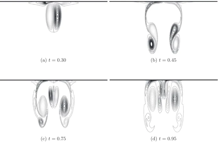
First, we consider a viscous dipole colliding with a rigid, no-slip wall. The collision generates a layer of vorticity near the boundary. This layer rolls up into two monopoles, one either side of the original dipole, which then detach and rebound from the wall along with the original dipole. This collision sequence at Re=1252 is shown in Figure1. This rebound reproduces the well-known results of Kramer, Clercx, and van Heijst.9

As the slip length approaches zero the Navier boundary condition influence matrix reduces to that of the no-slip case. Choosing a sufficiently small slip length in the Navier boundary condition recovers the no-slip dynamics. Numerical experimentation shows thatsL=0.0001 recovers the no-slip dynamics atRe=1252. The comparison between the final time vorticity for a Navier boundary

(a)t= 0.30 (b)t= 0.45

(c)t= 0.75 (d)t= 0.95

0 0.2 0.4 0.6 0.8 1 −1

0 1 2x 10

−4

Time

Es

L

=0

−E

s L

=0.0001

(a) Energy difference

0 0.2 0.4 0.6 0.8 1 0

0.005 0.01 0.015 0.02 0.025 0.03 0.035 0.04

Time

Z s

L

=0

−Z

sL

=0.0001

(b) Enstrophy difference

FIG. 2. Differences for simulated energy and enstrophy of a dipole colliding with a no-slip wall, and a Navier wall withsL =1×10−4as a function of time.

withsL=0.0001 and a no-slip boundary reveals good agreement with small errors in vorticity of order 10−4. The global energy agrees well for the two cases, but the peak enstrophy generation at the wall is greater in the no-slip case. The total energy and enstrophy differences are plotted as a function of time in Figure2.

The most significant difference between the no-slip and Navier boundary cases occurs in the

u-velocity at the boundary, as shown in Figure3. The maximum value of the boundaryu-velocity withsL=0.0001 occurs when the boundary vorticity reaches its maximum, during the collision. The maximum value of the boundaryu-velocity is 0.338, which is comparable to the initialurmsvalue.

0 0.2 0.4 0.6 0.8 1 0

0.05 0.1 0.15 0.2 0.25 0.3

Time

Bo

u

ndary

u

−velocity

(a)t= 0.30 (b)t= 0.45

(c)t= 0.75 (d)t= 0.95

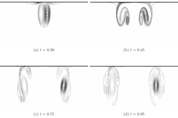
FIG. 4. Sequence of plots showing the simulation of vorticity over the collision with a Navier boundary,sL=0.002,

Re=1252.

2. Intermediate slip length

As the slip length increases, the enstrophy production at the boundary decreases and the gen-erated monopoles weaken. As the impinging dipole approaches the wall the cores separate. The dipole cores separate further and rebound less as slip length decreases. The magnitude of generated vorticity at the wall becomes relatively small compared to that of the impinging dipole, and hence the monopoles formed by roll-up have significantly less effect on the trajectory of the impinging dipole cores. A sequence showing a dipole colliding with a Navier boundary of moderate slip length is shown in Figure4. Notice that the dipole separates more and rebounds less than the dipole colliding with the no-slip wall shown in Figure1.

For longer slip lengths, say greater thansL=0.02, the boundary layer vorticity does not roll up into a distinct monopole, rather filaments of the boundary layer are pulled around the impinging dipole and into the domain. The impinging dipole does not undergo rebound, but the distance from the wall fluctuates. The fluctuation is caused by the filaments of boundary layer vorticity detaching from the wall, and forming small monopoles which wrap around the impinging dipole core, eventually forcing the impinging core away from the wall. The behaviour of the roll-up at the wall for very long slip length,sL=20, and shorter slip length,sL=0.01, is compared in Figure5. Trajectories for a range of slip lengths are shown in Figure6, demonstrating the transition from strong rebounds at short slip lengths to weak, skipping behaviour at longer slip lengths.

The vorticity generated at the wall increases with slip length sL → 0, the global enstrophy production obviously decreases with increasing slip length. The global energy decay increases as

sL→0 as the effect of the boundary becomes stronger. The energy and enstrophy over the period of collision is shown in Figures7and8. For slip lengths shorter than 0.001 the enstrophy difference over the first rebound, fromt=0.2 tot=0.5, is similar, despite the large difference in peak enstrophy. As slip length increases theu-velocity at the wall increases, showing distinct peaks each time the impinging dipole approaches the wall, as seen in Figure9.

3. Slip length sL→ ∞

FIG. 5. Comparison of the boundary vorticity roll-up forsL=20 (left) andsL=0.01 (right) forRe=1252. Only the top left half of the domain is shown. The roll-up is negligible when the slip length is sufficiently large.

and the individual monopoles separate and travel in opposite directions along the wall. This problem can be solved directly without an influence matrix. ChoosingsL = 100 recovers the stress-free dynamics atRe=1252. The trajectories are compared in Figure10for a dipole colliding with a Navier boundary with slip lengthsL =100 and a stress-free wall atRe=1252. Good agreement is observed. The global energy and enstrophy over time is also in good agreement, as shown in Figure 11. Negligible amounts of vorticity are generated at the Navier boundary and at this slip length the stress-free results are recovered.

−0.8 −0.6 −0.4 −0.2 0 −0.1

0 0.1 0.2 0.3 0.4 0.5 0.6 0.7 0.8 0.9

x

y

s

L=0.02

s_L=0.01

s_L=0.004

s_L=0.002

s_L=0.001

s_L=0.0001

0 0.2 0.4 0.6 0.8 1 0.4

0.5 0.6 0.7 0.8 0.9 1

Energy

Time s_L=0.02

s_L=0.01 s

L=0.004

s_L=0.002

s_L=0.001

s_L=0.0001

FIG. 7. Energy as a function of varying slip lengthsL.

B. Comparison of the penalisation method with the influence matrix method

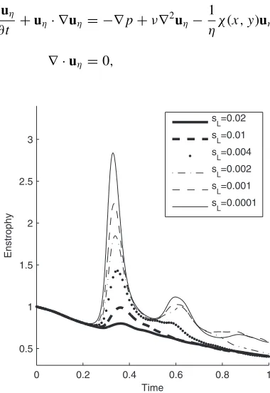
Volume penalisation avoids the use of body-fitted unconstructed meshes by penalising the velocity on the surface of an object surrounded by fluid. This allows the use of fast spectral methods on Cartesian grids to solve the incompressible Navier-Stokes equations in bounded domains. The penalisation method aims to solve the Navier-Stokes equation in a channel domain by solving a similar problem on a doubly-periodic domain and forcing the velocity to be small between the channel wall and they-periodic boundaries. We do this by solving

∂u_η

∂t +uη· ∇uη = −∇p+ν∇ 2_u

η−_η1χ(x,y)uη,

(42)

∇ ·uη =0,

0 0.2 0.4 0.6 0.8 1 0.5

1 1.5 2 2.5 3

Enstrophy

Time

s_L=0.02

s_L=0.01 s

L=0.004

s_L=0.002

s_L=0.001

s_L=0.0001

0 0.2 0.4 0.6 0.8 1 0

1 2 3 4 5 6 7 8 9

Wall

u

−velocity

Time

s_L=0.02 s

L=0.01

s_L=0.004

s_L=0.002

s_L=0.001

s_L=0.0001

FIG. 9. Simulatedu-velocity at the wall for varying slip length over the collision time atRe=1252.

whereu_ηis the penalised velocity,χis the penalisation function, which is zero in the fluid domain and takes the value one between the channel wall and the periodicy-boundaries, andηis the penalisation parameter. It can be shown that the solution of problem(42)converges slowly to the solution of the full Navier-Stokes problem in the channel domain asη→0.6

By plotting the tangential velocity as a function of strain rate at the channel wall location, Nguyen van yen, Farge, and Schneider1 show that the penalisation method can be used to approximate no-slip boundary conditions. More specifically, they demonstrate that their results are close to those for a Navier boundary condition with slip lengthsLapproximately equal to 4/Re. AtRe=1252, for example, this givessL≈0.003. From our previous discussion, we expect this to give good agreement

−0.5 −0.4 −0.3 −0.2 −0.1 0 −0.1

0 0.1 0.2 0.3 0.4 0.5 0.6 0.7 0.8 0.9

x

y

s

L=100

Stressfree

0 0.1 0.2 0.3 0.4 0.5 −2.5

−2 −1.5 −1 −0.5 0

x 10−3

EsL=100

−E

Stressfree

Time

(a) Energy difference

0 0.1 0.2 0.3 0.4 0.5 −2.5

−2 −1.5 −1 −0.5 0

x 10−3

Time

ZsL=100

−Z

Stressfree

(b) Enstrophy difference

0 0.1 0.2 0.3 0.4 0.5 −0.05

0

Time

u

(0)

sL=100

−

u

(0)

Stressfree

(c) Wallu−velocity difference

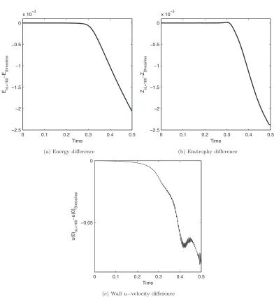
FIG. 11. Difference between energy, enstrophy, andu-velocity at the collisional wall vs. time, for a dipole colliding with a Navier boundary,sL=100 and a stress-free boundary atRe=1252. The oscillations in boundaryu-velocity are due to the generation of weak velocity filaments in the case with the Navier boundary condition.

with no-slip trajectories over the initial rebound, but to diverge at later times. As the Reynolds number decreases, thesL=4/Reapproximation becomes less accurate, but the penalisation method still approximates a Navier boundary, with a slip length which may be determined in the usual way. In their paper, Nguyen van yen, Farge, and Schneider1 use a smoothχ penalisation function. We choose instead to use a Heaviside penalisation function. This gives a precise boundary location, avoiding difficulties in choosing the boundary location. The use of a Heaviside function, however, introduces Gibbs oscillations in the solution near to the step. Keetels et al.13 _{showed that these}

oscillations do not affect the stability of the calculation, nor the overall result. Any ringing in the solution can therefore be removed by using a post-processing filter. There exist many techniques to remove ringing from data. Keetels et al.13 _{used a spectral mollification procedure due to Tadmor}

and Tanner.14 _{We chose to use a simple weighted averaging filter. Any minor errors introduced by}

0.95 0.96 0.97 0.98 0.99 1 −0.05

0 0.05 0.1 0.15 0.2 0.25 0.3 0.35 0.4 0.45

Cross−section at x=−0.67

Relative difference in vorticity

N_x=N_y=1024, η=1×10−4

N_x=N_y=1024, η=5×10−4

N

x=Ny=2048, η=1×10 −6

N_x=N_y=4096, η=5×10−5

FIG. 12. The difference between the vorticity calculated by the penalisation method and the vorticity calculated by the influence matrix methodNx=512,Ny=768 with no-slip boundary conditions as the dipole rebounds from the wall.

Subsequently, Nguyen van yen15 proved that the penalisation method using a Fourier pseu-dospectral method is effectively first order inN−1, due to the jump at the boundary. We compare relative differences in vorticity for representative cross-sections from the penalty method as discussed above and the influence matrix method with no-slip boundary conditions. TheO(N−1_{) convergence}

of the penalisation method to the solution calculated by the influence matrix method is shown in Figure12. Results are shown forRe=626, timet=0.4, during the dipole collision with the wall, for increasing numbers of mesh points. Convergence with the penalisation parameterη → 0 is very slow as expected. At low resolution the magnitude of the boundary vorticity is significantly underestimated. This leads to a weaker rebound, and hence a phase error in vorticity far from the wall. As the resolution increases, the boundary vorticity estimate improves and consequently the vorticity inside the domain is more accurately estimated.

C. Energy dissipation rate comparison

Nguyen van yen, Farge, and Schneider1investigated the phenomenon of anomalous dissipation. They found energy dissipating structures which persisted in the vanishing viscosity limit.

There are two regimes occurring in the collision simulation. In the first regime, the dipole is far from the wall and the effects of the boundary are negligible and the energy dissipation scales like

E(t2)−E(t1)∝ Re−1. (43)

In the second regime, the dipole is close to the wall. Prandtl16resolved d’Alambert’s paradox for flows where the effects of viscosity occur only in a boundary layer of thickness of orderRe−1/2. Prandtl16showed that in the boundary layer the energy dissipation scales like

E(t2)−E(t1)∝ Re−1/2. (44)

The total energyE(t) satisfies

d E

dt +2νZ =0, (45)

whereZ is the global enstrophy. Thus, the energy dissipation rate is directly proportional to the enstrophy growth. Nguyen van yen, Farge, and Schneider1_{found thatZ∝Reand hence an energy}

TABLE I. Table of parameters used in the calculations.

Re Nx Ny ν×10−4 δt×10−6 4/Re

870 512 768 7.2 4.8 0.005

1160 512 768 5.4 4.8 0.003

1740 512 768 3.6 4.8 0.002

2610 1024 2048 2.7 4.8 0.0015

3480 1024 2048 1.8 4.8 0.001

5580 2048 4096 1.15 2.0 0.0007

6962 2048 4096 0.9 2.0 0.0006

Keetelset al.17_{used an oscillating plate model to predict the vorticity, enstrophy, and}

palinstro-phy production from a dipole colliding with a no-slip boundary. In particular, they find a scaling of

Z∝Re0.75 _{for Reynolds number less than some critical value, andZ∝Re}0.5_{for Reynolds number}

greater than the critical value. The critical Reynolds number was found to be aroundRe=20 000, higher than considered here and higher than considered by Nguyen van yen, Farge, and Schneider.1 The predicted scaling agrees well with observed peak enstrophy in their simulations. Importantly these results suggest that the enstrophy growth, and hence energy dissipation, will slow as the Reynolds number becomes increasingly large.

We compare the total energy dissipation and enstrophy growth, as a function of Reynolds number, over one rebound for the no-slip boundary condition, the Navier boundary condition with fixed slip lengths,sL=0.003 andsL=0.0001, and a Navier boundary condition withsL=4/Re. The choice of slip length has a non-zero but negligible effect on the Reynolds number. The slip length relationsL=4/Reis motivated by the finding of Nguyen van yen, Farge, and Schneider1for the boundary condition of the penalisation method and similarlysL=0.003 is the slip length given by this approximation forRe≈1300, near the lower Reynolds numbers considered in Nguyen van yen, Farge, and Schneider.1_{As discussed earlier, the slip lengths}

L=0.0001 should approximate the no-slip results. The parameters chosen in the calculations are shown in TableI.

D. Energy dissipation far from the wall

It is easy to identify the first regime, where the dipole is far from the wall. The time interval chosen was t=0 tot=0.2, for each boundary condition case the dipole was still intact, and far from the wall. The energy dissipation scaling(43)was found to hold satisfactorily for all boundary condition cases considered, as shown in Figure13.

700 2000 5000 10000 0.01

0.02 0.05 0.1

Re

E(0.2)-E(0)

Re-1

E. Energy dissipation and energy dissipation rate near the wall

From Nguyen van yen, Farge, and Schneider1_{we expect any energy dissipating structures to}

occur in the boundary layer. It is therefore critical to choose a time interval that captures the behaviour of these structures. If the time interval is too short it will not show the energy dissipating structures, if the time interval is too long, the boundary layer will separate and move into the domain, violating Prandtl’s theory. If the time interval is misplaced, it is possible to observe energy growth. To identify the collision, we follow Nguyen van yen, Farge, and Schneider1_{and choose the time interval where}

the energy scaling best satisfies Prandtl’s energy dissipation result, where energy dissipation scales likeRe−0.5_{. To do this we first estimate the time of the collision by studying the vorticity plots. We}

then search for time intervals near our estimate where Prandtl’s result is valid. For each time interval, the energy dissipation as a function of Reynolds number is calculated, and a least squares regression line is fitted to the logarithm of the data. The slope of this line should be−1/2. We also obtain a 95% confidence interval on the least squares fit in the standard way. The time interval which gives the slope closest to −1/2 is declared to be the interval over which the collision occurs. This time interval varies between the three cases considered.

First we consider thesL=0.003 case. The energy dissipation as a function of Reynolds number is shown in Figure14for a range of collision time intervals. The best collision time interval ist1=

0.27 tot2=0.49, which gives the energy decayE(t2)−E(t1)∝Re−α, whereα= −0.53±0.05. The

corresponding enstrophy growth starts to saturate to a constant at higher Reynolds numbers. Since enstrophy growth is slower than linear with Reynolds number, from(45)the energy dissipation rate is proportional to some power of viscosity, and this will vanish in the limitν→0.

The energy difference results are similar for the no-slip,sL =0.0001, andsL=4/Recases. This is reasonable, since all cases approximate the true no-slip boundary conditions. It is, however, difficult to satisfy Prandtl’s result in these cases, while finding enstrophy growth in the same time interval. The best slope that is achieved is−0.43 over time intervalst1=0.2 tot2=0.49, as shown in

Figure15. This is in fact the longest time interval possible, as it starts at the end of the wall-free regime. The crucial difference between these three cases occurs in the enstrophy growth results, in particular the rate at which enstrophy growth varies with Reynolds number. The no-slip,sL=0.0001, andsL=4/Recases, are shown in Figure16. The no-slip andsL=0.0001 cases start saturating in a manner similar to thesL=0.003 case. The enstrophy growth as a function of Reynolds number, for

600 1000 2000 5000 9000 0.05

0.07 0.1 0.15 0.25

Reynolds number

E(t

2

)−E(t

1

)

E(0.49)−E(0.24) E(0.49)−E(0.25) E(0.49)−E(0.26) E(0.49)−E(0.27)

Re−1/2

(a) Energy dissipation

500 1000 2000 5000 9000 10−2

10−1 100

Z(t

2

)−Z(t

1

)

Reynolds number Z(0.49)−Z(0.25)

Z(0.49)−Z(0.26) Z(0.49)−Z(0.24) Z(0.49)−Z(0.27)

Re1

(b) Enstrophy growth

600 1000 2000 5000 9000 0.09

0.1 0.15 0.25

Reynolds number

E(t

2

)−E(t

1

)

E(0.48)−E(0.2) E(0.49)−E(0.2)

E(0.48)−E(0.21) E(0.49)−E(0.21)

Re−1/2

(a) No-slip

600 1000 2000 5000 9000 0.09

0.15 0.25

Reynolds number

E(t

2

)−E(t

1

)

E(0.48)−E(0.2) E(0.49)−E(0.2)

E(0.49)−E(0.2) E(0.48)−E(0.21)

Re−1/2

(b)sL= 0.0001

600 1000 2000 5000 9000 0.07

0.1 0.15 0.25

Reynolds number

E(t

2

)−E(t

1

)

E(0.47)−E(0.2) E(0.49)−E(0.2)

E(0.47)−E(0.21) E(0.49)−E(0.21)

Re−1/2

(c)sL= 4/Re

FIG. 15. Energy dissipation as a function of Reynolds number near the wall with boundary conditions as shown. For all the boundary conditions the best agreement with Prandtl’s scaling isRe−0.43_{, and the best collision time interval ist}

1=0.20 to

t2=0.49.

the best time intervals for the no-slip,sL=0.0001,sL=0.003, andsL=4/Recases are compared in Figure 17, clearly showing the difference in slope between the no-slip,sL =0.0001, andsL = 0.003, compared to thesL=4/Recase. In the no-slip,sL=0.0001, andsL=0.003 cases, enstrophy grows more slowly than linearly with Reynolds number and there will be no energy dissipation in the vanishing viscosity limit. For thesL=4/Recase, the enstrophy difference results are approximately linear with Reynolds number, consistent with the findings of Nguyen van yen, Farge, and Schneider.1

For lower Reynolds numbers the enstrophy growth is much more rapid, and we have omitted

Re<1700 from Figure17for clarity.

1. Energy dissipation comparison with the penalty method

500 1000 2000 5000 9000 10−1

100

Z(0.48)−Z(0.2)

Z(t

2

)−Z(t

1

)

Reynolds number Z(0.49)−Z(0.2)

Z(0.48)−Z(0.21)

Z(0.49)−Z(0.21) Re1

(a) No-slip

500 1000 2000 5000 9000 10−1

100

Z(0.48)−Z(0.2)

Z(t

2

)−Z(t

1

)

Reynolds number Z(0.49)−Z(0.2)

Z(0.48)−Z(0.21)

Z(0.49)−Z(0.21) Re1

(b)sL= 0.0001

500 1000 2000 5000 9000 10−2

10−1 100

Z(t

2

)−Z(t

1

)

Reynolds number Z(0.47)−Z(0.2)

Z(0.49)−Z(0.2) Z(0.47)−Z(0.21)

Z(0.49)−Z(0.21) Re1

(c)sL= 4/Re

FIG. 16. Enstrophy difference results for the no-slip,sL=0.0001, andsL=4/Reboundary cases. The best collision time interval ist1=0.20 tot2=0.49.

penalisation method converges approximately linearly withNy, and that furthermore the slip length is approximately inversely proportional toNyand hence constant for constantNy. The slip length for the step penalisation function was found to besL=0.002 forNx=Ny=1024, andsL=0.0004 for

Nx=Ny=2048, while for the smooth penalisation functionsL=0.008 forNx=Ny=1024, andsL

=0.003,Nx=Ny=2048. Note that we only expect the penalisation method withsL=0.0004 for

Nx=Ny=2048 to approximate the no-slip boundary condition. In Figure18the enstrophy growth rates for the penalisation method withNx=Ny=1024 andNx=Ny=2048 for both choices ofχ are compared to the results (repeated from Figure17) for the no-slip boundary condition, using the influence matrix method.

2000 3000 5000 9000 0.1

0.25 0.5 1 1.5

Re

Z(t

2

)-Z(t

1

)

s_L=0.0001 s

L=0.003

s_L=4/Re

No-slip Re1

FIG. 17. Enstrophy difference results for the no-slip,sL=0.003,sL=0.0001, andsL=4/Reboundary condition cases, taking the best collision time interval for all cases. For no-slip,sL=0.003,sL=0.0001, andsL=4/Rethe best time interval ist1=0.20 tot2=0.49. For thesL=0.003 the best time interval ist1=0.27 tot2=0.49.

1700 3000 5000 8000 0.3

0.7 1.8

Reynolds number

Z(t

2

)−Z(t

1

)

Re1 No−slip Step N_x=N_y=2048 Smooth N_x=N_y=2048 Step, N_x=N_y=1024

Smooth, N_x=N_y=1024

smooth penalisation function results in a significantly larger slip length and hence smaller enstrophy growth than the step function treatment.

IV. CONCLUSIONS

A normal incidence dipole wall collision is a notoriously difficult problem, due to the rapid generation of vorticity at the boundary, which makes it a suitable benchmarking test for numerical methods solving the streamfunction-vorticity problem. We have studied the range of behaviours between the two extreme cases of a dipole colliding with a stress-free boundary and a dipole colliding with a no-slip boundary. For small slip length the trajectory of the dipole after collision approximates the trajectory of a dipole which has collided with a no-slip wall, but the enstrophy generated at the wall is significantly lower, and hence the trajectories of the dipoles will diverge at later times. The growth in global enstrophy over the collision time decreases with increasing slip length, and increases withRe, for moderate Reynolds numbers. At the highest Reynolds numbers considered the enstrophy growth starts decreasing with increasingRe. Therefore, if Reynolds number is increased and slip length is decreased simultaneously, the overall trend in enstrophy growth will be steeper than if the slip length is held constant.

The result of Nguyen van yen, Farge, and Schneider1_{is that enstrophy growth over the collision}

time grows linearly with Reynolds number, so implying that the energy dissipation tends to a constant as viscosity vanishes. This is a consequence of the slip lengthsL∝Re−1, which follows if linearly increasing resolution is used (to properly resolve detail) with increasing Reynolds number, because of the approximate linear dependence ofsLonNy. Repeating the numerical experiments of Nguyen van yen, Farge, and Schneider1with the fully resolved influence matrix method showed sublinear enstrophy growth in the vanishing viscosity limit for anyfixedslip length.

For the dipole-wall collision, the penalisation method requires very high resolution to ac-curately estimate the magnitude of the vorticity generated at the boundary. Both high resolution and a step function boundary treatment are required to ensure the small slip length that gives a good approximation to the no-slip case. Furthermore, fixed resolution, withNx,Ny=constant is required to keep the slip length fixed as Reynolds number is varied, which is necessary in or-der to obtain consistent energy dissipation results in the vanishing viscosity limit. This simple restriction on resolution avoids difficulties of interpretation caused by the approximate boundary conditions.

Extensions of the present work will consider the true nature of the boundary condition in the volume penalisation method, non-normal incidence collisions which may be benchmarked against Clercx and Bruneau,18and extending the compact finite difference method to circular domains.

1_{R. Nguyen van yen, M. Farge, and K. Schneider, “Energy dissipating structures produced by walls in two-dimensional}

flows at vanishing viscosity,”Phys. Rev. Lett.106, 184502 (2011).

2_{P. Orlandi, “Vortex dipole rebound from a wall,”Phys. Fluids A2, 1429 (1990).}

3_{H. J. H. Clercx and G.-J. F. van Heijst, “Dissipation of kinetic energy in two-dimensional bounded flows,”Phys. Rev. E} 65, 066305 (2002).

4_{W. Kramer, “Dispersion of tracers in two-dimensional bounded turbulence,” Ph.D. thesis (Eindhoven University of}

Tech-nology, Eindhoven, Netherlands, 2007).

5_{B. Kadoch, D. Kolomenskiy, P. Angot, and K. Schneider, “A volume penalization method for incompressible flows and}

scalar advection-diffusion with moving obstacles,”J. Comput. Phys.231, 4365–4383 (2012).

6_{P. Angot, C.-H. Bruneau, and P. Fabrie, “A penalization method to take into account obstacles in incompressible viscous}

flows,”Numer. Math.81, 497–520 (1999).

7_{Y. Stokes and G. Carey, “On generalised penalty approaches for slip, free surface, and related boundary conditions in}

viscous flow simulation,”Int. J. Numer. Methods Heat Fluid Flow21, 668–702 (2011).

8_{O. Daube, “Resolution of the 2D Navier-Stokes equations in velocity-vorticity form by means of an influence matrix}

technique,”J. Comput. Phys.103, 402–414 (1992).

9_{W. Kramer, H. J. H. Clercx, and G.-J. F. van Heijst, “Vorticity dynamics of a dipole colliding with a no-slip wall,”Phys.}

Fluids19, 126603 (2007).

10_{A. Stephan, personal communication (2012).}

11_{S. K. Lele, “Compact finite difference schemes with spectral-like resolution,”J. Comput. Phys.103, 16–42 (1992).} 12_{H. J. H. Clercx, S. R. Maassen, and G.-J. F. van Heijst, “Decaying two-dimensional turbulence in square containers with}

13_{G. H. Keetels, U. D’Ortona, W. Kramer, H. J. H. Clercx, K. Schneider, and G.-J. F. van Heijst, “Fourier spectral and}

wavelet solvers for the incompressible Navier–Stokes equations with volume-penalization: Convergence of a dipole–wall collision,”J. Comput. Phys.227, 919–945 (2007).

14_{E. Tadmor and J. Tanner, “Adaptive filters for piecewise smooth spectral data,”IMA J. Numer. Anal.25, 635–647 (2005).} 15_{R. Nguyen van yen, D. Kolomenskiy, and K. Schneider, personal communication (2012).}

16_{L. Prandtl, inProceedings of the 3rd International Congress of Mathematicians, Heidelberg, 1904, edited by A. Krazer} (Taubner, Leipzig, 1905), p. 484.

17_{G. H. Keetels, W. Kramer, H. J. H. Clercx, and G. F. van Heijst, “On the Reynolds number scaling of vorticity production}

at no-slip walls during vortex-wall collisions,”Theor. Comput. Fluid Dyn.25, 293–300 (2011).