Efficient abstracting of dive profiles using a broken-stick model
1Short running title: Efficient abstracting of dive profiles 2
3
Theoni Photopoulou (corresponding author) 4
Centre for Statistics in Ecology, Environment and Conservation, Department of 5
Statistical Sciences, University of Cape Town, Rondebosch 7701, Cape Town, South 6
Africa 7
Email: [email protected] 8
Philip Lovell 9
Sea Mammal Research Unit, Scottish Oceans Institute, University of St Andrews, 10
Scotland KY16 8LB, UK 11
Michael A Fedak 12
Sea Mammal Research Unit, Scottish Oceans Institute, University of St Andrews, 13
Scotland KY16 8LB, UK 14
Len Thomas 15
Centre for Research into Ecological and Environmental Modelling, The Observatory, 16
University of St Andrews, Scotland KY16 9LZ, UK 17
Jason Matthiopoulos 18
Institute of Biodiversity, Animal Health and Comparative Medicine, Graham Kerr 19
Building University of Glasgow, Glasgow, Scotland G12 8QQ, UK 20
Summary 26
1. For diving animals, animal-borne sensors are used to collect time-depth 27
information for studying behaviour, ranging patterns and foraging ecology. Often, this 28
information needs to be compressed for purposes of storage or transmission. Widely 29
used devices called Conductivity-Temperature-Depth Satellite Relay Data Loggers 30
(CTD-SRDLs) sample time and depth at high resolution during a dive and then 31
abstract the time-depth trajectory using a broken-stick model (BSM). This 32
approximation method can summarise efficiently the curvilinear shape of a dive, 33
using a piecewise linear shape with a small, fixed number of vertices. 34
2. We present the process of abstracting dives using the BSM and quantify its 35
performance, by measuring the uncertainty associated with the profiles it produces. 36
We develop a method for obtaining a confidence zone and an index for the 37
goodness-of-fit (dive zone index, DZI) for abstracted dive profiles. We validate our 38
results with a case study using dives from elephant seals (Mirounga spp.). We use 39
Generalised Additive Models (GAMs) to determine if the DZI can be used as a proxy 40
for an absolute measure of fit, and investigate the relationship between the DZI and 41
dive shape. 42
3. We found a strong correlation between the residual sum of squares (RSS) for the 43
difference between the detailed and abstracted profiles and the DZI and maximum 44
residual (R4), for dives resulting from CTD-SRDLs (69% deviance explained). On it’s 45
own the DZI explained a lower percentage of deviance which was variable for 46
abstracted dives with different numbers of points. We also found evidence for 47
systematic differences in the DZI for different dive shapes (65% deviance explained). 48
4. Although the proportional loss of information in the abstraction of time-depth dive 49
abstracted profile by reversing the abstraction process. Our results suggest that 51
together the DZI and R4 can be used as a proxy for the RSS, and we present the 52
method for obtaining these metrics for BSM-abstracted profiles. 53
54
Keywords: animal telemetry, broken-stick model, CTD-SRDL, dive profile, dive type, 55
dive zone index, elephant seal, data abstraction 56
INTRODUCTION
76Data abstraction in animal telemetry: needs and consequences 77
One of the most effective ways to remotely study movement and behaviour in marine 78
animals is to use animal-borne sensors. Satellite-linked and archival animal 79
telemetry devices have developed rapidly, driven by questions about the behaviour 80
and movement of large vertebrates at sea. A range of purpose-built hardware and 81
software is widely available for deployment on animals. Although animal telemetry 82
devices are able to record information at high temporal and spatial resolution, in 83
many cases devices cannot be recovered, which means the data have to be 84
transmitted. Additionally, it is seldom possible to transmit all data that are collected 85
during a deployment, because the quantity and resolution of the received telemetry 86
data are constrained by several factors: the desired observation time, battery life of 87
the device, bandwidth of the communication system used to relay data, behaviour of 88
the animal, and the software specifications. This means that not all information that 89
is recorded can be recovered. Consequently, data abstraction (defined here as 90
reduction in volume to a simplified representation of the original) is unavoidable for 91
many types of telemetry device. 92
93
The trade-off between temporal data resolution (i.e., the rate of data sampling and 94
delivery) and the operational longevity of the telemetry device has driven the 95
development of efficient software and memory-saving processing algorithms. One of 96
these is a broken-stick model (BSM), used for the abstraction of two-dimensional 97
dive trajectories (time-depth dive profiles) on-board telemetry devices prior to 98
transmission (Fedak et al. 2002). BSMs are change-point models, falling under 99
time-series. The piecewise linear profile of a time-series, generated by an efficient 101
linear abstraction method, should have low average deviation from the detailed dive 102
profile. When processing takes place on a small device with limited power for 103
processing and transmissions, it is advantageous to represent piecewise linear 104
profiles using a fixed and small number of bits of information, particularly when using 105
CLS Argos, where message size is fixed (Argos 2011). The algorithm should also be 106
time-efficient, scale linearly in execution time with dive duration, and consistently 107
encode biologically relevant information that might enable inferences on dive 108
function. The BSM fulfils these criteria and was adopted as the default dive 109
abstraction algorithm on CTD-SRDLs in 2006 (pers. comm. Phil Lovell). The 110
predecessor of this model placed breakpoints at locations of maximum inflection in 111
the detailed profile, and while it performed equally well, processing required more 112
time and energy (Fedak, Lovell & Grant 2001). The BSM was chosen empirically, 113
because it was found to provide a highly satisfactory compromise between the 114
priorities described above. However, its performance has not been formally tested, 115
nor have the consequences of its performance on the biological and ecological 116
conclusions that are drawn in studies using dive profiles abstracted with the BSM. 117
118
In ecology, change-point models have a long history (MacArthur 1957; MacArthur & 119
MacArthur 1961) and have seen application in a range of fields, e.g., in 120
oceanography to reduce data volume (Rual 1989), to identify edge effects in plant 121
communities (Toms & Lesperance 2003), to locate ontogenetic shifts in southern 122
elephant seal diet using stable isotopes (Authier et al. 2012) and in a Bayesian 123
context applied to allometric relationships between tree height and diameter 124
time-depth dive profile as an example (Figure 1). We call abstracted those dive 126
profiles that have been processed and reduced in resolution using this algorithm. We 127
call detailed those dive profiles that are recorded at regular and frequent time 128
intervals, at the sampling resolution of the device. 129
130
Assessing uncertainty in abstracted dive profiles from elephant seals 131
(Mirounga sp.) as a case study 132
The need for abstraction becomes critical for deployments on wide-ranging marine 133
species, such as seals and turtles, when geographic and temporal data coverage is 134
of interest, and when devices cannot be recovered. For elephant seals and other 135
phocid seals for example, complete time-series of year-round locations and 136
behaviour may be more biologically interesting than detailed information over short 137
periods, and more useful for understanding their life-histories (McConnell, Chambers 138
& Fedak 1992; Hebblewhite & Haydon 2010). Until now, the uncertainty associated 139
with abstracted profiles has not been quantified and the implications for ecological 140
studies that use abstracted profiles have not been assessed. 141
142
Abstracted profiles are, by construction, information-poor versions of the detailed 143
trajectories, but since the abstraction process is known in the case of CTD-SRDLs, it 144
is possible to reverse the deterministic steps and retrieve some of the information. 145
Historically, once the abstraction was completed, the high-resolution time-depth 146
profile was overwritten, but current tags store all information that they record, and 147
this can be accessed if the tag is retrieved. Here, we show that it is possible to 148
construct a 100% confidence zone around an abstracted profile (i.e., upper and 149
compare the zone for different dives. This confidence zone is hereafter referred to as 151
the dive zone, and the relative measure of maximum deviation of the abstracted 152
profile, from the detailed profile, is referred to as the dive zone index (DZI). 153
154
The consequences of the abstraction regime by BSM are investigated here using 155
detailed and abstracted dive profiles, from northern (M. angustirostris) and southern 156
elephant seals (M. leonina), as a case study. Elephant seals are large-bodied, long-157
lived and abundant marine mammals. They spend many months at sea in the open 158
ocean and in coastal or marginal ice zones (McConnell et al. 1992; Jonker & Bester 159
1998; Campagna et al. 2007; Bailleul et al. 2007; Biuw et al. 2010). They frequently 160
visit high latitudes for extended periods, diving deeply and almost continually, 161
returning to land twice a year to breed and moult. CTD-SRDLs are regularly used in 162
studies of their movement and diving behaviour, and that of other wide-ranging 163
phocid seals. 164
165
The characterisation of dives into types, based on dive parameters, has been a 166
popular approach to the study of diving behaviour (Hindell, Slip & Burton 1991; 167
Schreer & Testa 1996; Schreer, Kovacs & O’Hara Hines 2001; Baechler 2002). In 168
general, the identification of types or groups of behaviour is useful for comparing 169
behavioural patterns and activity budgets between individuals and in different spatial 170
and temporal contexts, and is carried out using a wide range of methods including 171
empirical methods, machine learning, and state-space methods, to name a few (e.g., 172
Fauchald & Tveraa 2003; Thums, Bradshaw & Hindell 2008; McKellar et al. 2014). 173
BSM dives are used widely in studies of diving behaviour and physiology (e.g., 174
considering or accounting for uncertainty in the abstracted dive profiles. Ignoring the 176
uncertainty in BSM-derived time-depth profiles may lead to incorrect inferences if the 177
BSM output has substantial error associated with it, and if dives with different shape 178
characteristics differ systematically in the amount of error associated with them. This 179
computationally expedient method has been thought to perform well at capturing 180
biologically relevant aspects of time-depth dive profiles, but this impression has, to 181
date, remained anecdotal. 182
183
Aims and questions 184
In this paper we aim to explain the BSM for dive profile abstraction, provide a 185
method that extracts as much information as possible from abstracted dive data, and 186
improve the interpretability of abstracted dive profiles. To do this we 1) present an 187
overview of the process by which the BSM generates abstracted dive profiles; 2) 188
assess the performance of the BSM for dive profile representation, by comparing 189
detailed and abstracted time-depth dive profiles from elephant seals, as a case 190
study; 3) present a three-step method for obtaining, post hoc, the depth limits on the 191
detailed dive (i.e., the dive zone) based on its BSM abstracted profile; 4) develop an 192
index of goodness-of-fit of abstracted dives (i.e., DZI) and use detailed dive profiles 193
to validate it; and 5) use this index to determine if there are systematic differences in 194
the amount of error associated with different dive types, following (Hindell et al. 195
1991). 196
197
We recast these five aims as research questions: 1) How does the BSM work for 198
dive profile abstraction? How does the representation of the detailed dive change 199
3) What can we learn from abstracted dives? 4) How is the DZI derived? And, 5) Can 201
the DZI be used as a proxy for the RSS? Does the DZI vary systematically between 202
dive types? 203
204
MATERIALS AND METHODS
205How does the BSM work for dive profile abstraction? 206
The BSM is an iterative process. For time-depth dive profiles, it is based on 207
minimising the vertical distance (i.e., difference in depth) between the detailed 208
trajectory recorded by the tag and the abstracted dive profile being proposed, at the 209
sampling resolution of the dive (for CTD-SRDLs 4s, 8s, 16s or 32s). We call these 210
vertical distances residuals (Figure 1). The basic principle of the model is that at 211
each iteration, the residuals are calculated, and the point with the biggest residual is 212
added to the abstracted profile. At the first iteration, which we call step zero, the 213
abstracted profile consists only of the start and end points of the dive, forming a 214
straight line at what the tag perceives to be zero depth. This corresponds to a depth 215
buffer at the surface (0-6 m), which is intended to exclude any less interesting 216
shallow undulations from the dive record, that would compete with regular deep 217
dives for transmission. The distance from this straight line to the detailed profile is 218
measured at each time point and the point at which the piecewise linear abstracted 219
profile deviates most from the detailed profile is added to the abstracted profile, 220
creating two new line segments. This is called a breakpoint. This step creates a new 221
piecewise linear profile comprising I+2 points, connected by linear segments, and 222
completes one iteration of the model (Figure 1). 223
224
the point with the greatest departure is selected as the next breakpoint and added to 226
the profile. This process is repeated until the desired number of breakpoints is 227
reached, and the resulting piecewise linear abstracted profile has been constructed. 228
When the abstraction process is complete, the abstracted time-depth dive profile 229
includes I+2time points (T1 to TI), and the corresponding I depth points (D1to DI). 230
The first and last points, (T0,TI+1, D0 and DI+1) are not transmitted. At T0 time is 231
considered to be zero and at TI+1 the time elapsed since the beginning of the dive 232
will equal the dive duration. Similarly, at D0 and Di+1, the depth will both be 0-6 m. 233
The order in which the time-depth points were selected is not stored or transmitted. 234
235
How does the representation of the detailed dive change with increasing BSM 236
points? 237
Using detailed dives from four high-resolution datasets, each representing a 238
continuous dive record from one individual (10943, 12454, 12453 and 12451 in 239
Table 1), we estimated the proportion of high-resolution samples that was 240
represented by the number of BSM points in the corresponding abstracted dive 241
profile (Table 2). We generated an abstracted profile with 3-12 BSM points for each 242
study dive. This resulted in a dataset of 2400 proportions, from 240 dives. 243
244
Is the sample of study dives representative? 245
Four iterations of the BSM are carried out on-board CTD-SRDLs, resulting in a dive 246
profile consisting of six time-depth points: two at the surface, and four at depth, at 247
irregular times, which vary from dive to dive. The number of iterations of the BSM 248
algorithm to be carried out on CTD-SRDLs was chosen as the minimum sufficient 249
of computations low (Fedak et al. 2001). 251
252
We confirmed that the sample of detailed dives from the four individuals was 253
consistent with elephant seal diving behaviour in general. To do this, the DZI was 254
calculated for a sample of 4,000 abstracted dives from 45 southern elephant seals 255
instrumented in four different field seasons (1,000 dives each from two post-moult 256
deployments and two post-breeding deployments; ct40, ct45, ct49, ct58) over two 257
years at the island of South Georgia, South Atlantic (Table 1). The resulting 258
distribution of DZI was visually compared with the distribution of DZI for the detailed 259
dives (Appendix S2, Figures S2.1 and S2.2). 260
261
What can we learn from abstracted dives? 262
The process by which abstracted dive profiles arise when they are collected by CTD-263
SRDL, is known, therefore it is possible to reverse the deterministic steps and obtain 264
limits to the depth at which the trajectory could have passed, before it was 265
abstracted. The information required to build the dive zone (the 100% confidence 266
zone for depth) includes the 1) temporal resolution at which the dive was recorded 267
by the tag, the I+2 locations, in time and depth (including maximum dive depth), 2) 268
the residual associated with the final, I+1th breakpoint, and critically, 3) the order in 269
which breakpoints were selected during abstraction. The temporal resolution of the 270
detailed dive data is known from the duration of the dive, and the locations are 271
received in the satellite transmissions, but the residuals and the order in which the 272
breakpoints were added need to be determined. Constructing the dive zone involves 273
three steps. 274
First, to find the order in which points were added to the profile, the BSM must be 276
applied to the already abstracted dive trajectory (Figure 2). At each of the I iterations, 277
one of the breakpoints is selected as the point of greatest deviation hence retrieving 278
the order in which the breakpoints were added. 279
280
Second, to determine the limits of the zone, the residuals corresponding to the 281
breakpoints need to be calculated. It is tempting to assume that the residual 282
associated with the Ith breakpoint, RI, applies to all segments in the final profile, 283
determining the limits of the dive zone. This is not the case. The limits of the dive 284
zone at each iteration of the model interact with those from previous iterations. As 285
breakpoints are added to the profile, the dive zone changes shape and size. 286
Although the dive zone will always get smaller with subsequent iterations of the 287
algorithm, this geometric effect means that the dive zone needs to be constructed 288
based on all iterations of the model, up to the last one. Furthermore, the resulting 289
dive zone at the final iteration is not symmetric around any segments in a profile and 290
all breakpoints touch the limit of the dive zone (Figure 3). 291
292
The depth points selected by the BSM are coded before transmission according to a 293
pseudo-logarithmic mantissa and exponent representation. With this representation, 294
resolution can be made proportional to the scale of the number being represented, 295
making it useful for depth. Data are then truncated during the decoding process, 296
once they are received. As a consequence, the received depth measurements are 297
binned (i.e. each reported depth has an upper and lower bound) and bin width 298
increases with depth. Bin width is usually smaller than the dive zone height at each 299
dive where the depths along the line segment near the bottom of the dive exceed the 301
known accuracy of the greatest depth reached during the dive. This is justified since 302
we know that no point in the true profile can be deeper than the maximum depth 303
recorded by the tag. Depth is also truncated at each breakpoint, for the same 304
reason, so the dive zone appears “pinched” at each breakpoint (Figure 3). 305
306
When the Ith iteration is complete, it is known with certainty that there were no points 307
in the detailed trajectory that had a greater residual than the one corresponding to 308
the last point (Figure 2). All other depth points in the true trajectory will now have a 309
smaller vertical distance to the abstracted profile. 310
311
Third, to construct the dive zone, a number of equally spaced time points need to be 312
selected at which to sample vertical sections of the time-depth space. The resolution 313
of time points should not exceed the resolution at which depth data were collected by 314
the tag. At each of these time points (t, …, tmax) the estimated lower, Lt, and upper, 315
Ut, depth bounds define the depth interval through which the true trajectory passed 316
with 100% confidence (Figure 3). Computer code for all algorithms described was 317
written in R (R Core Team 2013) and can be found in the supplementary material 318
(Appendix S1). 319
320
How is the DZI derived? 321
The approximation of a non-linear path will improve as the number of points (N) that 322
are used to approximate it increases. This should be reflected in a reduction in the 323
size of the maximum residual at the last iteration, as the number of BSM iterations 324
outlier in the true path was a small distance away from the abstracted path, which 326
might suggest a better fit. However, RI is affected by the depth, duration and 327
sinuosity of the detailed dive trajectory, and does not follow a strictly decreasing 328
relationship with the number of iterations of the model. When detailed dive data are 329
not available, a reliable and unbiased way of measuring goodness-of-fit is required to 330
assess the accuracy of abstracted profiles, irrespective of depth and duration. On its 331
own RI does not provide an objective way of assessing goodness-of-fit over the 332
whole dive, because it depends on the maximum depth of the dive and the slopes 333
and lengths of the segments that make up the abstracted profile. The mean dive 334
zone height should be a better measure of fit, because it does contain information on 335
the whole dive, and includes the geometric effects that result from the slopes and 336
lengths of the segments that make up the abstracted dive, though importantly, it also 337
does not include information on sinuosity. However, to be comparable between dives 338
it needs to be standardised by dive depth and dive duration. This is the basis for the 339
construction of the DZI. 340
341
The DZI is calculated using the sum of the differences between the upper, U, and 342
lower, L, limits of the dive zone at each time step, t, in a dive. The sum of these 343
heights is divided by the product of the maximum dive depth, maxdep, and the 344
number of depth points that were recorded by the tag for the dive prior to abstraction, 345
tmax. This quotient ranges between 0 and 1, where values close to 0 indicate a 346
narrow zone around an abstracted dive and are desirable, and values close to 1 347
indicate a wide zone around an abstracted dive and relatively low confidence in the 348
abstracted dive profile. 349
Equation 1 350
351
Can the DZI be used as a proxy for the RSS? 352
When detailed dive data are available, goodness-of-fit can also be assessed using 353
the sum of squared residuals (RSS) between the detailed and abstracted depths, 354
011 = 2 (3 − 4 )5 #$%
&'
Equation 2 355
where Tt is the tth depth in the detailed profile and At is the tth depth in the linearly 356
interpolated abstracted profile. The RSS, an absolute measure of fit for detailed dive 357
profiles, was compared to the DZI, the relative measure of fit developed here for 358
abstracted dives, and the biggest residual at the last iteration of the BSM, RI to 359
describe the relationship between them and determine if they could be used as a 360
proxy for the RSS. 361
362
To do this, the RSS, DZI and RI were calculated for abstracted profiles with 3-12 363
BSM points for each of the 240 study dives (n=2400). RSS is a non-zero real 364
number, so a Generalized Additive Model (GAM) with a Gamma distribution and a 365
log link function were used, fitted with mgcv in R (Wood 2000, 2011). We wanted to 366
know if the DZI could be used as a proxy for the RSS in already abstracted dives 367
received by CTD-SRDL, but we were also interested to know if the amount of 368
deviance explained by the DZI changed with increasing breakpoints. Hence, we 369
fitted a model to a subset of the data representing six breakpoints, and did model 370
selection to find the best model, but also fitted a model to a subset of the data 371
including only DZI as a covariate without doing model selection. 373
374
In the first case, RSS was modelled with DZI and R4 as explanatory variables, and 375
individual seal as a random effect. In the second case, RSS was modelled with DZI 376
as the only explanatory variable, and individual seal as a random effect, as above. In 377
both cases, the relationship between the RSS and the covariates was non-linear, so 378
they were fitted as smooth functions with a shrinkage smoother (“cs”) as the basis 379
function and k=4 knots. The number of knots was found to be sufficient using 380
standard mgcv checks. This basis allows for the smooth coefficients to be shrunk to 381
zero and effectively removed from the model when there is no relationship with the 382
response. We specified a gamma parameter value of 1.4 to reduce the chance of 383
overfitting. The random effect was fitted using the “re” smooth, as described above. 384
We used restricted maximum likelihood (REML) as the fitting method (Wood 2011). 385
386
Does the DZI vary systematically between dive types? 387
The availability of detailed dive data (depth sampled every 4s) made it possible to 388
investigate the effects of the abstraction process, develop methods to reverse the 389
abstraction and quantify goodness-of-fit. Detailed data were taken from a high 390
temporal resolution dataset recorded by a specially configured archival SRDL 391
deployed on a northern elephant seal after the moult at Año Nuevo, California, and 392
recovered six months later (Table 1). These dives were chosen by eye, as being 393
representative of the six functional or behavioural characterisations sometimes used 394
to classify elephant seal dives into types; U-shaped dives (U), V-shaped dives (V), 395
square-bottom dives (SQ), wiggle dives (W), root-shaped dives (R) and drift dives 396
individual were included in the case study. No detailed dive data from southern 398
elephant seals were used, but several datasets of abstracted dives were available. A 399
sample of over 22,000 abstracted dives that had already been classified into types 400
were used to investigate systematic differences in goodness-of-fit between dive 401
types (Table 1). 402
403
The classification of abstracted dives into types was done using the random forest 404
tree-building method (Breiman 2001). Random forest is a machine learning tool; we 405
used an implementation in the randomForest library in R (Liaw & Wiener 2002). A 406
supervised version of the method was used to classify dives, whereby 3,000 dives, 407
14% of the dataset, were classified based on visual cues, and used to train the 408
remaining dives. The overall “out-of-bag” error, an unbiased estimate of classification 409
error, was 3.6%. This represents the aggregate of the prediction error rate at each 410
bootstrap iteration (Liaw & Wiener 2002). The variables supplied to the function for 411
classification were maximum dive depth, bathymetry and fifteen dive parameters 412
(Photopoulos 2007). This method has been found to work well for dive classification, 413
using both detailed and abstracted dive data (Thums et al. 2008). 414
415
The DZI and R4 were also calculated for the each dive in the dataset. The DZI used 416
as the response variable in GAM with a quasibinomial distribution and a logit link 417
function, dive type as a factor variable, R4 as a smooth covariate using “cs” basis 418
function (k=4 knots, checked as above) and individual animal as a simple random 419
effect using the “re” smooth. The model was fitted using the REML method and 420
gamma was specified as 1.4, as above. 421
Model assessment was done based on inspection of the residuals, the relationship 423
between the observations and the fitted values for each model, and the percentage 424
of deviance explained. 425
426
RESULTS
427In the introduction, we outlined five questions relating to the BSM for dive profile 428
abstraction, the usefulness of the DZI as a goodness-of-fit measure and the validity 429
of our assessment of it as such: 1) How does the BSM work for dive profile 430
abstraction? How does the representation of the detailed dive change with 431
increasing BSM points? 2) Is the sample of study dives representative? 3) What can 432
we learn from abstracted dives? 4) How is the DZI derived? And, 5) Can the DZI be 433
used as a proxy for the RSS? Does the DZI vary systematically between dive types? 434
435
1) The BSM algorithm for dive profile abstraction is illustrated in Figure 1 and 436
animated in Appendix S2 of the supplementary material. The proportion of detailed 437
samples in a dive increases with the number of breakpoints in the abstracted profile, 438
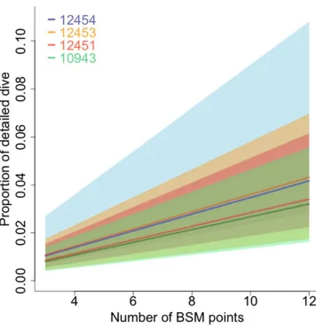
and depends on dive duration. Overall, the proportion of a dive represented by its 439
abstracted profile is very low, starting at 1% with three breakpoints and reaching 4% 440
with twelve, and increases by a constant 0.33% for each breakpoints added (Table 441
2). The mean relationship was similar for all animals but there were differences in the 442
variability in the relationship (Figure 4). 443
444
2) Variability between the samples of abstracted and detailed dives was expected, 445
due to individual variability and the different regions where data were collected. 446
not suggest any striking differences (Appendix S2, Figures S2.1 and S2.2, 448
Supplementary material). 449
450
3) Even though the detailed trajectory cannot be recovered unless the device is 451
physically recovered, the order in which breakpoints were added to the profile and 452
the 100% confidence limits to the detailed profile, which we call the dive zone, can 453
be calculated from abstracted dives. This makes it possible to derive the DZI (Figure 454
3). 455 456
4) The derivation of the DZI is based on the maximum depth of the dive, its duration 457
and the upper and lower limits to the dives zone. 458
459
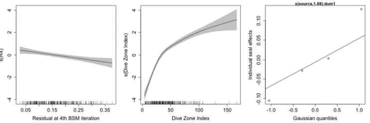
5) There was a strong, positive relationship between the RSS and the DZI together 460
with R4. We found that the DZI, R4 and a random effect for individual explained 69% 461
of the variability in the RSS for abstracted profiles with six breakpoints (deviance 462
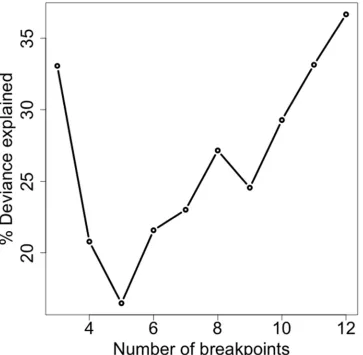
explained) (Figure 5). On its own, the DZI explained a variable proportion of 463
deviance for abstracted dives with differing numbers of breakpoints, but there was an 464
overall positive relationship with increasing breakpoints for dives with four or more 465
breakpoints (Figure 6). The DZI varied substantially between dive type and had an 466
increasing relationship with R4 (Figure 7). The dive type associated with the biggest 467
DZI values were square dives (SQ) and both V-shaped (V) and drift dives (DR) had 468
the smallest DZI, under the model (Figure 8). Dive type and R4 together explained 469
65% of the variability in the DZI (deviance explained), having accounted for 470
individual variability by fitting a random effect for individual. 471
DISCUSSION
473Change-points models are used in many fields, from neuroscience and epidemiology 474
to genetics and finance, to identify changes in time-series. One of these, the BSM, 475
was adopted on board CTD-SRDLs, as a working solution to the problem of linearly 476
approximating a non-linear path in the vertical dimension with as little information as 477
possible, while aiming to retain biologically relevant content. Until now, the 478
approximation error associated with abstracted profiles had not been investigated. 479
We provide a way of calculating and summarizing the error associated with dive 480
profiles derived using the BSM, in order to assess the information content of 481
abstracted dives. Our results suggest that BSM-abstracted dive profiles do, in fact, 482
retain enough information to estimate goodness-of-fit of the abstracted profile to the 483
detailed profile. The strong, positive relationship between the DZI and R4, and the 484
RSS is evidence for this. It means that researchers using BSM-abstracted dive 485
profiles to make inference about animal behaviour and diving ecology can now 486
calculate the DZI and R4 and incorporate a relative measure of error into their 487
analyses. 488
489
With the BSM, as with other linear approximation methods, the number of iterations 490
is critical to the quality of the abstracted dive. Our results confirm the findings of a 491
preliminary investigation during tag development, regarding the adequacy of different 492
numbers of iterations, that resulted in the standard use of four iterations of the 493
algorithm for dives collected by CTD-SRDLs. That study found that the information 494
gained in the transmission of a fifth breakpoint is relatively small, and that it would be 495
more useful to receive a measure of the variance of the detailed dive, either for the 496
paper. 498
499
It is worth noting that although the BSM can efficiently summarise a curvilinear 500
trajectory, using a piecewise-linear shape, profiles resulting from low iteration 501
numbers, may mask important biological features even if they closely approximate 502
the detailed trajectory. Our methods do not provide means for assessing the 503
biological content of abstracted dives, since the detail lost, however small, might be 504
the most biologically interesting. For example, a useful feature of the BSM is that it is 505
efficient at identifying long sections where the trajectory has low variability. In the 506
case of dives, these are often the descent and ascent phases, leaving only two 507
points to confer information about the bottom phase of the dive, which is arguably 508
the most interesting biologically. Dives with low variability in change in depth in the 509
bottom phase, also have the lowest DZI, as we found here for drift dives (DR type). 510
However, when classifying abstracted dives with a method like a random forest 511
algorithm, ancillary behavioural data are necessary for validating classes as being 512
functionally distinct, in addition to being phenomenologically distinct. 513
514
Large numbers of dive profiles are collected using CTD-SRDLs from many different 515
species (over 21 million profiles since 1991, SMRU 2012, unpublished data) and 516
used to make inferences about the biology and behaviour of the instrumented 517
animals. It seems essential that a method for assessing the accuracy of these 518
abstracted dives, at least statistically if not biologically, is made widely available. The 519
methods we have presented here make that possible. They also provide a way of 520
carrying out a “pilot” analysis when detailed dive data are available. The differences 521
breakpoints appropriate for the questions being asked. When detailed dive data are 523
available, the result of dive abstraction with different number of iterations can be 524
investigated to achieve the best result for a specific study, prior to deployment. 525
Together, these uses for our methods may help make more robust the behavioural 526
conclusions we can draw from telemetry data. 527
528
More generally, through this work we have developed a method for quantifying 529
uncertainty in the fitted values for BSMs, when the original time-series is no longer 530
available. This method could be applied to any situation where the original time-531
series data are not longer available. This could be useful in situations where large 532
amounts of data are being generated and cannot be stored or transmitted at the 533
original resolution. We demonstrate that measures of fit like the DZI and R4 have a 534
strong correspondence to the RSS and could therefore be used instead. 535
536
ACKNOWLEDGEMENTS
537This work was supported by SMRU Ltd (now SMRU Marine) in the form of a PhD 538
fellowship (T.P.). Completion of the manuscript was supported by a National 539
Research Foundation Scarce Skills Postdoctoral Fellowship at the University of 540
Cape Town, South Africa (T.P.). The CTD-SRDL data presented in this manuscript 541
were collected as part of a project funded by the Natural Environment Research 542
Council (NERC) grants NE/E018289/1 and NER/D/S/2002/00426. The authors are 543
extremely grateful for access to three high-resolution datasets from Kerguelen 544
Islands that were made available by Christophe Guinet and collected under the SO-545
MEMO framework. Fieldwork was carried out according to the Animals (Scientific 546
Animal Welfare Committee. The authors thank Martin Biuw (Akvaplan-niva, Trømso, 548
Norway) and Lars Boehme (SMRU) for use of the CTD-SRDL data, Nora Hanson 549
(SMRU) and Lars Boehme for useful comments on the manuscript, Samantha 550
Gordine (SMRU) for testing the code, and two anonymous reviewers for their 551
constructive comments on the manuscript. 552
553
DATA ACCESSIBILITY 554
• R scripts: uploaded as supporting material 555
• Example data of detailed and abstracted dive data: uploaded as supporting 556
material 557
• For access to the full datasets used in this study please contact the data 558
owners directly. South Georgia Island and Año Nuevo deployments: Mike 559
Fedak ([email protected]) and Lars Boehme (
lb284@st-560
andrews.ac.uk). Kerguelen Islands deployments: Christophe Guinet 561
([email protected]). 562
563
REFERENCES
564Aoki, K., Watanabe, Y., Crocker, D., Robinson, P.W., Biuw, M., Costa, D., Miyazaki, 565
N., Fedak, M.A. & Miller, P.J.O. (2011) Northern elephant seals adjust gliding 566
and stroking patterns with changes in buoyancy: validation of at-sea metrics of 567
body density. The Journal of experimental biology, 214, 2973–87. 568
Argos. (2011) Argos User’s Manual. URL http://wwwargos-systemorg/files/pmedia/p 569
Authier, M., Martin, C., Ponchon, A., Steelandt, S., Bentaleb, I. & Guinet, C. (2012) 571
Breaking the sticks: a hierarchical change-point model for estimating 572
ontogenetic shifts with stable isotope data. Methods in Ecology and Evolution, 3, 573
281–290. 574
Baechler, J. (2002) Dive shapes reveal temporal changes in the foraging behaviour 575
of different age and sex classes of harbour seals (Phoca vitulina). Canadian 576
Journal of Zoology, 80, 1569–1577. 577
Bailleul, F., Charrassin, J.-B., Monestiez, P., Roquet, F., Biuw, M. & Guinet, C. 578
(2007) Successful foraging zones of southern elephant seals from the 579
Kerguelen Islands in relation to oceanographic conditions. Philosophical 580
transactions of the Royal Society of London. Series B, Biological sciences, 362, 581
2169–81. 582
Beckage, B., Joseph, L., Belisle, P., Wolfson, D.B. & Platt, W.J. (2007) Bayesian 583
change-point analyses in ecology. The New Phytologist, 174, 456–67. 584
Biuw, M., Boehme, L., Guinet, C., Hindell, M., Costa, D., Charrassin, J.-B., Roquet, 585
F., Bailleul, F., Meredith, M., Thorpe, S.E., Tremblay, Y., McDonald, B., Park, 586
Y.-H., Rintoul, S.R., Bindoff, N., Goebel, M., Crocker, D., Lovell, P., Nicholson, 587
J., Monks, F. & Fedak, M.A. (2007) Variations in behavior and condition of a 588
Southern Ocean top predator in relation to in situ oceanographic conditions. 589
Proceedings of the National Academy of Sciences of the United States of 590
Biuw, M., Nøst, O., Stien, A., Zhou, Q., Lydersen, C. & Kovacs, K. (2010) Effects of 592
hydrographic variability on the spatial, seasonal and diel diving patterns of 593
southern elephant seals in the eastern Weddell Sea. PloS one, 5, 1–14. 594
Breiman, L. (2001) Random Forests. Machine Learning, 45, 5–32. 595
Campagna, C., Piola, A.R., Marin, M.R., Lewis, M., Zajaczkovski, U. & Fernández, T. 596
(2007) Deep divers in shallow seas: Southern elephant seals on the Patagonian 597
shelf. Deep Sea Research Part I: Oceanographic Research Papers, 54, 1792– 598
1814. 599
Fauchald, P. & Tveraa, T. (2003) Using first-passage time in the analysis of area-600
restricted search and habitat selection. Ecology, 84, 282–288. 601
Fedak, M.A., Lovell, P. & Grant, S. (2001) Two approaches to compressing and 602
interpreting time-depth information as collected by time-depth recorders and 603
satellite-linked data recorders. Marine Mammal Science, 17, 94–110. 604
Fedak, M.A., Lovell, P., McConnell, B. & Hunter, C. (2002) Overcoming the 605
constraints of long range radio telemetry from animals: getting more useful data 606
from smaller packages. Integrative and comparative biology, 42, 3–10. 607
Hebblewhite, M. & Haydon, D.T. (2010) Distinguishing technology from biology: a 608
critical review of the use of GPS telemetry data in ecology. Philosophical 609
transactions of the Royal Society of London. Series B, Biological sciences, 365, 610
Hindell, M., Slip, D. & Burton, H. (1991) The diving behaviour of adult male and 612
female southern elephant seals, Mirounga leonina (Pinnipedia : Phocidae). 613
Australian Journal of Zoology, 39, 595–619. 614
Jonker, F. & Bester, M. (1998) Seasonal movements and foraging areas of adult 615
southern female elephant seals, Mirounga leonina, from Marion Island. Antarctic 616
Science, 10, 21–30. 617
Liaw, A. & Wiener, M. (2002) Classification and regression by randomForest. R 618
News, 2, 18–22. 619
MacArthur, R. (1957) On the relative abundance of bird species. Proceedings of the 620
National Academy of Sciences of the United States of America, 43, 293–295. 621
MacArthur, R. & MacArthur, J. (1961) On bird species diversity. Ecology, 42, 594– 622
598. 623
McConnell, B., Chambers, C. & Fedak, M.A. (1992) Foraging ecology of southern 624
elephant seals in relation to the bathymetry and productivity of the Southern 625
Ocean. Antarctic Science, 4, 393–398. 626
McConnell, B., Fedak, M.A., Lovell, P. & Hammond, P. (1999) Movements and 627
foraging areas of grey seals in the North Sea. Journal of Applied Ecology, 36, 628
573–590. 629
McKellar, a. E., Langrock, R., Walters, J.R. & Kesler, D.C. (2014) Using mixed 630
hidden Markov models to examine behavioral states in a cooperatively breeding 631
Photopoulos, T. (2007) Behavioural Changes of a Long-Ranging Diver in Response 633
to Oceanographic Conditions. University of St Andrews. 634
R Core Team. (2013) R: A language and environment for statistical computing. R 635
Foundation for Statistical Computing. 636
Rual, P. (1989) For a better XBT bathy-message on board quality control, plus a new 637
data reduction method. Western Pacific International Meeting and Workshop on 638
Toga Coare (eds J. Picaut, R. Lukas & T. Delcroix), pp. 823–833. Noumea, New 639
Caledonia. 640
Schreer, J., Kovacs, K. & O’Hara Hines, R. (2001) Comparative diving patterns of 641
pinnipeds and seabirds. Ecological Monographs, 71, 137–162. 642
Schreer, J. & Testa, J. (1996) Classification of Weddell seal diving behavior. Marine 643
Mammal Science, 12, 227–250. 644
Thums, M., Bradshaw, C.J.A. & Hindell, M.A. (2008) A validated approach for 645
supervised dive classification in diving vertebrates. Journal of Experimental 646
Marine Biology and Ecology, 363, 75–83. 647
Toms, J. & Lesperance, M. (2003) Piecewise regression: a tool for identifying 648
ecological thresholds. Ecology, 84, 2034–2041. 649
Wood, S.N. (2000) Modelling and smoothing parameter estimation with multiple 650
quadratic penalties. Journal of the Royal Statistical Society: Series B (Statistical 651
Wood, S.N. (2011) Fast stable restricted maximum likelihood and marginal likelihood 653
estimation of semiparametric generalized linear models. Journal of the Royal 654
Statistical Society: Series B (Statistical Methodology), 73, 3–36. 655
Figures and Tables
Table 1. Deployment information and morphometrics for the detailed datasets from a northern and three southern elephant seal (a
sample of 60 study dives was taken from the dive record of each seal), and the abstracted dataset(s) from 45 southern elephant
seals. For “ct” deployments, length is given as the mean (standard error) of all animals of each sex. For deployments 12454,
12453, 12451, two length measurements were available for each animal, so we present the mean (standard error) of the two
measurements. Only one length measurement was made during deployment 10943.
Deployment Species Deployment location Period (UTC) Sampling regime Morphometrics Sex Dive duration
10943 M. angustirostris
1 adult male Año Nuevo CA, USA
23/08/2008 to 16/02/2009
Time and depth every 4s **
Length: 350.0 cm
Axial Girth: 295.0 cm M 24.95 min (0.77)
12454 M.leonina
1 adult female Kerguelen Islands
30/10/2012 to 15/02/2013
Time and depth every 4s
Length: 235.5.0 cm (6.5)
Weight: 258 kg F 19.18 min (0.63)
12453 M.leonina
1 adult female Kerguelen Islands
20/10/2012 to 11/02/2013
Time and depth every 4s
Length: 271.5 cm (6.5)
Weight: 425 kg F 23.48 cm (0.67)
12451 M.leonina
1 adult female Kerguelen Islands
30/10/2012 to 15/02/2013
Time and depth every 4s
Length: 234.0 cm (1.0)
Weight: 275 kg F 18.52 min (0.64)
ct1 M. leonina 6 adult females
Husvik,
South Georgia Island
06/01/2004 to
25/08/2004 CTD_GEN_07B* Length: 242.5 cm (6.7) F 23.96 min (0.07)
ct8
M. leonina 7 adult females 4 adult males
Husvik,
South Georgia Island
13/01/2005 to
31/10/2005 CTD_GEN_07B
Length: 255.7 cm (2.0) Length: 301.3 cm (8.5)
F
M 36.59 min (0.25)
ct40
M. leonina 5 adult females 5 adult males
Husvik,
South Georgia Island
28/01/2008 to
09/12/2008 CTD_GEN_07B
Length: 250.5 cm (13.0) Length: 343.6 cm (24.4)
F
M 27.47 min (0.38)
ct45 M. leonina 10 adult females
Husvik,
South Georgia Island
17/10/2008 to
01/02/2009 CTD_GEN_07B Length: 248.7 cm (2.9) F 19.77 min (0.18)
ct49
M. leonina 11 adult females 1 adult male
Husvik,
South Georgia Island
28/01/2009 to
12/01/2010 CTD_GEN_07B
Length: 240.5 cm (4.0) Length: 237.00 cm
F
ct58 M. leonina 13 adult females
Husvik,
South Georgia Island
22/10/2009 to
05/02/2010 CTD_GEN_07B Length: 249.5 cm (3.2) F 18.97 min (0.19) * CTD_GEN_07B is the parameter specification with which the instruments were programmed.
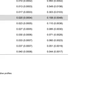
Table 2. Observed mean proportion of detailed depth samples from individuals 10943, 12454, 12453, 12451 represented by an
abstracted profile of a given number of BSM points (standard error, SE), and mean DZI (standard error, SE). The grey row
highlights the case of a dive profile with 6 points, produced by 4 iterations of the BSM.
Number of BSM points
Mean proportion of depth samples represented by
abstracted profile (SE)
Mean DZI (SE)
3 0.010 (0.0002) 0.993 (0.0002)
4 0.013 (0.0003) 0.549 (0.0156)
5 0.017 (0.0003) 0.303 (0.0103)
6 0.020 (0.0004) 0.158 (0.0048)
7 0.023 (0.0005) 0.110 (0.0036)
8 0.027 (0.0005) 0.085 (0.0030)
9 0.030 (0.0006) 0.071 (0.0026)
10 0.033 (0.0007) 0.060 (0.0023)
11 0.037 (0.0007) 0.051 (0.0019)
Figure 4. The relationship between the proportion of high-resolution time-depth samples and the number of BSM points in the abstracted dive profiles of 240 case study dives from a northern elephant seal and three southern elephant seals (see Table 1). Abstracted profiles with 3-12 points in total were generated for each
of the study dives and compared with the full resolution profile. The coloured areas incudes minimum and maximum observed range of the relationship for each individual.
Figure 5. Smooth functions of the covariates in a Generalized Additive Model with log(RSS) as the response, DZI a smooth covariate, and individual dive as a random effect. The data used to fit this model were abstracted dive profiles of 4,000 study dives from 45 southern elephant seals instrumented at South Georgia
Figure 6. The relationship between the percentage of deviance explained by a model for RSS with DZI as the explanatory variable and individual seal as a random effect, and the number of breakpoints in the dives
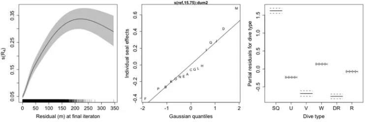
Figure 7. Smooth functions of the covariates in a Generalized Additive Model with dive zone index as the response, dive type as a factor variable, the residual as the final iteration of the BSM as a smooth covariate,
and individual seal as a random effect. The data used to fit this model were abstracted dive profiles of 22,305 study dives from 17 southern elephant seals instrumented at South Georgia Island in 2004 and
Figure 8. The fitted relationship between the dive zone index (DZI) and the residual at the final interaction of the broken stick model (R4) for each dive type. These are the predictions based on a Generalized Additive
Model, with R4 as smooth covariate, dive type as a factor variable, and individual seal as a random effect. The data used to fit this model were abstracted dive profiles of 22,305 study dives from 17 southern