A camera calibration method for a hammer throw analysis tool

(1)

A camera calibration method for a hammer throw analysis

tool

KELLEY, John <http://orcid.org/0000-0001-5000-1763>

Available from Sheffield Hallam University Research Archive (SHURA) at:

http://shura.shu.ac.uk/8188/

This document is the author deposited version. You are advised to consult the

publisher's version if you wish to cite from it.

Published version

KELLEY, John (2014). A camera calibration method for a hammer throw analysis

tool. In: JAMES, David, CHOPPIN, Simon, ALLEN, Tom and FLEMMING, Paul,

(eds.) The Engineering of Sport 10. Procedia Engineering, 10 (72). Elsevier, 74-79.

Copyright and re-use policy

See http://shura.shu.ac.uk/information.html

(2)

Procedia Engineering 72 ( 2014 ) 74 – 79

(http://creativecommons.org/licenses/by-nc-nd/3.0/).

Selection and peer-review under responsibility of the Centre for Sports Engineering Research, Sheffield Hallam University doi: 10.1016/j.proeng.2014.06.002

ScienceDirect

The 2014 conference of the International Sports Engineering Association

A camera calibration method for a hammer throw analysis tool

John Kelley

a,

*

a_{Centre for Sports Engineering Research, Sheffield Hallam University, Collegiate Crescent, Sheffield, S10 2BP, UK}

Abstract

The hammer throw in athletics has been the subject of published research since the 1980s. This has focused on case studies of individual athletes or small cohorts and has identified a number of key performance indicators such as the speed profile of the hammer during the wind-up phase. To use these key performance indicators with current athletes a bespoke analysis tool is required for frequent data collection. An unobtrusive two cameras system was proposed and a non-standard planar calibration method that allows the safety cage to remain in place was designed. The performance of the non-standard calibration method was compared to the standard calibration method using simulated data. The non-standard method was found to be suitable when intrinsic camera parameters were not recomputed. The method is a suitable alternative for volumes that cannot easily be accessed with a calibration object or volumes that are too large for practically sized calibration objects

Selection and peer-review under responsibility of the Centre for Sports Engineering Research, Sheffield Hallam University.

Keywords: camera calibration; kinematic; hammer throw; sport; 3-dimensional; performance analysis

1.Introduction

The hammer throw in athletics has been the subject of a number of 3-dimensional (3D) kinematic studies since the 1980s. Dapena (1984) investigated the effect of gravity on the speed of the hammer during the wind-up phase. Dapena (1986) and Murofushi et al. (2007) investigated the movement of both the athlete and the implement during the throw using small cohorts of athletes. These are three of several studies into elite hammer throwing that have all been limited to case studies of a small number of athletes and based on only 1 or 2 throws for each athlete.

* Corresponding author. Tel.: +44 (0)114 225 3987; fax: +44 (0)114 225 4356. E-mail address: [email protected]

(3)

75 John Kelley / Procedia Engineering 72 ( 2014 ) 74 – 79

This is because there is no bespoke system for measuring the desired parameters. Despite the limitations, these studies have provided great insight into the technical aspect of the Hammer throw including the identification of key performance indicators such as the ‘radius of rotation’, the hammer speed profile and the ‘plane of inclination’ of the hammer during the ‘wind up phase’.

Frequent data collection is required to use these key performance indicators to a) benchmark athletes, b) fully analyse the effect of training interventions (e.g. strength and condition training) and c) assist an athlete during rehabilitation after injury. The previous studies have used lab-based motion capture systems or standard 3D kinematic techniques such as direct linear transform (DLT) combined with manual digitisation to calculate the 3D position of the hammer and biomechanics of the athlete. These methods are not suitable for frequent data collection; a bespoke system is required and it is proposed that a two camera video analysis system is developed. Such a system requires:

x A stereo camera calibration method to allow the reconstruction of 3D points that is easy to implement in a hammer throwing environment

x A method for automatically digitising objects of interest such as the hammer implement

Previous 3D investigations into the hammer throw using cameras have used the DLT calibration technique. DLT calibration requires that a specific calibration object is positioned within the volume of interest (calibrated volume). For this case, the volume of interest is the throwing circle of the hammer which is within a safety cage. Filming through the safety cage would make the accurate digitisation of the calibration object impossible without removing the safety cage, which is impractical.

An alternative to DLT is planar calibration which uses a calibration board, often a checkerboard, as the calibration object. Such a technique combines two synchronised single camera calibrations (Zhang, 1999) into a stereo calibration that calculates the intrinsic camera parameters (intrinsics) and the relative position of the two cameras (extrinsics). Usually the intrinsic are recomputed using the extrinsic information during a stereo calibration to improve the accuracy of the calibration. A freely available MATLAB toolbox has been produced by Bouguet (2013) which facilitates the stereo calibration of a pair of cameras. Free, fully packaged Check3D

software is available (Goodwill, 2013) that performs automated calibrations and facilitates manual digitisation of objects and the 3D reconstruction of their position. Check3D uses the camera calibration functions from the

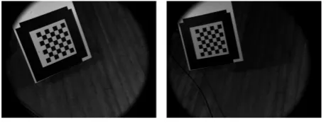
OpenCV library described by Bradski and Kaehler (2008). To complete a calibration, a series of simultaneously recorded pairs of calibration images are required. An example of a pair of calibration images from Goodwill (2013) is shown in Figure 1.

[image:3.544.158.388.437.524.2]

Fig. 1. A pair of calibration images, simultaneously recorded from the left and right camera from Goodwill (2013).

(4)

and then a number of simultaneous calibration image pairs to allow the calculation of the extrinsics. This paper will focus on comparing the standard planar calibration to the proposed non-standard method.

It is not practical to carry out multiple calibrations to compare the proposed non-standard calibration method to the described typical standard calibration method. Therefore they were compared using multiple calibrations generated from simulated calibration board positions.

2.Method

The board positions were simulated for virtual typical machine vision camera and lenses. Both cameras had a focal length of 400 pixels (approximately 10 mm for a ½ inch sensor), a resolution of 512 x 512 pixels. A small radial lens distortion effect was also simulated. The calibration board was an 8 x 8 checkerboard with the square lengths 60 mm for the standard method and 30 mm for the non-standard method. Different square sizes were used because the calibration boards are positioned much closer to the cameras for the non-standard calibration method so the checkerboard does not need to be as large. The cameras were positioned with a convergence angle of 25°. The required calibrated volume was set as a 5 x 4 m area, 3 m high with the long axis across the left camera view. This is sufficient for analyzing the wind-up phase of the hammer throw. The center of the calibrated volume was 5 m from both cameras.

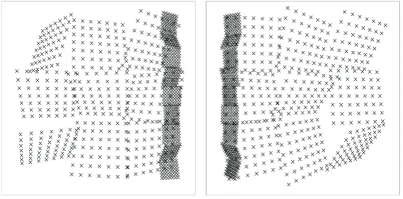
For the standard calibrations, the boards were positioned in a 3 x 3 x 3 pattern distributed across the calibration volume facing the left camera. The angle of the board relative to the left camera was randomly assigned for each board according to the following:

x Rotated around the horizontal axis by an angle between -45° and 45° (Figure 2a). x Rotated around the vertical axis by an angle between -45° and 20° (Figure 2b).

A visualisation of an example of a standard calibration from the view of both cameras is shown in Figure 3.

Fig. 2. (a) horizontal rotation range; (b) vertical rotation range

[image:4.544.120.409.504.645.2]

(5)

Fig. 3. An example of the simulated checkerboard images viewed from the left and right camera. The visualisation shows crosses where the checkerboard square corners are.

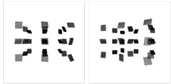
For the non-standard calibrations, the boards were positioned as follows:

x 9 boards 0.5 m away from the left camera arranged in a 3 x 3 pattern covering the field of view (not visible in the right camera)

x 9 boards 0.5 m away from the right camera arranged in a 3 x 3 pattern covering the field of view (not

visible in the left camera)

x 9 boards arranged vertically 1.5 m from both cameras (visible in both cameras)

The calibration boards were randomly rotated relative to the left camera, similarly to the calibration boards in the standard method. For the single camera calibration images, the magnitude of the rotation was between -45° and 45° for both the horizontal and vertical rotation axes. For the final 9 images visible in both cameras the boards were:

x rotated around the horizontal axis by an angle between -30° and 30° x rotated around the vertical axis by an angle between -30° and 5°

A visualisation of an example of a standard calibration from the view of both cameras is shown in Figure 4.

[image:5.544.130.415.260.401.2]

Fig. 4. An example of the simulated checkerboards viewed from the left and right camera for the non-standard calibrations. The visualisation shows crosses where the checkerboard square corners are. Only the smaller (further away) boards are visible in both cameras.

Once the board positions and orientations were determined, random noise was added to both the horizontal and vertical position of each point on each board to simulate typical error in the automatic calibration process. The noise had a mean of zero and a standard deviation of 0.1 pixels. The calibration was then carried out using the calibration module from Check3D. The module was modified to allow the non-standard calibration method, still using the functions from the OpenCV library.

Four sets of calibrations were generated; the standard method without recomputed intrinsics, the standard method with recomputed intrinsics, the non-standard method without recomputed intrinsics and the non-standard method with recomputed intrinsics. For each set, 10,000 calibrations were generated and the quality of the 3D reconstruction using each one was assessed. This was done using 693 points distributed throughout the volume at 0.5 m intervals. These 3D points have corresponding 2D image positions (UV points) in each camera image. Each calibration was used to reconstruct the 3D points from the UV points. The relative distance between each neighbouring reconstructed point was calculated and subtracted from 0.5 m. The mean relative reconstruction error (MRRE) for a calibration is the mean of this for all of the relative distances. The variance of the relative reconstruction error (VRRE) for a calibration is the corresponding variance.

(6)

consistently across the calibrated volume. The mean MRRE, the mean VRRE and the distribution of the MRRE for each set is used to compare them.

3.Results

The mean MRRE and mean VRRE are shown in Table 1. The standard method with recomputed intrinsics and the non-standard method without recomputed intrinsics are comparable with the former having a lower mean VRRE than the latter. By comparison, the standard method without recomputed intrinsics has a large mean VRRE value and the non-standard method with recomputed intrinsics has large mean MRRE and mean VRRE values.

Table 1. The mean MRRE and the mean VRRE for each calibration set.

Standard Standard Recomp. Non-Standard Non-Standard Recomp.

Mean MRRE 0.15 mm 0.01 mm 0.03 mm -19.87 mm

Mean VRRE 658.34 mm2 _{3.04 mm}2 _{5.60 mm}2 _{314.67 mm}2

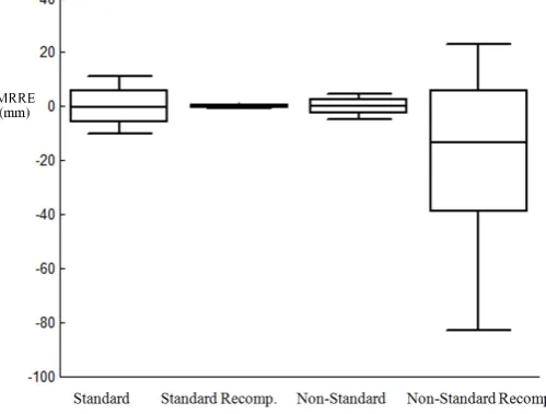
[image:6.544.140.390.345.534.2]

The distributions of the MRRE values for each calibration set (figure 5) illustrate that while the mean MRRE values for the first three sets were similar in Table 1, the distributions are not. The MRRE values are very close to 0 for all of the standard calibrations with recomputed intrinsics. The MRRE values vary slightly more for the non-standard method without recomputed intrinsics and much more for the non-standard method without recomputed intrinsics.

Fig. 5 The distribution of the MRRE for each set of calibrations showing the median, upper and lower quartiles and upper and lower deciles.

4.Discussion

(7)

recomputed intrinsics has a large negative mean MRRE and a widely spread distribution of MRRE values which indicates that the calibrations are likely to have a large error and not be repeatable between calibrations.

Both the standard method with recomputed intrinsics and the non-standard method without recomputed intrinsics have low mean VRRE. This indicates that a calibration using either method is likely to be consistent across the calibrated volume. Both the standard method without recomputed intrinsics and the non-standard method with recomputed intrinsics have high mean VRRE so will produce calibrations that are likely to be inconsistent across the calibrated volume.

A calibration using the standard method with recomputed intrinsics is likely to produce low errors, be repeatable and be consistent across the calibrated volume. A calibration using the non-standard method without recomputed intrinsics is comparable. However, such a calibration will be less repeatable and may be less consistent across the calibrated volume. Re-computing the intrinsics for the non-standard method produces much worse calibrations. This is likely to be because the re-computation process is not designed to be used with such a non-standard calibration method so does not assign enough importance to the calibration boards visible in only one camera.

5.Conclusion

The intrinsics should not be recomputed for the proposed non-standard calibration method. The reconstruction using the non-standard calibration method is much more accurate than the standard method without re-computed intrinsics. The reconstruction is less accurate than, but comparable to, the standard method with re-computed intrinsics. The non-standard calibration method provides a usable alternative to the standard method when access to the calibrated volume is not possible. An additional advantage is that the calibration board can be smaller because it is held much closer to the camera. This may also be of use for large calibration volumes where the board size required would be impracticable large.

The proposed non-standard calibration method is suitable for use in an analysis tool for the hammer. The presented results can be used to guide how the described hammer trajectories are compared and presented, tempering results with quantified possible error.

References

Bouguet, J. 2013. Camera Calibration Toolbox for Matlab. Available at: www.vision.caltech.edu/bouguetj/calib_doc/ [Accessed October 1, 2013].

Bradski, G, Kaehler, A. 2008. Camera Models and Calibration. In: Learning OpenCV: Computer Vision with the OpenCV Library. O’Reilly Media, 370–404

Dapena, J. 1984. The pattern of hammer speed during a hammer throw and influence of gravity on its fluctuations. Journal of biomechanics, 17(8), 553-559.

Dapena, J. 1986. A kinematic study of center of mass motions in the hammer throw. Journal of biomechanics, 19(2), 147-158. Goodwill, S. 2013. Check3D – camera calibration tool for 3D analysis. Available at: www.check3d.co.uk/ [Accessed October 1, 2013]. Murofushi, K., Sakurai, S., Umegaki, K., & Takamatsu, J. 2007. Hammer acceleration due to thrower and hammer movement patterns. Sports

Biomechanics, 6(3), 301-314.