Robust Automatic Methods for Outlier and
Error Detection
Ray Chambers, Adão Hentges and Xinqiang Zhao
Abstract
Editing in surveys of economic populations is often complicated by the fact that outliers due to errors in the data are mixed in with correct, but extreme, data values. In this paper we describe and evaluate two automatic techniques for error identification in such long tailed data distributions. The first is a forward search procedure based on finding a sequence of error-free subsets of the error contaminated data and then using regression modelling within these subsets to identify errors. The second uses a robust regression tree modelling procedure to identify errors. Both approaches can be implemented on a univariate basis or on a multivariate basis. An application to a business survey data set that contains a mix of extreme errors and true outliers is described.
ROBUST AUTOMATIC METHODS FOR OUTLIER AND
ERROR DETECTION
Ray Chambers(1), Adão Hentges(2) and Xinqiang Zhao(1)
(1) Department of Social Statistics, University of Southampton
Highfield, Southampton SO17 1BJ
(2) Departamento de Estatística, Universidade Federal do RS
Caixa Postal 15080, 91509-900 Porto Alegre RS, Brazil.
May 22, 2003
Address for correspondence: Professor R.L. Chambers
Department of Social Statistics
University of Southampton
Highfield
Southampton SO17 1BJ
Abstract: Editing in surveys of economic populations is often complicated by the fact that
outliers due to errors in the data are mixed in with correct, but extreme, data values. In this
paper we describe and evaluate two automatic techniques for error identification in such long
tailed data distributions. The first is a forward search procedure based on finding a sequence
of error-free subsets of the error contaminated data and then using regression modelling
within these subsets to identify errors. The second uses a robust regression tree modelling
procedure to identify errors. Both approaches can be implemented on a univariate basis or on
a multivariate basis. An application to a business survey data set that contains a mix of
extreme errors and true outliers is described.
Key words: Survey data editing; representative outliers; robust regression; regression tree
1. Introduction
1.1 Overview
Outliers are a common phenomenon in business and economic surveys. These are data
values that are so unlike values associated with other sample units that ignoring them can lead
to wildly inaccurate survey estimates. Outlier identification and correction is therefore an
important objective of survey processing, particularly for surveys carried out by national
statistical agencies. In most cases these processing systems operate by applying a series of
edits that identify data values outside bounds determined by the expectations of subject matter
specialists. These outlier values are then investigated further, in many cases by re-contacting
the survey respondents, to establish whether they are due to errors in the data capture process
or whether they are in fact valid. Chambers (1986) refers to the latter valid values as
representative outliers, insofar as there is typically no reason to believe that they are unique
within the survey population. Outlier values that are identified as errors, on the other hand,
are not representative, and it is assumed that they are corrected as part of survey processing.
A common class of such errors within the business survey context is where the survey
questionnaire asks for answers to be provided in one type of unit (e.g. thousands of pounds)
while the respondent mistakenly provides the required data in another unit (e.g. single
pounds). Sample cases containing this type of error therefore have true data values inflated by
a factor of 1000. Left uncorrected, such values can seriously destabilise the survey estimates.
The standard approach to the type of situation described above is to use a large
number of edits to identify as many outliers as possible during survey processing. These
outliers are then followed up to establish their correct values. If the correct value is identical
to the value that triggered the edit failure, then this value is not an error but corresponds to a
typically one that is subjectively determined as “more typical”. In continuing surveys this can
be the previous value of the same variable, provided that value is acceptable.
There are two major problems with this approach. The first is that it can be extremely
labour intensive. This is because the edit bounds are often such that a large proportion of the
sample data values lie outside them. This leads to many unnecessary re-contacts of surveyed
individuals or businesses, resulting in an increase in response burden. Secondly, the
subjective corrections applied to representative outliers leads to biases in the survey estimates,
particularly for estimates of change. Since there are often large numbers of such
representative outliers identified by this type of strategy, the resulting biases from their
“correction” can be substantial.
This paper describes research aimed at identifying an editing strategy for surveys that
are subject to both outliers and errors that overcomes some of the problems identified above.
In particular, the aim is to develop an automated outlier identification strategy that finds as
many significant errors in the data as possible, while minimising the number of representative
outliers also identified (and whose values are therefore incorrectly changed). In particular, the
methods described below do not rely on specification of edit bounds and use modern robust
methods to identify potential errors, including outliers, from the sample data alone.
1.2 The ABI Data
This research has been carried out as part of the Euredit project (Charlton et al, 2001).
In particular, we use two data sets that were created within this project for the specific
purpose of evaluating automatic methods for edit and imputation. Both contain data for 6099
businesses that responded to the UK Annual Business Inquiry (ABI) in the late 1990s. The
they represent are data of sufficient quality for use in official statistics. The second data set
contains values for the same variables and businesses as in the first. However, these values
now include both introduced errors and missing values, and can be considered as representing
the type of “raw” data that are typically seen prior to editing. We refer to this data set as the
perturbed data below. Note that the clean data and the perturbed data contain a significant
number of common extreme values (i.e. representative outliers), reflecting the fact that the
[image:6.595.70.547.292.412.2]clean data may still contain errors.
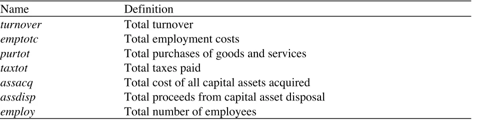
Table 1. The ABI variables
Name Definition
turnover Total turnover
emptotc Total employment costs
purtot Total purchases of goods and services
taxtot Total taxes paid
assacq Total cost of all capital assets acquired assdisp Total proceeds from capital asset disposal employ Total number of employees
Table 1 lists the names and definitions of the variables collected in the ABI that we
consider in this paper. The names are those used in the Euredit project, and these seven
variables represent the major outcome variables for the ABI. In addition we assume that we
have access to “complete” (no missing values and no errors) auxiliary information for the
sampled businesses on the Inter-Departmental Business Register or IDBR (the sample frame
for the ABI). The most important auxiliary variable is the estimated turnover of a business
(turnreg, defined in terms of the IDBR value of turnover for a business, in thousands of
pounds). Other auxiliary information on the IDBR relates to the estimated number of
employees of a business and its industrial classification. Together, these define the sampling
strata for the ABI. Below we assume that we have access to the strata affiliations of the
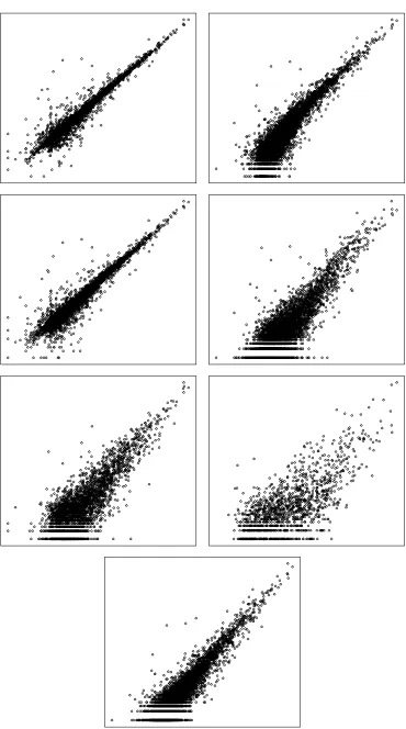
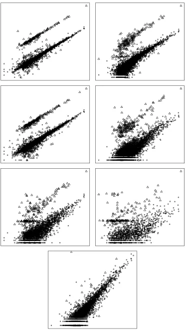
Figures 1 and 2 show the relationship between the ABI variables and the auxiliary
variable turnreg for the values contained in the clean data and the perturbed data. Because
these variables are extremely heteroskedastic, scatterplots of their raw values reveal little.
Consequently all plots in Figures 1 and 2 are on the log scale. Also, for reasons of
confidentiality, no scale is displayed on these plots. It is clear from Figures 1 and 2 that
although the general relationship between turnreg and the ABI variables is linear in the log
scale, comparison of the clean data and the perturbed data show there are a very large
number of significant errors leading to outliers (these appear as ∆’s in Figure 2, but not in
Figure 1) as well as large representative outliers (these appear in both Figure 1 and Figure 2).
Figures 1 and 2 about here
2. Outlier Identification Via Forward Search
The first automatic method we investigate was suggested by Hadi and Simonoff
(1993). See also Atkinson and Riani (2000). The basic idea is simple. In order to avoid the
well-known masking and swamping problems that can occur when there are multiple outliers
in a data set (see Barnett and Lewis 1994, Rousseeuw and Leroy 1987), the algorithm starts
from an initial subset of observations of size m < n that is chosen to be outlier free. Here n
denotes the number of observations in the complete data set. In the regression context, a
model for the variable of interest is estimated from this initial “clean” subset. Fitted values
generated by this model are then used to generate n distances to the actual sample data values.
The next step in the algorithm redefines the clean subset to contain those observations
corresponding to the m+1 smallest of these distances and the procedure repeated. The
algorithm stops when distances to all sample observations outside the clean subset are all too
In order to more accurately specify this forward search procedure, we assume values
of a p-dimensional multivariate survey variable Y and a q-dimensional multivariate auxiliary
variable X are available for the sample of size n. We denote an individual’s value of Y and X
by yi and xi respectively. The matrix of sample values of Y and X is denoted by
)
( 1 ′
= y yn
y L and x=(x1Lxn)′ respectively. We seek to identify possible outliers in y.
Generally identification of such outliers is relative to some assumed model for the
conditional expectation of Y given X. Given the linear structure evident in Figures 1 and 2,
we assume that a linear model E(Y)= ββX can be used to characterise this conditional expectation, where β = ( ′ β 1,Lβ ′ p) is a p ′ × q matrix of unknown parameters. A large residual
for one or more components of Y is typically taken as evidence that these values are outliers.
For p = 1 we let β ˆ (m) and σ ˆ (m)
2
denote the regression model parameter estimates based
on a clean subset of size m. For an arbitrary sample unit i, Hadi and Simonoff (1993) suggest
the distance from the observed value yi to the fitted value generated by these estimates be
calculated as
di(m)=
yi− ′ x iβ ˆ (m)
ˆ
σ (m) 1−λix ′ i(X ′ (m)X(m)) −1
xi
where X(m) denotes the matrix of values of X associated with the sample observations making
up the clean subset, and λi takes the value 1 if observation i is in this subset and –1 otherwise.
The clean subset of size m+1 is then defined by those sample units with the m+1 smallest
values of di(m). For p > 1, Hadi (1994) uses the squared Mahalanobis distance
Di(m)
2
=(yi −y ˆ i(m)) ˆ ′ S −(m1)(yi −y ˆ i(m))
where y ˆ i(m) denotes the fitted value for yi generated by the estimated regression models for the components of this vector, and
S ˆ (m) =(m−q)
−1
(yi−y ˆ i(m))(yi−y ˆ i(m)) ′
estimated covariance matrix of the errors associated with these models. The summation here
is over the observations making up the clean subset of size m.
For p = 1 Hadi and Simonoff (1993) suggest stopping the forward search when the
(m+1)th
order statistic for the distances di(m) is greater than the 1 – α/2(m+1) quantile of the
t-distribution on m-q degrees of freedom. When this occurs the remaining n-m sample
observations are declared as outliers. Similarly, when p > 1, Hadi (1994) suggests the forward
search be stopped when the (m+1)th order statistic for the squared Mahalanobis distances
Di2(m) exceeds the 1-α/n quantile of the chi-squared distribution on p degrees of freedom.
Definition of the initial clean subset is important for implementing the forward search
procedure. Since the residuals from the estimated fit based on the initial clean subset define
subsequent clean subsets, it is important that the parameter estimates defining this estimated
fit are unaffected by possible outliers in the initial subset. This can be achieved by selecting
observations to enter this subset only after they have been thoroughly checked. Alternatively,
we use an outlier robust estimation procedure applied to the entire sample to define a set of
robust residuals, with the initial subset then corresponding to the m observations with smallest
absolute residuals relative to this initial fit. Our experience is that this choice is typically
sufficient to allow use of more efficient, but non-robust, least squares estimation methods in
subsequent steps of the forward search algorithm.
Before ending this section, we should point out that the forward search method
described above is based on a linear model for the non-outlier data, with stopping rules that
implicitly assume that the error term in this model is normally distributed. Although Figures 1
and 2 indicate that these assumptions are not unreasonable for logarithmic transforms of the
ABI data, it is also clear that they are unlikely to hold exactly. This may not be of practical
from the normal. However, an alternative outlier detection method that does not assume either
linearity or normality would appear to be worth considering.
3. Outlier Identification Via Robust Tree Modelling
Regression tree models (Breiman et al, 1984) are now widely used in statistical data
analysis, especially in data mining applications. Here we use a tree modelling approach that is
robust to the presence of outliers in data to identify gross errors and extreme outliers. The
WAID software for regression and classification tree modelling that was used for this purpose
was developed for missing data imputation under the Autimp project (Chambers et al, 2001).
Under the Euredit project a toolkit of programs has been created that emulates and extends
the capabilities of WAID. These programs work under R (Ihaka and Gentleman, 1996).
Similar software products are CART (Steinberg and Colla, 1995), the S-PLUS (MathSoft,
1999) tree function (also available in R), the R function rpart and the CHAID program in
SPSS AnswerTree (SPSS, 1998). The code for the WAID toolkit is available from the
authors.
The basic idea behind WAID is to sequentially divide the original data set into
subgroups or nodes that are increasingly more homogeneous with respect to the values of a
response variable. The splits themselves are defined in terms of the values of a set of
categorical covariates. The categories of these covariates do not need to be ordered. By
definition, WAID is a nonparametric regression procedure. It also has the capacity to
implement outlier robust splitting based on M-estimation methodology (Huber, 1981). In this
case outliers are “locally” down-weighted when calculating the measure of within node
heterogeneity (weighted residual sum of squares) used to decide whether a node should be
split or not. The weights used for this purpose are themselves based on outlier robust
3.1 The WAID Regression Tree Algorithm For Univariate Y
This assumes a rectangular data set containing n observations, values {yi} of a
univariate response variable Y and values {
x1i,Lxpi} of p categorical covariates X1, ..., Xp. No
missing X-values are allowed in the current version of WAID. For scalar Y WAID builds a
regression tree. If Y is categorical, WAID builds a classification tree. The only difference
between these two types of trees is the heterogeneity measure used to determine tree-splitting
behaviour. Since our focus is outlier identification, we are concerned with scalar response
variables only and so we restrict consideration to WAID's regression tree algorithm.
The basic idea used in WAID (as well as other tree-based methods) is to split the
original data set into smaller subsets or “nodes” in which Y-values are more homogeneous. In
WAID this is accomplished by sequential binary splitting. At each step in the splitting
process, all nodes created up to that point are examined in order to identify the one with
maximum heterogeneity. An optimal binary split of this "parent" node is then carried out.
This is based on identifying a set of values of one of the covariates X1, ..., Xp such that a split
of the parent node into one “child” node containing only cases possessing these values and
another child node containing the remaining cases minimises the heterogeneity of these child
nodes. In searching for this optimal split, covariates are classified as monotone or
non-monotone. Candidate splits for a monotone X are determined by splits with respect to the
ordered values of X in that node. Candidate splits for a non-monotone X are defined with
respect to values of X sorted by their corresponding average Y value in the node. The splitting
process continues until a suitable stopping criterion is met. At present this is when either (i)
all candidate parent nodes are effectively homogeneous; (ii) all candidate parent nodes are too
small to split further; or (iii) a user-specified maximum number of nodes is reached. Unlike
"optimal" tree. The set of nodes defining the final tree are typically referred to as the terminal
nodes of the tree.
As the above description implies, the crucial step in the splitting process is the
calculation of the heterogeneity for a particular node. For the kth node created in the splitting
process this is the weighted sum of squared residuals
WSSRk = wik(yi−y wk)2
i∈k
∑
where i∈k denotes the cases making up the node, wik is the weight attached to ith case in the
node and y wk is the weighted mean of Y in the node,
y wk= wikyi
i∈k
∑
wiki∈k
∑
.The weight wik is calculated as the ratio
wik=
ψ(yi−y wk)
yi−y wk
where ψ(x) denotes an appropriately chosen influence function. The S-PLUS/R toolkit
version of WAID uses weights returned by the robust regression function rlm in the MASS
robust statistics library (Venables and Ripley, 1994). These weights are rescaled within
WAID to sum to the number nk of cases within node k.
3.2 The WAID Regression Tree Algorithm For Multivariate Y
Unlike other regression tree algorithms, the WAID toolkit can also build a regression
tree for a p-dimensional response variable Y, and so can be used for multivariate outlier
detection. The only difference between the univariate and multivariate tree fitting procedures
is the method used to calculate the heterogeneity of a candidate node. Three options are
available in this regard. In what follows tree “stages” are indexed by k (k = 1 corresponds to
the original data set and k = K denotes the final stage of the tree), and the candidate nodes for
Option 1: The program first grows p univariate trees, one for each component of the
response vector. Each such tree is characterised by an n × K matrix of weights, where column
k of this matrix contains the weights used to determine node heterogeneity for all nodes
defined at stage k of the tree growing procedure.
Let wij
(hk)
denote the weight associated with case i in node h at stage k of the univariate
tree defined by response variable j. WAID then builds a tree using the heterogeneity measure
for candidate node h at stage k of the multivariate tree:
WRSShk = wij(hk)(y
ij−y whj
(k))2
j=1
p
∑
i∈h
∑
where
y whj(k) = wij(hk)yij
i∈h
∑
wij(hk)i∈h
∑
.We can think of this as an “average heterogeneity” approach. Note that it is not scale invariant
– a component response variable that is much larger in scale than the other component
response variables will dominate this heterogeneity measure and hence dominate the tree
growing process. Consequently component variables that differ wildly in terms of scale
should be first rescaled before this option is used to build a multivariate tree.
Option 2: Here again WAID grows p univariate trees to obtain the weights wij(hk).
However, in this case the measure of heterogeneity for candidate node h at stage k in the
multivariate tree is
WRSSk= wi(hk) (y
ij−y whj
(k))2
j=1
p
∑
i∈h
∑
where
y whj(k) = wi(hk)yij
i∈h
∑
wi(hk)i∈h
∑
and
We can think of this approach as an “average weight” approach. It also is not scale invariant.
Option 3: This is the only truly multivariate tree growing option in WAID. The
weight associated with observation i in candidate node h at stage k is calculated iteratively as
wi(hk)=ψ yi−y wh (k)
wh
(
)
yi−y wh(k)
wh
where yi denotes the p-vector of response values for this case, y wh(k)= w
i
(hk)y
i i∈h
∑
wi(hk)i∈h
∑
,the function ψ corresponds to an influence function and yi−y wh(k)
wh = swhj
−2
(yij −y whj(k))2
j=1
p
∑
,where swhj2 = wi (hk)
(yij−y whj(k))2
i∈h
∑
wi(hk)
i∈h
∑
.3.3 Outlier Identification Using WAID
Each time WAID splits the data set to create two new nodes it creates a new set of
weights for the cases making up those nodes. When these weights are based on a robust
influence function, outliers within the node have weights close to zero and non-outliers have
weights around one. These weights reflect distance from a robust estimate of location for the
values in the node. Consequently a value that is not immediately identifiable as an outlier
within larger nodes created earlier in the tree building process is more likely to become
identified as such as it is classified into smaller and smaller nodes. In effect, the weights
associated with such cases tend to move towards zero. Conversely, extreme points in the
covariate space with corresponding extreme Y values are initially given small weights.
However, such points are quickly isolated into terminal nodes in the tree splitting process, at
which point the weights associated with these points increase back to values near one.
The WAID outlier identification algorithm defines an outlier as a case with an average
one that successfully identifies outliers due to errors while minimising identification of “true”
(i.e. representative) outliers. Let Nerrors equal to the total number of true errors in the data, and,
for a given threshold w, put Noutliers(w) equal to the total number of outliers identified by
WAID on the basis of the specified threshold w, nerrors(w) equal to the corresponding number
of errors identified as outliers, and nnon-errors(w) equal to the total number of non-errors
identified as outliers. The proportion of error-generated outliers identified by WAID is
R1(w)= nerrors(w) Nerrors
while the proportion of non-errors identified as outliers using the threshold w is
R2(w)= nn on−errors(w) Noutliers(w) =1−
nerrors(w)
No utliers(w).
The optimal threshold value is then
w*=arg max
w [R1(w)(1−R2(w))].
4. Identifying Errors And Outliers In The Perturbed Data
4.1 Error Detection Using Forward Search
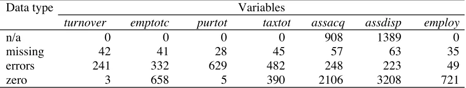
Table 2 shows the incidence of errors and missing values for each of the ABI variables
in the perturbed data. It also shows the incidence of “n/a” codes for these variables
(indicating no response was required for that variable for a sampled business) and the
incidence of zero values. Note the large number of zero values for the assdisp and assacq
[image:15.595.65.520.666.752.2]variables.
Table 2. Incidence of incorrect and non-standard data types in the perturbed data.
Data type Variables
turnover emptotc purtot taxtot assacq assdisp employ
n/a 0 0 0 0 908 1389 0
missing 42 41 28 45 57 63 35
We first applied the forward search algorithm described in Section 2 to these data
treating each variable separately (i.e. a univariate forward search). In each case we fitted a
linear model in the logarithm of the variable concerned, using the logarithm of turnreg as the
covariate. Two types of model were investigated. The first (across stratum) was fitted using
all cases in the data set. The second (stratum level) fitted a separate linear model within each
sampling stratum in the data set. Cases with zero, n/a or missing values were excluded from
the outlier search procedure. As described in Section 2, the initial subset for the forward
search procedure was defined by the smallest absolute residuals from a robust regression fit to
the entire data set. This regression fit was based on the bisquare influence function
ψ(t)=t(1−min(1,t2/c2))2, with c = 4.685. The size of this initial data was set at 70 per cent of
the size of the overall data set, since smaller initial data sets greatly increased the execution
time of the algorithm and led to no change in the set of identified outliers. The stopping rule
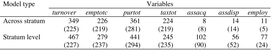
suggested by Hadi and Simonoff (1993) was used, with α = 0.01. Table 3 shows the results
from this univariate outlier search. On the basis of these results the across stratum
specification of the regression model used in the forward search seems preferable for the ABI
[image:16.595.71.539.559.647.2]data.
Table 3. Numbers of outliers detected (with numbers of errors detected in parentheses)
using univariate forward search applied to the perturbed data.
Model type Variables
turnover emptotc purtot taxtot assacq assdisp employ Across stratum 349
(225) 226 (219) 361 (281) 224 (219) 8 (8) 14 (14) 11 (5) Stratum level 467
(227) 279 (237) 441 (294) 245 (235) 102 (90) 56 (52) 77 (24)
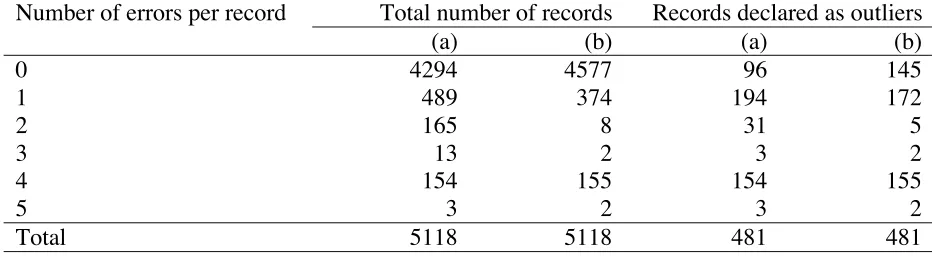
A multivariate forward search was also carried out. In this case we restricted attention
to the 5118 cases where turnover, emptotc, purtot, taxtot and employ were all strictly positive.
We excluded the variables assacq and assdisp from consideration because the large number
values for all seven variables. In the columns labelled (a) in Table 4 we show the number of
cases with errors detected by this method distributed according to the number of errors in
each case. We see that out of a total of 824 cases with one or more errors, the multivariate
forward search detected 385. It also identified 96 cases with no errors as outliers. If we
restrict attention to those cases with “significant” errors in one or more of turnover, emptotc,
purtot, taxtot and employ, i.e. those cases where the perturbed values of these variables differ
by more than 100 per cent from their values in the clean data, then we obtain the results
shown in the columns labelled (b) in Table 4. In this case the multivariate forward search
[image:17.595.63.534.377.506.2]procedure finds 336 out of the 541 cases with at least one “significant” error.
Table 4. Error detection performance of multivariate forward search procedure (across
stratum model) applied to perturbed data. Numbers in columns labelled (a) refer to all
cases, while numbers in columns labelled (b) refer to cases with “significant” errors.
Number of errors per record Total number of records Records declared as outliers
(a) (b) (a) (b)
0 4294 4577 96 145
1 489 374 194 172
2 165 8 31 5
3 13 2 3 2
4 154 155 154 155
5 3 2 3 2
Total 5118 5118 481 481
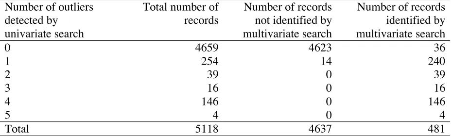
In Table 5 we contrast the performance of the multivariate forward search with that of
the individual univariate forward search procedures. In both cases the across stratum version
of the model was used in the forward search procedure. Here we see that 36 records were
identified as outliers by the multivariate search and were not identified as such by any of the
univariate searches. Furthermore only 14 records were identified by one of the univariate
searches as containing an outlier and were not identified as such by the multivariate search.
All records containing two or more outliers (as identified by the univariate searches) were
Table 5. Comparing the outlier detection performances of the univariate and
multivariate forward searches (across stratum model) applied to the perturbed data.
Number of outliers detected by
univariate search
Total number of records
Number of records not identified by multivariate search
Number of records identified by multivariate search
0 4659 4623 36
1 254 14 240
2 39 0 39
3 16 0 16
4 146 0 146
5 4 0 4
Total 5118 4637 481
Given that the multivariate forward search is restricted to cases where all components
are non-zero, and given the lack of a strong differentiation in the performance of these two
methods with the perturbed data, we restrict attention to comparisons with the univariate
forward search method in what follows.
4.2 Error Detection Using WAID
Initially we focus on a univariate approach, building robust trees for the individual
variables in Table 1. To save space we provide results below only for turnover, emptotc and
assacq, since these are representative of the results obtained for the other variables. In all
cases we built trees for the logarithm of the variable value. As in the previous section, cases
with zero, n/a or missing values were excluded from the tree building process. All trees used
the register variable turnreg, categorised into its percentile classes, as the covariate. This
covariate was treated as monotone in the tree building process and each tree was built using
the default option of robust splitting based on the bisquare influence function (c = 4.685). All
trees were grown to 50 terminal nodes, with no node containing less than 5 cases.
Comparison of the trees grown using the clean data and the perturbed data showed
no impact on the tree growing process. Furthermore, these trees were substantially different
from corresponding non-robust trees (ψ(t)=t) grown from these data sets.
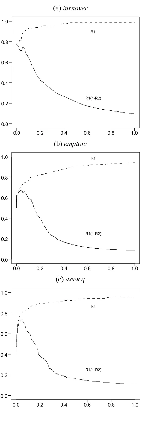
Figure 3 shows the plots of R1(w) and R1(w)(1-R2(w)) generated by these trees for the
variables turnover, emptotc and assacq. We see that for all three variables, R1(w)(1-R2(w))
attains a maximum early, then falls away steadily. This behaviour is reflected in the plots for
R1(w), which shows that most of the errors in these variables are detected using small values
of w, with few non-errors detected at the same time. As w increases the remaining errors are
then gradually detected, at the cost of identifying increasing numbers of non-errors as outliers,
evidenced by the increasing separation of R1(w) and R1(w)(1-R2(w)).
Figure 3 about here
In most cases, errors detected at larger values of w are “non-significant”, reflecting
small differences from corresponding true values. As in the previous section, we define a
“significant” error as one where the relative difference between the perturbed data value and
the clean data value is greater than one. Table 6 shows the values of R1(w) (denoted Rsig)
when only significant errors are taken into account. Observe that for all three variables over
80 per cent of such errors are identified at the optimal value w*.
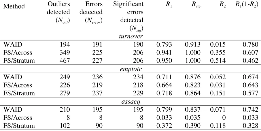
Table 6 also contrasts the performance of the WAID procedure with the corresponding
forward search procedures. Here we see that for turnover this approach does identify all the
significant errors in the data, but at the cost of identifying many more outliers than the
WAID-based procedure. Both approaches seem comparable for emptotc. However, for assacq
the WAID-based procedure is clearly superior in terms of identifying significant errors, while
at the same time keeping the number of non-errors identified as outliers to an acceptable
Table 6. Univariate WAID error detection performance (perturbed data) for turnover,
emptotc and assacq compared with the corresponding forward search (FS) performance.
Note that WAID results are for w = w*.
Method Outliers detected (Nout)
Errors detected (Nerror)
Significant errors detected (Nsig)
R1 Rsig R2 R1(1-R2)
turnover
WAID 194 191 190 0.793 0.913 0.015 0.780
FS/Across 349 225 206 0.941 1.000 0.355 0.607
FS/Stratum 467 227 206 0.950 1.000 0.514 0.462
emptotc
WAID 249 236 234 0.711 0.876 0.052 0.674
FS/Across 226 219 218 0.664 0.823 0.031 0.643
FS/Stratum 279 237 229 0.718 0.864 0.151 0.577
assacq
WAID 210 195 195 0.799 0.837 0.071 0.742
FS/Across 8 8 8 0.033 0.035 0 0.033
FS/Stratum 102 90 90 0.372 0.390 0.118 0.328
The trees used in the preceding analysis all had 50 terminal nodes. A natural question
to ask at this stage is therefore about the impact of tree size (as measured by numbers of
terminal nodes) on outlier identification. Rather surprisingly, at least as far as the perturbed
data is concerned, tree size turns out to have little impact. Table 7 shows the performance
characteristics of trees of varying size for turnover and assacq. Provided a tree has 10 or more
terminal nodes, there is little to be gained by increasing the size of the tree.
Table 7. Impact of tree size (numbers of terminal nodes) on outlier and error detection
performance with the perturbed data. In all cases the optimal value w* was used.
Size wopt Nout Nerror Nsig R1 Rsig R2 R1(1-R2) turnover
5 0.00001 206 189 188 0.784 0.904 0.083 0.720
10 0.00161 195 191 190 0.793 0.913 0.021 0.776
25 0.00075 194 191 190 0.793 0.913 0.015 0.780
50 0.00053 194 191 190 0.793 0.913 0.015 0.780
100 0.00053 194 191 190 0.793 0.913 0.015 0.780
assacq
5 0.03600 213 187 187 0.766 0.803 0.122 0.673
10 0.05009 226 195 195 0.799 0.837 0.137 0.690
25 0.04525 211 195 195 0.799 0.837 0.076 0.739
50 0.04464 210 195 195 0.799 0.837 0.071 0.742
[image:20.595.60.534.571.762.2]So far we have investigated the performance of univariate trees for outlier and error
detection. We now consider the use of a multivariate tree for the same purpose. As with the
multivariate forward search procedure, we restrict attention to the five ABI variables turnover,
emptotc, purtot, taxtot and employ where excessive zero values are not a problem. Again, all
data values were transformed to the logarithmic scale.
Recollect that there are three options available for growing a multivariate tree,
corresponding to the way the “multivariate heterogeneity” associated with a particular tree
split is defined (see Section 3.2). In Figure 4 we show how the error detection performance
for the turnover variable for the three different trees generated by these options varies with w.
This clearly shows that option 1 (average heterogeneity) is the preferable approach for this
variable.
[image:21.595.85.511.473.742.2]Figure 4 about here
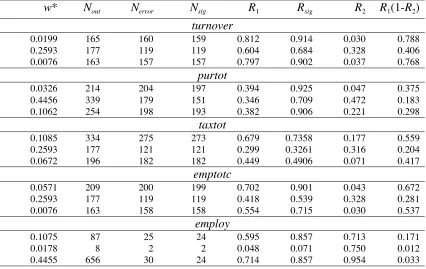
Table 8. Error detection performance for a multivariate tree based on the perturbed
data. Results for the three multivariate options, with w = w*, are set out below each
other for each variable. Note that for option 1 (first line for each variable), the optimal
value w* is the optimal univariate value.
w* Nout Nerror Nsig R1 Rsig R2 R1(1-R2) turnover
0.0199 165 160 159 0.812 0.914 0.030 0.788
0.2593 177 119 119 0.604 0.684 0.328 0.406
0.0076 163 157 157 0.797 0.902 0.037 0.768
purtot
0.0326 214 204 197 0.394 0.925 0.047 0.375
0.4456 339 179 151 0.346 0.709 0.472 0.183
0.1062 254 198 193 0.382 0.906 0.221 0.298
taxtot
0.1085 334 275 273 0.679 0.7358 0.177 0.559
0.2593 177 121 121 0.299 0.3261 0.316 0.204
0.0672 196 182 182 0.449 0.4906 0.071 0.417
emptotc
0.0571 209 200 199 0.702 0.901 0.043 0.672
0.2593 177 119 119 0.418 0.539 0.328 0.281
0.0076 163 158 158 0.554 0.715 0.030 0.537
employ
0.1075 87 25 24 0.595 0.857 0.713 0.171
0.0178 8 2 2 0.048 0.071 0.750 0.012
In Table 8 we show the error detection performance diagnostics for each of the five
component variables and for each option at the optimal value of w thus defined. This confirms
our observation above that option 1 (average heterogeneity) is preferable to the two other
multivariate options. However, comparing the results in Table 8 with those in Table 6, we see
that none of the multivariate trees perform significantly better than the corresponding
univariate trees. This is consistent with our earlier observation about the lack of a similar
improvement using the forward search approach, and indicates that, for the perturbed data at
least, virtually all the errors are in low dimensions and so are easily detected via a univariate
outlier search procedure.
5. Discussion
In this paper we compare two approaches to identification of gross errors and outliers
in survey data. The first uses a forward search procedure based on a parametric model for the
data. The second is based on a robust nonparametric modelling approach, based on regression
tree methodology. Software (WAID) for implementing this second approach is described, and
both approaches are evaluated using a realistic business survey data set created to reflect the
errors that are typically found in such data. Overall, the regression tree method performs
rather well and, for the application we consider, seems preferable to the forward search
procedure. Multivariate versions of both approaches were also evaluated. Unfortunately, the
data set we used for the application did not appear to have a significant number of truly
multivariate outliers, and so we are unable at this stage to recommend the multivariate version
of the regression tree procedure.
The regression tree approach is dependent on choice of a tuning constant,
corresponding to the optimal weight cutoff w*. In the Euredit project the value of this
This assumes that the value of w* remains the same over time. This is unlikely to be the case.
Further work therefore needs to be carried out to determine an optimum updating strategy for
this parameter.
The problem of dealing with “special” values (e.g. zero) when carrying out error
detection remains an open problem. In this paper we have implicitly assumed these values are
recorded without error. However, this will typically not be true. Alternative models need to be
constructed to predict when an observed special value is an error. Some experience in using
these models in the Euredit project seems to show that if such errors are randomly distributed
over the survey data base, then there is little that can be done to automatically identify them.
Finally, we note that this paper does not address the issue of what should be done
about errors and outliers once they are identified. Automatic methods for the imputation of
these values are a focus of the Euredit project. Here we just note that both the forward search
and robust regression tree methods for outlier and error detection imply methods for
correcting these detected values. In the forward search case this is through the use of fitted
values generated from the final “clean” subset of the data. In the regression tree context this is
through the use of within node imputation, using either the robust estimate of the node mean
or by making a random draw from the non-outlier cases in the node (i.e. those cases with
average weights greater than the weight cut-off value).
Acknowledgement
The research described in this paper was carried out as part of the Euredit project, funded by
References
Atkinson, A.C. and Riani (2000). Robust Diagnostic Regression Analysis. New York:
Springer.
Barnett, V. and Lewis, T. (1994). Outliers in Statistical Data. New York: Wiley.
Breiman, L., Friedman, J.H., Olshen, R.A. and Stone, C.J. (1984). Classification and
Regression Trees. Pacific Grove: Wadsworth.
Chambers, R. L. (1986). Outlier robust finite population estimation. Journal of the American
Statistical Association 81, 1063-1069.
Chambers, R.L., Hoogland, J., Laaksonen, S., Mesa, D.M., Pannekoek, J., Piela, P., Tsai, P.
and De Waal, T. (2001). The AUTIMP project: Evaluation of imputation software.
Voorburg: Statistics Netherlands.
Charlton, J., Chambers, R., Nordbotten, S., Hulliger, B., O'Keefe, S., Kokic, P. and
Mallinson, H. (2001). New developments in edit and imputation practices - needs and
research. Invited paper, Proceedings of the International Association of Survey
Statisticians, 53rd Session of the International Statistical Institute, Seoul, August
22-29.
Hadi, A.S. (1994). A modification of a method for the detection of outliers in multivariate
samples. Journal of the Royal Statistical Society B 56, 393 – 396.
Hadi, A.S. and Simonoff, J.F. (1993). Procedures for the identification of multiple outliers in
linear models. Journal of the American Statistical Association 88, 1264 - 1272.
Huber, P.J. (1981). Robust Statistics. New York: Wiley.
Ihaka, R. and Gentleman, R. (1996). R: A language for data analysis and graphics. Journal of
Computational and Graphical Statistics 5, 299 – 314.
MathSoft (1999). S-PLUS 2000 User’s Guide. Data Analysis Products Division, Seattle:
Rousseeuw, P.J. and Leroy, A.M. (1987). Robust Regression and Outlier Detection. New
York: Wiley.
SPSS (1998). AnswerTree 2.0 User’s Guide. Chicago: SPSS Inc.
Steinberg, D. and Colla, P. (1995). Tree-Structured Non-Parametric Data Analysis. San
Diego, CA: Salford Systems, Inc.
Venables, W.N. and Ripley, B.D. (1994). Modern Applied Statistics with S-PLUS. New York:
Figure 1. Plot of the clean data, log scale. Starting from top left, variables are turnover, emptotc, purtot, taxtot, assacq, assdisp and employ. In all cases x-axis is turnreg.
05
10
15
02
46
8
10
12
14
05
10
15
02
4
6
8
10
12
02
4
6
8
10
12
1
02
46
8
10
12
0246
8
10
Figure 2. Plot of the perturbed data, log scale. “∆” indicates an introduced error value. Starting from top left, variables are turnover, emptotc, purtot, taxtot, assacq, assdisp and employ. In all cases x-axis is turnreg.
05
10
15
20
05
10
15
20
05
10
15
20
05
10
15
05
10
15
20
05
10
15
2
8
10
Figure 3. Plot of R1(w) and R1(w)(1-R2(w)) for univariate WAID trees. The x-axis is the value
of w. The dashed line is R1(w). The solid line is R1(w)(1-R2(w)).
(a) turnover
0.0 0.2 0.4 0.6 0.8 1.0
0.0 0.2 0.4 0.6 0.8 1. 0
0.0 0.2 0.4 0.6 0.8 1.0 0.0 0.2 0.4 0.6 0.8 1.0 R1 R1(1-R2)
(b) emptotc
0.0 0.2 0.4 0.6 0.8 1.0
0.0 0.2 0.4 0.6 0.8 1. 0
0.0 0.2 0.4 0.6 0.8 1.0 0.0 0.2 0.4 0.6 0.8 1.0 R1 R1(1-R2)
(c) assacq
Figure 4. Plot of R1(w) and R1(w)(1-R2(w)) for multivariate WAID trees for turnover. The x
-axis is the value of w. The dashed line is R1(w). The solid line is R1(w)(1-R2(w)).
(a) option 1 (average heterogeneity)
0.0 0.2 0.4 0.6 0.8
0.0 0.2 0.4 0.6 0.8 1. 0
0.0 0.2 0.4 0.6 0.8 0.0 0.2 0.4 0.6 0.8 1.0 R1 R1(1-R2)
(b) option 2 (average weight)
0.0 0.2 0.4 0.6 0.8
0.0 0.2 0.4 0.6 0.8 1. 0
0.0 0.2 0.4 0.6 0.8 0.0 0.2 0.4 0.6 0.8 1.0 R1 R1(1-R2)
(c) option 3 (full multivariate)