The prevalence of extreme outliers in regression data sets has led to the
develop-ment of robust methods that can handle these observations. While much attention has been placed on the problem of estimating regression coefficients in the presence
of outliers, few methods address variable selection. We develop and study robust
versions of the forward selection algorithm, one of the most popular standard vari-able selection techniques. Specifically we modify the VAMS procedure, a version of
forward selection tuned to control the false selection rate, to simultaneously select
variables and eliminate outliers. In an alternative approach, robust versions of the forward selection algorithm are developed using the robust forward addition sequence
associated with the generalized score statistic. Combining the robust forward
addi-tion sequence with robust versions of BIC and the VAMS procedure, a final model is obtained. Monte Carlo simulation compares these robust methods to current robust
methods like the LSA adaptive LASSO and LAD-LASSO. Further simulation
David Schumann
A dissertation submitted to the Graduate Faculty of North Carolina State University
in partial fullfillment of the requirements for the Degree of
Doctor of Philosophy
Statistics
Raleigh, North Carolina
2009
APPROVED BY:
Dr. Judy Wang Dr. Lexin Li
Dr. Dennis Boos Dr. Leonard Stefanski
DEDICATION
BIOGRAPHY
David Schumann was born on September 26, 1980 in Everett, WA. After a short
stint at Ohlone junior college in pursuit of a baseball career, he attended Cal Poly, San Luis Obispo. After graduating in 2003, he entered the North Carolina State
University graduate statistics program. In May 2005, David obtained his Master
of Statistics and decided to continue working towards a doctoral degree. He has conducted his research under the direction of Dr. Dennis Boos and Dr. Leonard
ACKNOWLEDGMENTS
I think it is most appropriate to start by thanking my advisors Dr. Dennis Boos
and Dr. Leonard Stefanski. I have a great amount of respect not only for the con-tributions they have made to the field of statistics, but also their ability as teachers.
I am confident that many other students have benefited from their willingness to
spend countless hours outside of the classroom helping with statistical problems. I would also like to thank Dr. Cavell Brownie for her help during my time as a
sta-tistical consultant, and Dr. Bibhuti Bhattacharyya for everything he has taught me
throughout the years. A special thanks also goes out to Dr. Allan Rossman and Dr. Beth Chance, the professors who first introduced me to statistics when I was an
undergraduate at Cal Poly, San Luis Obispo.
Aside of my professors, many other people have aided in my progress as a statisti-cian. I would like to thank fellow classmates Dr. McKay Curtis and Dr. Hugh Crews,
who were particularly helpful when I experienced computing problems in Latex or R.
I’d also like to thank Aubrey Komorowski for all of her support and hours of help
proof-reading my paper. Lastly, I would like to thank my parents Anita and Gerry, and my brother Karl. Their love and support has helped me grow as a statistician,
TABLE OF CONTENTS
LIST OF TABLES . . . vii
LIST OF FIGURES . . . viii
1 Robust Variable Selection . . . 1
1.1 Introduction . . . 1
1.2 Model Selection Approaches . . . 3
1.2.1 Subset Selection . . . 3
1.2.2 Penalty Methods . . . 6
1.3 Robust Regression . . . 6
1.3.1 M-estimation in Regression . . . 6
1.3.2 High Breakdown Methods . . . 8
2 Variable Addition Model Selection . . . 12
2.1 Simulation-Based VAMS . . . 12
2.2 Fast VAMS . . . 15
2.3 Simultaneous Selection and Outlier Detection . . . 16
2.4 Outlier Detection Problems for VAMSI . . . 21
2.4.1 Variations of VAMSI . . . 23
2.4.2 Two-Stage Methods . . . 26
2.4.3 Summary . . . 27
2.5 Comparison of Methods . . . 28
2.5.1 Data Generation . . . 28
2.5.2 Simulation Design . . . 30
2.5.3 Results . . . 32
2.6 Breakdown Properties . . . 36
2.6.1 Criteria . . . 36
2.6.2 Simulation Design . . . 38
2.6.3 Results . . . 39
2.7 Conclusions . . . 39
3 Variable Selection using Robust Regression . . . 43
3.1 Huber-Based Approach . . . 43
3.1.1 Score Forward Addition Sequence from M-estimation . . . 45
3.2 M-estimation using t3 . . . 49
3.2.1 Comparison of Huber andt3 . . . 50
3.2.2 Modified RBIC . . . 52
3.2.3 t3 Score Forward Addition Sequence . . . 54
3.3 VAMS using Score FAS . . . 55
3.4 Comparison of Methods . . . 57
3.4.1 Simulation . . . 57
3.4.2 Results . . . 57
3.4.3 Breakdown . . . 59
3.4.4 Conclusion . . . 63
4 Lasso-Based Methods . . . 64
4.1 LASSO . . . 64
4.2 Least Squares Approximation to the Adaptive LASSO . . . 66
4.3 LAD-LASSO . . . 67
4.4 Comparision of Methods . . . 69
4.4.1 Simulation . . . 69
4.4.2 Results . . . 69
4.4.3 Breakdown . . . 70
4.4.4 Conclusion . . . 71
5 Conclusion . . . 75
5.1 False Selection Rate versus Prediction . . . 75
5.2 Breakdown . . . 77
5.3 Summary . . . 78
LIST OF TABLES
Table 2.1 Forward Addition Sequence for X∗. . . 19
Table 2.2 Simulations Results for n= 100, kT = 20, and kI = 4 . . . 40
Table 2.3 Simulations Results for n= 100, kT = 50, and kI = 10 . . . 41
Table 2.4 Simulations Results for n= 500, kT = 50, and kI = 10 . . . 42
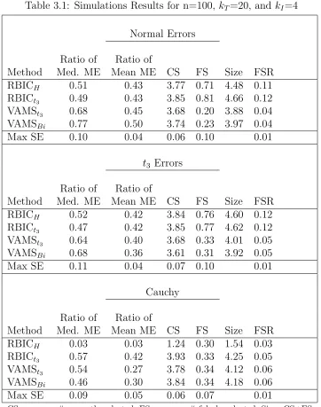
Table 3.1 Simulations Results for n=100, kT=20, and kI=4 . . . 60
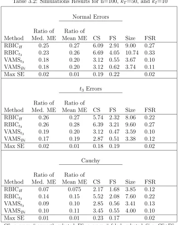
Table 3.2 Simulations Results for n=100, kT=50, and kI=10 . . . 61
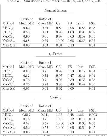
Table 3.3 Simulations Results for n=500, kT=50, and kI=10 . . . 62
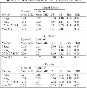
Table 4.1 Simulations Results for n=100, kT=20, and kI=4 . . . 72
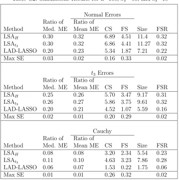
Table 4.2 Simulations Results for n=100, kT=50, and kI=10 . . . 73
Table 4.3 Simulations Results for n=500, kT=50, and kI=10 . . . 74
Table 5.1 Simulations Results for n=100, kT=20, and kI=4 . . . 79
Table 5.2 Simulations Results for n=100, kT=50, and kI=10 . . . 80
LIST OF FIGURES
Figure 2.1 Plot of response versus predictor . . . 21
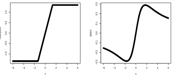
Figure 3.1ψ functions. Left panel: Huber ψ function, k=1; Right Panel: t3 ψ
function, v=3. . . 51
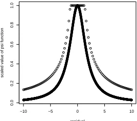
Figure 3.2 Huber and t3 M-estimation Weight functions. Huber: dotted line; t3:
Chapter 1
Robust Variable Selection
1.1
Introduction
Consider the linear model
Y =β01+Xβ+ǫ, (1.1)
whereY is a n×1 response vector, 1 is an×1 vector of ones,β0 is an intercept, X
is an n×kT design matrix,β is a kT ×1 vector of regression coefficients, and ǫis an
n×1 vector of independent and identically distributed errors. A statistical problem of interest is the determination of the relationship between the responseY and thekT
candidate predictors in the columns ofX. WhenkT is not very small, saykT >10, it
often makes sense to assume that only a fraction of the kT variables have coefficients
that are nonzero. We call those variables “informative” and use kI to denote the
number of such variables. The researcher is thus faced with two tasks, selecting the
informative candidate predictors and estimating their regression coefficients.
Two broad classes of variable selection procedures are subset selection methods and penalty methods. The class of subset selection methods includes procedures
such as forward selection, backward elimination, and stepwise regression. The class
on least squares methods that assume ǫ in (1.1) are normally distributed. The sen-sitivity of least squares to outlying points creates a need for robust alternatives to these standard variable selection procedures when errors come from a heavier tailed
distribution than the normal.
Although there are not many robust variable selection techniques, a variety of robust methods are available for estimating regression coefficients for a specified set
of predictor variables. Early robust procedures obtained estimates of the regression
parameters by replacing the squared error loss function with one that dampens the effects of outliers (Huber, 1973). More recent robust methods such as the least median
of squares (LMS), least trimmed squares (LTS), MM-estimation, and S-estimation
are focused on achieving high breakdown (introduced by Hampel, 1971; Donoho and Huber, 1983). None of these robust estimation procedures have built-in variable
selection capabilities.
We propose robust variable selection procedures that combine existing variable selection and robust regression procedures. Thus, in the remainder of this chapter
we give background information on subset selection and penalty methods as well
as on robust regression methods. In Chapter 2 we review the VAMS procedure, a
tuned version of forward selection that controls the false selection of unimportant predictors. Robust versions of the procedure are developed that allow for variable
selection and the elimination of potential outliers to occur simultaneously. With
outliers eliminated, the forward selection algorithm operates in a situation where it is known to perform well. In Chapter 3, existing robust regression procedures are
combined with variable selection. This requires the development of robust methods
for both obtaining and selecting from a group of candidate models. A new forward addition sequence based on the generalized score statistic (Boos, 1992) is introduced,
and a robust BIC is developed. Two LASSO-based robust variable selection methods
1.2
Model Selection Approaches
1.2.1
Subset Selection
Subset selection methods often follow a two-step process of obtaining a list of candidate models and using a selection criterion to determine which is optimal. One
possibility is to consider all subsets of the candidate predictors as potential
mod-els. For such an approach, the number of models, 2kT, increases exponentially with
the number of candidate predictors. While the all-inclusive nature of the approach
is appealing, the computational power needed for larger data sets is unreasonable.
Methods such as forward selection, backward elimination, and stepwise regression
are alternative procedures that provide a more manageable set of candidate models. Although these procedures can be viewed strictly as methods for obtaining candidate
models, the classical form of each is identified with a test-based stopping (or selection)
criteria. It is also common to select from the set of candidate models generated by each procedure using an information criteria.
Forward Selection
The forward selection algorithm generates candidate models by sequentially adding
predictors to the starting model containing just an intercept. At each step, a new
candidate model is formed by adding the predictor with the most significant one
de-gree of freedom F-test for entry into the model (most informative). Following this step-by-step process until all candidate predictors have entered the model leads to
a total of kT candidate models (in addition to the intercept-only model). Note that
the jth candidate model is composed of the first j variables in what we call the
for-ward addition sequence (FAS), a list specifying the order in which the kT candidate
predictors enter the model.
associ-ated with the F-statistic for entry is less than or equal to α. At the first step where the criteria is not met, the model building process stops and the current model is deemed optimal.
Backward Elimination
Similar to forward selection, the backward elimination procedure specifies kT
can-didate models. Starting from a full model containing allkT candidate predictors, the
algorithm generates candidate models by successively removing the predictor with the least significant one degree of freedom F-test for removal from the model (most
uninformative predictor). For this procedure the jth candidate model is composed
of all variables except the first j in the backward elimination sequence (BES), a list specifying the order in which the kT variables were removed from the model. The
requirement of a full model fit limits the use of the procedure to cases where the
number of candidate predictors is less than the sample size.
Much like forward selection, the standard backward elimination algorithm incor-porates a significance-based stopping criteria into the model building process using an
alpha-to-delete valueα. At each step, the least informative predictor is only removed from the model if thep-value associated with the F-statistic for removal is larger than
α. The final model is obtained when either no variables remain in the model or the criteria for removal is not met.
Stepwise Regression
The stepwise regression method combines the forward selection and backward
elimination algorithms. The method builds a model from one that contains just an
intercept. With an empty model the procedure starts like forward selection, with the addition of the most informative candidate predictor. However, unlike forward
selection, in each step the procedure is capable of removing predictors no longer
predictors. The predictors that are currently in the model are tested for removal
while the omitted variables are tested for inclusion.
Following the notation of forward selection and backward elimination, consider
using an alpha-to-enter value αin as a criteria for inclusion and an alpha-to-delete
value αout as a criteria for removal. After each step that a candidate predictor is
added to the model, all variables previously in the model are tested for removal. The
process continues until no variables meet the criteria to either enter or be removed
from the model. Note that unlike both the forward selection and backward elimination algorithms, a single list of candidate models for stepwise regression is not obtainable.
The list depends on the values αin and αout.
Information Criteria
Information criteria are often used to select from a set of candidate models. The
general form of an information criteria is
−2 logL(βb0,β,b bσ,Y) +q(p, n), (1.2)
where L(βb0,β,b σ,b Y) is a likelihood function evaluated at the maximum likelihood
estimates of the parameters and q(p, n) is a penalty for model complexity with p
equal to the dimension of (βb0,βb). Typical choices include the Bayesian information
criterion (BIC) with q(p, n) = plogn (Schwarz, 1978), Akaike information criterion (AIC) with q(p, n) = 2p, and Mallow’s Cp (Mallows, 1973), which is approximately
equal to the AIC. The common definition of each is developed assuming (1.1) is a Gaussian linear model. The first step to determining an optimal model is to calculate
the chosen information criterion for all candidate models. For either forward selection
or backward elimination this includes all models represented by the forward addition or backward elimination sequences. The model with the minimum value for the
information criteria is then declared optimal. There are other approaches to choosing
1993; Zhang, 1993).
1.2.2
Penalty Methods
Penalty-based variable selection methods obtain a model by solving a penalized
version of the least squares problem
b
β = arg min
( n
X
i=1
(Yi−xTiβ)2+p(λ,β)
)
. (1.3)
where xTi is the ith row of the design matrix X, p(.) is a specified penalty function,
and λ is a set of regularization parameters. Note that the Y and X variables are centered to have mean zero and that the columns ofX are scaled to have a variance of one. Thus, βb0 = ¯Y does not appear in (1.3). The penalty function shrinks the regression coefficients of certain variables to zero, leaving a model that contains only a subset of the original predictors. Common penalty methods include the LASSO
(Tibshirani, 1996), adaptive LASSO (Zou, 2006), and SCAD (Fan and Li, 2001)
pro-cedures. Specific technical details for the LASSO and adaptive LASSO are presented in Chapter 4, with robust alternatives to the procedure.
1.3
Robust Regression
1.3.1
M-estimation in Regression
Again consider the classical linear model (1.1) withǫcoming from a normal distri-bution with mean zero. Under these assumptions, the optimal method of estimating
regression coefficients is the method of least squares. However, many real data sets contain outlying observations that violate these assumptions. The method of least
squares is not optimal for outlier contaminated data sets, failing to provide stable
Consider the problem of obtaining regression coefficients that minimize some
func-tion ρ(.) of the residuals (Huber, 1973),
b
β= arg min
n
X
i=1
ρ[Yi−(β0+xTi β)]. (1.4)
Differentiating (1.4) with respect to β and setting the result equal to zero yields the estimating equations
n
X
i=1
ψ[Yi−(β0+xTi β)]
1
xi
!
=0, (1.5)
where ψ is the derivative of ρ. For a general ψ function, the regression coefficients that solve (1.5) are not invariant to changes in the scale of the dependent variable,
Y. For this reason, coefficients are obtained using
n
X
i=1
ψ
Yi−(β0+xTi β)
b
σ
1
xi
!
=0, (1.6)
wherebσis an estimate of scale used to standardize the residuals. Appropriate methods exist for estimating the scale parameter both prior to and simultaneously with the
regression coefficients. In either case an iterative algorithm is generally required to
solve (1.6). The final M-estimates of the regression coefficients are approximately normally distributed
b
β ∼N(β, ν(XTX)−1) (1.7)
with
ν =σ2 Eψ(u/σ)
2
[Eψ′(u/σ)]2, (1.8)
whereu follows the distribution of the regression erros andψ′ is the derivative of the
ψ function. The choice of the ψ function and the method of estimating σb determine the characteristics of the final M-estimates that solve (1.6). Research has shown that choosing a bounded ψ function, or even one that redescends to zero, leads to estimated regression coefficients that are robust to outlying observations. In Chapter
1.3.2
High Breakdown Methods
Hampel (1971, 1974) introduced the concept of breakdown and gross error
sen-sitivity as measures of robustness. A finite sample version of breakdown was later developed by Donoho and Huber (1983). The finite sample breakdown point is
de-fined to be the largest percentage of outlying points a sample can contain without
completely ruining the estimate of interest. Define the maximum bias of an estimator
T to be
b(ǫ;X, T) = sup|T(X(c))−T(X)| (1.9) where X is the original sample, X(c) is the contaminated sample, and ǫ is the per-centage of contamination. In (1.9) the supremum is taken over all ǫ-contaminated samples X(c). As defined by (Donoho and Huber, 1983) the breakdown point of the estimator T is then
ǫ∗(X, T) = inf{ǫ|b(ǫ;X, T) = ∞}. (1.10) Note that definition (1.10) is for estimators that are unbounded. In practice ǫ∗ is
often found by observing the minimum percentage of contamination that causes an
estimator to take on an arbitrarily large value. For bounded estimators it is equivalent to finding the percentage of contaminated data that will force an estimator to the
boundary of the parameter space (Donoho and Huber, 1983).
Consider two simple estimators of location, the mean and the median. Since a single large observation can cause the mean to become arbitrarily large, the statistic
has a breakdown point of 0. The median on the other hand has a breakdown point
of .5 since half the observations must be contaminated before the statistic fails to provide meaningful information about the original sample (Andrews et al., 1972).
Note that a breakdown point of .5 is the largest possible since for any higher level of
In a regression setting, a method that has good breakdown properties is able to
give meaningful estimates of the regression coefficients for highly contaminated data sets. Contamination can be in the form of outlying points in either the response or
independent variables. In this section we present three high breakdown regression
methods that are used throughout the rest of the thesis: the LMS, LTS, and MM-estimation procedures.
LMS and LTS procedure
The traditional least squares estimate is the one that minimizes the sum of squares
of the residuals. As discussed in section (1.1), the first robust alternatives to the least
squares method modified the basic procedure by replacing the square function by
something else. The most obvious example is the L1 estimate that replaces the square with the absolute value, and minimizes the sum of the absolute residuals. Rousseeuw
(1984) takes a different approach and instead replaces the sum with the median to
get
min
β med {r1(β)
2, ..., r
n(β)2}, (1.11)
where ri(β) = [Yi −(β0 +xTi β)] is the residual for the ith observation. The solution
to (1.11) is the Least Median of Squares (LMS) estimate. Rousseeuw (1984) shows
that the LMS estimate that solves (1.11) is both guaranteed to exist and obtains the
optimal breakdown point of fifty percent. A drawback of the LMS procedure is that the estimates have low efficiency.
Efficiency of estimates is not too important when the estimates are used as a
starting point for an iterative procedure. For this reason, Simpson et al. (1992) and
Rousseeuw (1984) use the LMS procedure to obtain preliminary estimates for their one-step M-estimators. Yohai (1987) takes a similar approach when constructing
MM-estimates. We follow these authors and use the LMS procedure strictly to generate
The low efficiency of the LMS procedure led Rousseeuw (1984) to develop the
least trimmed squares estimator (LTS) obtained by
min
β
h
X
i=1
r2i:n(β), (1.12)
where r2
1:n(β) ≤ r22:n(β). . . ≤ r2n:n(β) are the ordered squared regression residuals.
With an appropriate choice of h, the βb achieving the minimum in (1.12) is a high breakdown regression estimate that also has high efficiency.
MM-estimation
Like the LTS procedure of the last section, MM-estimation gives regression es-timates that not only have high breakdown but also high efficiency at the normal
distribution. Estimates are a modification of the typical M-estimates and are
ob-tained through a three-step process (Maronna, 2006, p. 125):
1. An initial consistent estimate βb(0) is computed that has high breakdown but not necessarily high efficiency. For example,βb(0) =βb(0)LM S, the least median of squares estimate. Although βb(0)LM S is inefficient it has the optimal breakdown point of .5.
2. A robust scale estimatebσis computed from the residuals of the high breakdown fit of the previous step. Using the residuals from the LMS fit, the robust
estimate of scale, σb, is found that solves the M-estimating equations
1
n
n
X
i=1
ρ ri
1.56σb
=.5. (1.13)
Hereri is theith residual from the LMS fit, and the constant 1.56 is chosen to
ρB(x) = min
1,1−(1−x2)3 . (1.14)
Like the initial estimate of the regression coefficients βb(0), the scale estimate obtained from (1.13) has a breakdown point of .5 (Maronna, 2006, p. 125).
3. The final MM estimateβb is found using an iterative procedure with βb(0) as a starting point. Using the estimate of scale found in the previous step the final
MM-estimates are found by solving
b
β = arg min
n
X
i=1
ρ
ri(β)
cbσ
, (1.15)
where ρ(.) is again the bi-square function and the scaling constant c is now chosen to have a desired efficiency at the normal distribution. Maronna (2006,
p. 30) presents a table showing the values of c for typical target levels of effi-ciency. For example, c=4.68 yields 95% efficiency at the normal distribution. The only restriction on c is that it is larger than 1.56, a requirement that is met for all reasonable efficiency levels.
As discussed in Section 1.3.1, solving (1.15) requires the use of an iterative
pro-cedure. Maronna (2006, p. 125) suggests the use of an iteratively re-weighted least
squares algorithm. For details of this procedure see Section 3.1. The final MM-estimates output by the iterative procedure are guaranteed to not have a breakdown
Chapter 2
Variable Addition Model Selection
In this chapter the variable addition model selection (VAMS) procedure is mod-ified to handle outlying points. Sections 2.1 and 2.2 outline the variable selection
problem and introduce the non-robust versions of the procedure. Then we introduce
the use of indicator variables and develop robust versions of the VAMS procedure that simultaneously select variables and eliminate outliers. Finally, Monte Carlo
sim-ulation is used to examine and compare the robust methods.
2.1
Simulation-Based VAMS
Using (1.1) as a starting point, the goal of a variable selection procedure is to determine which of the kT explanatory variables are informative. An informative
variable is defined as a variable having an associatedβithat is nonzero, while variables
with coefficients equal to zero are deemed uninformative. Ideally, when presented with a matrix of potential predictors, a variable selection procedure would choose a model
containing only informative variables. However, it is not possible for the variable
selection procedure to make this selection precisely, resulting in a model that is either over-fit or under-fit. A method is characterized as over-fitting if it tends to select
a significant number of uninformative variables along with the informative variables
predictors along with the failure to select informative variables with small but positive
regression coefficients. For a given data set (Y,X), the tendency of a particular method to over-fit or under-fit is related to the false selection rate (FSR), defined to
be
γ0 =E
U(Y,X)
1 +I(Y,X) +U(Y,X)
, (2.1)
where U(Y,X) and I(Y,X) are the number of selected uninformative and infor-mative predictors, respectively. The expectation in (2.1) is taken with respect to
repeated sampling of the data. With the addition of 1 in the denominator for the intercept, (2.1) is the expected proportion of uninformative predictors in the model.
Consider the case when data are entered into a variable selection procedure such as
forward selection. Depending on the alpha-to-enter tuning parameterα, the forward selection procedure selects models of differing size. In fact, the number of variables
selected is monotone in the tuning parameter α. As α increases from 0 to 1, the model grows from a model containing just an intercept to one that contains every predictor in the design matrix.
For a specific data set (Y,X), let S(α) be the total number of variables se-lected when applying the forward selection algorithm with a tuning parameter of α. Similarly, define U(α) and I(α) to be the number of uninformative and informative variables, respectively, in the selected model. The VAMS procedure introduced by
Wu et al. (2007) tunes the forward selection algorithm by providing an estimate of
α that attempts to keep the average false selection approximately equal to a target valueγ0.
Theoretically, this balance could be accomplished by estimatingαin the following way:
b
α = sup
α {
α:bγ(α)≤γ0}, (2.2)
wherebγ(α) is a function that estimates (2.1). By taking the supremum we obtain the largest possible model while keeping the FSR below the target rate γ0. If U(α) were
known, a natural choice for bγ(α) would be the empirical estimator U(α)/{1 +I(α) +
the empirical estimator with a suitable estimate.
The VAMS procedure estimates U(α) by monitoring the selection of user-created pseudo variables. These pseudo variables are uninformative variables generated so
that two key assumptions are satisfied approximately. The first is that the true
unimportant variables and the pseudo unimportant variables have on average the same probability of selection. The second is that the inclusion of the pseudo
vari-ables does not change the probability that an informative variable is chosen by the
variable selection procedure. Wu et al. (2007) proposed the following pseudo variable generation procedure.
Let Xp be the matrix formed by randomly permuting the rows of the design
matrix X. Then a matrix Z, whose kT columns consist of pseudo variables, can be
formed using the formula
Z = (I −P X)Xp. (2.3)
Here, I is an×n identity matrix andP X is the projection matrixX(XTX)−1XT.
Theith pseudo variable is then just the residuals from the regression of theithcolumn
ofXp on the predictors contained inX. The orthogonality of residuals to regressors,
inherent in linear regression, guarantees that the pseudo variables have a sample correlation of zero with the original predictors.
After creation of the pseudo variables, the matrix Z is appended to the original design matrixX, resulting in the augmented design matrixXV =X :Z of dimension
n×2kT. The forward selection algorithm is then applied to the new data set (Y,XV).
LetUp(α) be the number of pseudo variables selected when using a tuning parameter
of α. This process of generating pseudo variables and monitoring their selection is replicated for different permutations of the design matrixX. Then, for a fixedα, the rate θ at which the pseudo variables enter the model is estimated as
b
θ(α) = B
−1PB
i=1Up(α)
kT
= Up(α)
kT
, (2.4)
where B is the number of Monte Carlo replicates of pseudo variable generation and
assumption that the real unimportant variables and pseudo unimportant variables
have the same probability of being selected allows us to use (2.4) as an estimate of the rate at which the true unimportant variables are entering the model. Multiplying
this rate by an estimate of the number of uninformative candidate predictors
b
ku(α) = kT −S(α), (2.5)
results in an estimate ofU(α),{kT −S(α)}bθ(α). In (2.5), S(α) estimates the number
of candidate predictors in X that are informative.
Using the estimate of U(α), we can obtain the false selection rate estimate
b
γ(α) = {kT −S(α)}θb(α)
1 +S(α) . (2.6)
Substituting (2.6) into (2.2), results in an estimated α given by
b
α= sup
α≤αm
{α:bγ(α)≤γ0}, (2.7)
whereαmrestricts the search forαto be less than a predetermined maximum possible
value (generally .3). Using (2.7) as the tuning parameter for forward selection with the original data set (Y,X) leads to a selection procedure that controls the false selection rate. In practice, bγ(α) is calculated for a finite grid of α values, and the supremum in (2.7) is replaced by a maximum. By taking a fine enough grid there is little effect of the grid on the estimate of α.
2.2
Fast VAMS
After development of the standard VAMS procedure in the previous section, Boos
et al. (2008) proposed the simplified Fast VAMS procedure. Rather than estimating
the rate at which uninformative variables enter the model using (2.4), the new proce-dure sets bθ(α) equal to α. The Fast VAMS procedure therefore does not require the use of simulation. The new estimate of the FSR is then
b
γF(α) = {
kT −S(α)}α
which leads to
b
αF = sup α≤αm
{α:bγF(α)≤γ0}. (2.9)
Like the simulation version of the procedure, the final model is obtained using αbF as
the tuning parameter for forward selection with the original data (Y,X).
Boos et al. (2008) show that this is equivalent to selecting the model with size
k(γ0) = max{i: ˜pi ≤
γ0[1 +i]
kT −i
and ˜pi ≤αm} (2.10)
where ˜pis the sequence of monotonized p-values, that is,
˜
pi = maxpk fork = 1, ..., i. (2.11)
In (2.11), pk is the p-value to enter for the kth variable in the forward addition
sequence. An advantage of using (2.10) is that it does not require the computation
of αbF, that is, the final model can be obtained from examination of the sequential
p-values of the variables in the forward addition sequence.
Simulation results show that in addition to the large reduction in computation,
the Fast VAMS procedure leads to results comparable to the ones obtained from the simulation-based approach.
2.3
Simultaneous Selection and Outlier Detection
Mickey et al. (1967) described a modified approach to regression for detecting
outliers. Let X∗ =X :I where I is an n×n identity matrix. For the moment, we assume that the n×kT design matrix X is pre-specified and contains all regression
variables of interest. Then, stepwise regression is run using X∗ with all of the X
variables already included in the model. For an indicator variable, say thejthcolumn
ofI, we shall see that the test for entry into the model is identical to a significance test on the jth PRESS residual and that inclusion in the model is equivalent to deleting
the jth observation from the data set. Thus, Mickey et al. (1967) proposed a simple
Consider adding the jth column of the identity matrix, denotedI
j, to the
regres-sion of Y on the predictors in the design matrix X. The resulting regression model is
E(Y) =β01+Xβ+Ijδj, (2.12)
where β0, β, and δj are the regression coefficients for the intercept, X, and the
indicator variable Ij, respectively. The standard n− kT −2 degree of freedom t
-statistic
tn−kT−2(δj) =
b
δj
SE(bδj)
, (2.13)
tests the hypothesis H0 : δj = 0vs Ha : δj 6= 0, and measures the importance of
including Ij in the model. In (2.13), bδj is the least squares estimate of the regression
coefficient for Ij, and SE(bδj) is the standard error of this estimate. Since Ij is a
variable which affects only a single observation, bδj is the value that causes the jth
residual to obtain its minimum at zero. That is,
b
δj ={Yj −(βb0+xTjβb)}, (2.14)
wherexT
j is thejth row of X, andβb0 and βb are the least squares estimates ofβ0 and
β when Y is regressed on the predictors in X and the indicator variable Ij. Note
that with thejth residual necessarily equal to zero,βb
0 andβb are found by minimizing
the sum of squares of the remaining n−1 residuals. That is
(βb0,βb) = arg min n
X
i=1,i6=j
{Yi−(β0+xTi β)}2. (2.15)
In terms of estimation, the coefficients obtained using (2.15) are the same as those
obtained from the least squares regression ofY onXwith thejthobservation removed
from the data set. Returning to (2.14), we see thatδbj is then actually thejth PRESS
residual, a common outlier diagnostic, equal to the jth response minus the predicted
response for xT
j when thejth observation is excluded from the data set. An alternate
formula for calculating the jth PRESS residual using just the full data set is
P RESSj =
rj
1−Pxjj
where rj is the jth least squares residual and Pxjj is jth diagonal element of the
projection matrix Px =X(XTX)−1XT. An advantage of using (2.16) is that all n
PRESS residuals can be calculated using just a single least squares fit.
Since the stepwise regression procedure uses (2.13) to determine which indicators
enter the model, the final set of indicators are those with the most significant PRESS residuals. These indicators are therefore associated with the most outlying or
in-fluential observations. It is easy to show that for a model containing v indicators, (2.15) extends to obtaining regression coefficients (βb0,βb) that minimizen−v squared
residuals. Therefore, final regression coefficients are calculated with the observations
associated with the set of selected indicators removed from the data set.
To move from regression with outlier detection to variable selection with outlier detection, consider running the forward selection procedure with the augmented
de-sign matrixX∗ =X :I, containing both potential predictors and indicator variables. At each step of the algorithm, a variable is added to the model if it most significantly reduces the error sum of squares. Selection of an indicator variable implies that the
greatest reduction in the error sum of squares is obtained through removal of a single
observation. As in the fixed regression case, only indicator variables associated with
influential or outlying observations are likely to be selected. In terms of the potential predictors contained in X, the amount a variable reduces the error sum of squares is directly related to the level in which its regression coefficient significantly differs
from zero. This equivalence relationship implies that the variables selected from X
will be the ones that are deemed most informative by the data. Thus, the forward
selection algorithm sequentially selects potentially informative predictors and
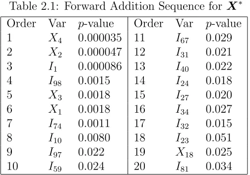
elimi-nates outliers by including columns of the identity matrix. As an example, in Table 2.1 we list the first twenty variables of the forward addition sequence for X∗.
Note that Mickey et al. (1967) did not suggest the use of stepwise regression
on both the indicators and original variables. Their stepwise search was just for the indicator variables, and thus merely a search for outliers in a fixed regression
Table 2.1: Forward Addition Sequence for X∗
Order Var p-value Order Var p-value
1 X4 0.000035 11 I67 0.029
2 X2 0.000047 12 I31 0.021
3 I1 0.000086 13 I40 0.022
4 I98 0.0015 14 I24 0.018
5 X3 0.0018 15 I27 0.020
6 X1 0.0018 16 I34 0.027
7 I74 0.0011 17 I32 0.015
8 I10 0.0080 18 I23 0.051
9 I97 0.022 19 X18 0.025
10 I59 0.024 20 I81 0.034
a procedure that not only performs variable selection but does so while adjusting for outlying points. The inclusion of indicator variables in the early steps of the selection
process means that variables are being considered for entry into the model with
multiple outlying points eliminated. If the eliminated outlying points are influential, their removal could significantly change the order in which the remaining variables
enter the model.
As with any application of forward selection, we are faced with the choice of an appropriate stopping criteria. By incorporating the indicator variables into either
the original simulation-based VAMS procedure (Section 2.1) or fast VAMS procedure
(Section 2.2), we can obtain an estimated alpha-to-enter valueαbthat controls the false selection of the original predictors in X. In this section we focus on the simulation-based indicator approach, a procedure we call VAMSI, but note that all the quantities
needed to use the fast VAMS procedure are also present.
Recall the key quantity to estimate is
b
γ(α) = {kT −S(α)}θb(α)
1 +S(α) . (2.17)
Here the value ofkT in (2.17) remains unchanged, still equaling the number of
be the number of original predictors selected, however it is now the result of applying
the forward selection algorithm to the data (Y,X∗ = X : I) instead of to (Y,X). In effect, we just ignore the selection of any indicators. As an example, consider the
forward addition sequence for X∗ presented in Table 2.1. If we assumeα =.02, the forward selection algorithm would choose a model containing the first eight variables in the sequence (I97is first variable with ap-value to enter greater thanα=.02). Since
only four of the eight are non-indicator variables coming from X, S(.02) = 4. Note, while indicators are ignored when calculating S(α), their inclusion in the forward selection process adjusts the selection of the variables in X (and hence the value of
S(α)) for the possibility of outliers.
The next step is to estimate the rate bθ(α) at which the uninformative predictors are entering the model. This rate is again estimated by monitoring the selection of
user created pseudo variables. LetXV I be the matrix formed by appending ann×n
identity matrix to the original VAMS design matrix XV, that is,
XV I = (XV :I) = (X :Z :I). (2.18)
The psuedo random variables in Z are generated using (2.3) and the original design matrix X. It should be noted that the design matrix in (2.18) contains 2kT + n
candidate predictors. Since the forward selection algorithm sequentially builds from a model including only an intercept, having more predictors than observations does
not pose a problem. However, if this procedure were to be extended to a variable
selection algorithm that required a full model fit, such as backward selection, having
more predictors than cases would be problematic.
For a particular α and matrix Z, Up(α) is now the number of pseudo variables
selected (ignoring the selection of indicators and original variables) when applying
the forward selection algorithm to the data set (Y,XV I). The rate at which
uninfor-mative predictors enter the modelθb(α), is then estimated using (2.4). With indicator adjusted definitions of kT, S(α) and θb(α) we have all the quantities needed to use
VAMSI procedure not only controls the false selection rate of the candidate predictors
but eliminates potentially outlying points. This is advantageous since traditionally the two tasks have been treated separately.
2.4
Outlier Detection Problems for VAMSI
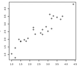
In this section we examine the merits of the VAMSI procedure as an outlier elim-ination method. In particular we find that a single αb cannot be used for selecting both original variables and indicators. Consider the simple linear regression data set
in Figure 2.1.
1.0 1.5 2.0 2.5 3.0 3.5 4.0 4.5
1.0
1.5
2.0
2.5
3.0
3.5
4.0
x
y
Figure 2.1: Plot of response versus predictor
This data set is one that is ideal for simple linear regression. There is a strong linear relationship between the response vector y and the single predictor x. With just a single predictor this is not a data set that is normally analyzed by a variable
selection procedure. However, we passed the data set to the VAMSI procedure to investigate the procedure’s ability to identify outlying observations. The VAMSI
procedure identified every observation as an outlier, an inappropriate result due to the
procedure fails to select an appropriate set of indicators when there is either very
few candidate predictors or all candidate predictors are strongly significant. First consider the case where there are very few candidate predictors. If indicators are
ignored, it is not uncommon to have two adjacent candidate predictors in the forward
addition sequence requiring drastically different estimates ofαto enter the model. For example, consider the variables X1 and X18 in Table 2.1. Ignoring indicators, these
two variables are adjacent in the forward addition sequence, butX1 enters the model
for any value ofαgreater than or equal to .0018 whileX18needs a value greater than or
equal to .051. Notice, for any value ofαbetween .0018 and .051, the forward selection algorithm chooses the same set of original predictors (X4, X2, X1, X3), making all
these models equivalent in terms of the VAMSI procedure. However, two different estimates within this gap can lead to a drastically different sets of indicators being
selected. Specifically, consider the models chosen by forward selection when using
α =.02 and α =.05. Withα =.02, four indicators are selected along with the four original predictors. For α =.05 the number of indicators selected grows to thirteen. A similar issue develops in the second case where all the candidate predictors are
highly significant. The VAMSI gives an inflated estimate of α to ensure that all the original predictors enter the model. Unfortunately, as we saw in the simple linear regression example, the inflated α can be large enough to also let in all the indicator variables.
To fix these problems we propose a dual estimation approach where tuning pa-rameter estimate αbX is used to select original variables and a separate estimate αbIND
is used to select indicators. Tuning the selection of the indicator variables should
result in a procedure with improved ability to properly identify outliers. In Section 2.4.1 we present three variations of the original VAMSI procedure. In Section 2.4.2 we
outline a two step approach that estimates the tuning parameters for the two types
2.4.1
Variations of VAMSI
All three methods presented in this section use the VAMSI procedure (Section 2.3)
to obtain αbX. Remember that this method uses the simulation-based estimate θb(α)
of the rate at which true unimportant variables enter the model to get an estimated
tuning parameter that controls of the false selection of the original predictors. Where
the methods differ is in their approach to obtaining αbIND, the tuning parameter for
the indicators. First we present the methods for obtaining αbIND and then show how
these estimates are combined with the αbX to select the final model.
V AM SI
1The VASMI1 procedure takes the simplest approach and obtains αbIND using the
simulation-free fast VAMS procedure. LetkIND be the number of observationsn, that
is, the number of indicator variables. Also, let SIND(α) be the number of indicators
that enter the model when applying the forward selection algorithm with a tuning parameter of α to the data (Y,X∗ = X : I). With kIND replacing kT and SIND(α)
replacing S(α) in (2.8), appropriate estimates of γ and α for the indicators are
b
γIND(α) =
{kIND−SIND(α)}α
1 +SIND(α)
= {n−SIND(α)}α
1 +SIND(α)
(2.19)
and
b
αIND = sup α≤αm
{α:bγIND ≤γ0} (2.20)
As with the previous VAMS methods αm is a restriction placed on the maximum
value ofα (generally equal to .3) and γ0 is the target false selection rate.
V AM SI
2The VAMSI2 method obtains an alternate fast VAMS estimateαbIND by replacing
SIND(α) in (2.19) with the simulation-based estimate of the number of informative
estimate θb(α), we calculate
SIND2(α) =
1
B
B
X
i=1
SINDP(α), (2.21)
whereB is again the number of Monte Carlo replicates of pseudo variable generation andSINDP(α) is the number of indicators selected when the forward selection algorithm
is applied to the data (Y,XV I = X : Z : I). Note that the value of SINDP(α) in
(2.21) differs from SIND(α) for the VASMI1 method. In that case, SIND(α) was the
number of indicators selected when the forward selection algorithm was applied to
the data set (Y,X∗ =X :I) containing no pseudo variables. Averaging across the bootstrap replicates to obtain (2.21) gives an estimate of the number of informative indicators that takes into account the variation across the different simulated data
sets. Also, since the calculation ofαbX already requires forward selection to be applied
to each simulated data set, the VAMSI2 procedure is computationally equivalent to
either the VAMSI or VASMI1 procedures.
Plugging (2.21) in to (2.19) gives
b
γIN D(α) = {
n−SIND2(α)}α
1 +SIND2(α)
, (2.22)
a new estimate of the false selection rate that can be used to calculate αbIND.
V AM SI
3Both the VASMI1 and VAMSI2 use some form of the fast VAMS procedure to
obtain an estimated forward selection entry criterion for the indicator variables. The VAMSI2 method used simulation to obtain an alternate estimate of the number of
informative indicators, butαbINDwas still found using (2.19) and (2.20). In this section
a procedure is developed that uses the simulation version of the VAMS procedure to obtain αbIND.
When dealing with the indicator variables the generation of pseudo variables is
pseudo variables are generated for the candidate predictors through permutation of
the design matrix X. When considering a matrix of indicators the permutation method is no longer appropriate. Random permutation of the rows ofI would result in a matrix containing the same set of variables. Wu et al. (2007) outlines alternative
approaches to pseudo variable generation. In one such approach, psuedo variables are generated by simply taking a random sample from a standard normal distribution. As
with the permutation-based method, the resulting pseudo variables are stochastically
uncorrelated with the true predictors (Wu et al., 2007).
Using the new approach, a matrix ZI consisting of n standard normal pseudo
variables is formed. For a chosen alpha, let Uz(α) be the number of these standard
normal pseudo variables selected when the forward selection algorithm is applied to the data (Y,[X :ZI : I]). Redefining (2.4), the rate which unimportant indicators
are entering the model can be estimated as
b
θIN D(α) =
B−1PB
i=1Uz(α)
n =
Uz(α)
n , (2.23)
leading to
b
γIND(α) =
{n−SIND(α)}θbIND(α)
1 +SIND(α)
. (2.24)
We now have all the quantities needed to obtain the VAMSI3 simulation-based
esti-mate αbIND for the indicator variables.
Determining the Final Model
Regardless of the method used to find αbIND, the final model is determined through
two separate applications of the forward selection algorithm to the data (Y,X∗ =
X : I). Specifically, the set of indicators are selected using a forward selection tuning parameter of αbIND, and the original predictors are selected using the tuning
parameter αbX. To illustrate this process with Table 2.1, suppose that for one of
the three procedures above αbX = .028 and αbIND = .001. The result of applying
variables X4, X2, I1, I98, X3, X1, I74, I10, I97 and I59. Thus the original predictors
(X4, X2, X3, X1) enter the final model. The second application of forward selection
with αbIND = .001 gives a model with just three variables X4, X2 and I1. Thus the
single indicatorI1 enters the model. The chosen method in this case therefore selects
a model consisting of the variables X4, X2, X3, X1 and I1. Note that since all three
methods in this section use the sameαbX estimate, they select the same set of original
predictors. However with different estimates ofαbIND, the set of indicators selected can
be different.
2.4.2
Two-Stage Methods
Another approach to obtaining estimatesαbIND and αbX for the indicators and
orig-inal predictors is to carry out the estimation in two stages. In the first stage an estimate of α for the indicators is obtained. Like the VASMI1 procedure we use the
fast VAMS estimates (2.19) and (2.20).
The estimated tuning parameter αbIND is used to perform forward selection on the
augmented data (Y,X∗). Although, the forward selection algorithm selects both original predictors and indicators, in the first stage we are only concerned about the
set of indicators selected. Returning to the sample forward addition sequence in Table 2.1, assume thatαbINDequals .025. Forward selection chooses a model consisting of the
first 10 variables in the sequence. Under these circumstances, the variables of interest
are the six indicators I1, I98, I74, I10, I97 and I59. The first stage concludes with
the elimination of the observations associated with the set of selected indicators. We
would then delete observations 1,98,74,10,97, and 59 from the data set. In general,
this leaves a regression data set with n−SIND(αbIND) observations.
With the outliers removed from the data set, a “clean” subset of the data remains.
There is no longer any need to use indicator variables. The least squares methods
inherent in the original VAMS procedures are now in a situation where they are known
data that remains. The αbX estimate obtained controls the false selection rate of the
original variables contained in X. To distinguish between the two types of two-stage methods, we will refer to the procedure that uses simulation in the second stage as
“TWO SIM.” The procedure that uses fast VAMS for the second stage will be called
“TWO FAST.” Using the two stage approach gives a robust procedure that controls the false selection rate of both the original predictors and the indicators variables.
2.4.3
Summary
In this section five dual estimation approaches were introduced VASMI1, VAMSI2,
VAMSI3, TWO SIM, and TWO FAST. Each of these procedures are designed to
ob-tain separate tuning parameter estimates for the original predictors and indicator
variables. With a common goal, it is not surprising that many of these procedures are only slight variations of one another. VASMI1, VAMSI2, and VAMSI3 all use the
same estimate ofαbX. In terms of estimating the tuning parameter for the indicators,
the TWO SIM, TWO FAST, and VASMI1 procedures all use exactly the same version
of the fast VAMS procedure. The VAMSI2 is then a slight variation of this approach,
using the fast VAMS procedure but with a modified estimate of the number of
in-formative indicators. With the TWO SIM and TWO FAST procedures declaring the same set of observations as outliers, the difference in the estimated tuning parameters
for the original predictors is directly attributable to differences in performance of the
original simulation and fast VAMS procedures. Previous simulation results suggest that this difference should be minimal. In the next section, Monte Carlo
simula-tion is used to further investigate the differences between these five variable selecsimula-tion
2.5
Comparison of Methods
2.5.1
Data Generation
To study the performance of the robust variable selection procedures presented thus far, we use Monte Carlo Simulation. Each of the one-hundred Monte Carlo
replicates of the variable selection process requires the generation of data from the
linear regression model (1.1). The data generation process presented here follows closely that of Luo et al. (2006).
Each row of then×kT design matrix X is generated from an AR(1) process with
parameter θ, giving the relationship
X[i, j] =θ(X[i, j −1]) +eij j = 2, ..., kT, (2.25)
with X[i,1] randomly generated from a standard normal distribution. In (2.25), the
eij are independent errors taken from a standard normal distribution leading to a
variance-covariance structure of the form
V(X[i, j]) = 1
1−θ2 (2.26)
Cov(X[i, j], X[i, j +l]) = 1 1−θ2θ
|l|. (2.27)
Scaling each row of the design matrix by the normalizing constant
cρ=
√
1−θ2 (2.28)
forces the variance ofX[i, j] to be one and the covariance betweenX[i, j] andX[i, j+l] to beθ|l|.
In an attempt to make the design matrix have a variety of predictor variables, a proportion of the columns are transformed. The first half of the predictor variables
are not transformed and keep their original values. The next one-fourth of the initial
predictors are chosen to be dichotomous variables. These columns are redefined so that the jth entry, x
j becomes x∗j where
x∗j =
(
1 when xj ≥0
0 when xj <0.
The last fourth of the predictors are transformed via the absolute value function.
Our final design matrix is obtained by centering, scaling, and randomly permuting the columns of the transformed matrix. The random permutation of the columns has
two benefits. It mixes up the original and transformed variables and avoids having
only adjacent variables with high correlation.
Through construction of our β vector, we specify the proportion of informative predictors. For all situations, one fifth of the kT predictor variables are chosen to be
informative and given initial regression coefficients equal to 1, while the remaining entries in the β vector are set to zero.
After the initial β vector is created, the coefficients of the informative predictors are scaled to control the strength of the linear relationship between Y and X. The variable selection procedures are more likely to identify informative variables when
the relationship between Y and X is strong. In the context of regression models, the coefficient of determination,R2, is commonly used to quantify the strength of the
linear relationship. The formula for theoreticalR2 with random predictors is
R2 = var(X
Tβ)
var(XTβ+ǫ). (2.30)
A drawback of using the standard version of R2 is that it requires the existence
of moments, a feature that eliminates error distributions such as the Cauchy from consideration. Also, since the variance is a non-robust measure of variability, using
(2.30) is not appropriate for data containing outlying points. Replacing the variance
with the square of the median absolute deviation (MAD), results in a less restrictive,
robust version of R2 defined to be
R2rob = {MAD(X
Tβ)
}2
{MAD(XTβ+ǫ)}2. (2.31)
Now the robust coefficient of determination can be used to control the strength of the
Using the scaled version of β along with the final design matrix X, we get the corresponding regression mean vectorµ using the relationship
µ=E(Y|X) =E(β01+XTβ+ǫ) =β0+XTβ. (2.32)
with the true intercept β0 set equal to one. The response vector Y is obtained via
Y =µ+ǫ. (2.33)
Here1is a vector with each entry equal to one, that specifies the value of the regression
models intercept and ǫ is a vector containing n independent identically distributed errors. When choosing the distribution of ǫ, one must consider the effect that the distribution has on the data and hence the variable selection procedures. For example,
errors sampled from a standard normal distribution result in data relatively free of outliers. However, choosing heavier tailed distributions like the t or Cauchy changes both the frequency and magnitude of the outlying points in the data set. Creating
simulation data sets using a variety of error distributions allows for insight into how outliers affect the variable selection procedures.
2.5.2
Simulation Design
In this section, we present the Monte Carlo Simulation design used to study the
performance of the VAMS procedures developed in this chapter. These procedures
include the non-robust version of the VAMS presented in Section 2.1, VAMS with
indicators (VAMSI), and all the dual estimation approaches with the exception of VAMSI3. In preliminary studies the VAMSI3 procedure proved to be computationally
intensive and performed no better than the other dual estimation methods.
Our design uses simulated data sets generated using the method described in Section 2.5.1, with an AR(1) parameter ofθ=.5 and a target R2
rob of .5. The number
of observations, number of candidate predictors, and the distribution of the regression
errors then follow a 2×2×3 design. Data sets are generated with eithern = 100 or
and kT = 50. Finally, the regression errors are generated from three distributions:
standard normal, t with three degrees of freedom, and Cauchy. For comparison purposes thet3 error distribution is scaled by the square root of the degrees of freedom
(three) to get a variance of one.
While the Cauchy distribution does not have a finite second moment, it is possible to select a scale parameter that will make the Cauchy distribution mimic a
standard-ized distribution in terms of the percentage of nonoutlying points. One way to do this
is to match up quantiles. We wanted the Cauchy distribution to mimic the standard normal so we chose the scale parameter that made 95 percent of the distributions
mass fall between −1.96 and 1.96. This amounts to solving
{s:Fc,s(1.96)−Fc,s(−1.96) =.95} (2.34)
where Fc,s is the Cauchy distribution function with a scale parameter of s. Solving
(2.34) gives a scale parameter of .154. While 95% of the mass for the scaled Cauchy
distribution is between −1.96 and 1.96 the heavy tail allows for the possibility of outlying points uncommon to the standard normal distribution. We thus have our three error distributions: standard normal, scaledtwith three degrees of freedom and Cauchy with a scale parameter of .154.
The performance of the VAMS procedures under these conditions is compared in terms of the following criteria:
•Ratio of Med. ME = median model error of “optimal” model divided by the median model error of selected models
• Ratio of Mean ME = mean model error of “optimal” model divided by the mean model error of selected models
• CS = average number of informative predictors selected
• FS = average number of uninformative predictors selected
• Outliers = average number of indicator variables selected
• Size = CS+FS= average number of original predictors selected
• αbX= average estimated α for the original predictors
• αbIND= average estimatedα for the indicator variables
For the Ratio of Median ME and Ratio of Mean ME, the model error for a single
data set is defined to be
ME = 1
n
n
X
i=1
(ybi−µi)2 (2.35)
where ybi is the ith predicted response and µi is the ith value in the mean vector
µ. For each data set a model error is also calculated for the “optimal” model. The optimal model is one consisting of all the informative predictors and no uninformative
predictors. The method of obtaining fitted values for this model depends on the
distribution of the errors. For normal distributed errors, least squares regression is used. For t3 and Cauchy errors, the method of maximum likelihood is used to obtain
estimated regression coefficients for each of the informative predictors.
2.5.3
Results
Tables 2.2-2.4 contain results for the VAMS procedures. There is a consistent
difference in the number of outliers selected by the procedures across each of the
sim-ulation conditions. First consider the case when the errors are normally distributed. Each of the dual estimation approaches are eliminating significantly fewer outliers
than the original VAMSI procedure. In Table 2.2, when n = 100 and kT = 20, the
number of selected outliers is 1.67 for VAMSI compared to .13 or less for the dual estimation methods. A drop in the number of declared outliers is also seen when the
errors come from the t3 distribution. However, when we move to Cauchy errors the
dual estimation methods start to select more outliers than the VAMSI procedure. Specifically, we see an increase from 15.04 outliers for the VAMSI procedure to 18
or more for the dual estimation approaches. By tuning the selection of the indicator
from a heavy tailed distribution.
In Table 2.2, we see that both of the model error ratios are similar across the five robust VAMS procedures. This is a result we expect, since many of these procedures
are only slight variations of one another. Remember that the VAMSI, VASMI1, and
VAMSI2 procedures all select original predictors by the same method. In spite of
this, the fact that the VASMI1 and VAMSI2 procedures select fewer outliers than
the VAMSI procedure leads to a slight improvement in terms of model error when
the errors are normally distributed. Staying with normal errors, the two-stage meth-ods have a slight edge in terms of selection characteristics. Both the TWO FAST
and TWO SIM procedures select on average more informative predictors and less
uninformatives than the other VAMS procedures. For t3 errors the relationship is
reversed. Now the two-stage methods are doing slightly worse than the other dual
estimation methods both in terms of model error and selection characteristics. With
the heavier-tailed errors t3 errors, we see a clear separation between the non-robust
and robust versions of the VAMS procedures. With Cauchy errors the effect is even
more pronounced. The original VAMS procedure selects on average more
uninfor-mative than inforuninfor-mative predictors. Another issue is the failure of the TWO SIM
procedure for Cauchy distributed errors. Upon further inspection the procedure fails if enough outliers are removed from the data set, in the first stage of the procedure,
to make the number of observations less than the number of predictors. With the
number of observations less than the number of predictors generation of (2.3), the matrix of pseudo variables, is impossible due to the singularity of XTX. Since the issue is with the generation of the pseudo variables, the TWO FAST procedure is
unaffected.
Another important criterion is the false selection rate. Each of these methods are
designed to obtain a false selection rate of .05. In Table 2.2 all five of the robust
methods do an excellent job, hitting the target on average for normally distributed errors. The procedures have a little more difficulty for the heavier tailed errors but
In Table 2.3 the conditions shift to n = 100 and kT = 50. These conditions are
much more difficult for the variable selection procedures to handle. For normally distributed errors, the procedures are selecting on average about forty percent of
the informative predictors compared to ninety-three percent under the previous set
of conditions. An even smaller proportion are selected for the heavier tailed error distributions. In terms of model error, the TWO FAST procedure does worse than
the other procedures. This is most evident when the errors have a Normal or t3
distribution. The procedure is fitting a significantly smaller model than the others. The TWO SIM procedure now fails for botht3 and Cauchy errors. The large number
of candidate predictors makes it easier for the number of observations to fall below the
number of candidate predictors. Compared to the results seen in Table 2.2, each of the dual estimation procedures are doing a poor job of keeping the false selection rate
near the target rate of .05. Even for normally distributed errors the false selection
rate is in the range of .12-.15.
For Table 2.4 the number of observations is raised to five hundred while kT
re-mains equal to fifty. With the number of observations being ten times the number of
candidate predictors the variable selection procedures do a good job of distinguishing
between the informative and uninformative predictors. The four dual estimation ap-proaches have comparable model error ratios for all error distributions, with a slight
edge going to the VAMSI2 procedure. For Normal errors the VAMSI procedure does
worse than the competition in terms of model error. Again this can be attributed to the procedure not tuning the selection of the indicator variables. With the increase
in the number of observations, the false selection rates are again close to their target
value of .05. Only for the Cauchy errors are they slightly inflated to around .08. The similarity of results to those seen in Table 2.2 suggests that the abnormalities
exhibited under the second set of conditions were not simply due to an increase in the
number of candidate predictors but the relationship between the number of candidate predictors and the number of observations. When the number of observations is large
do a good job of both separating the informative and noninformative predictors and