Variational Modeling and Complex Fluids

Mi-Ho Giga, Arkadz Kirshtein, and Chun Liu

Abstract

In this chapter, a general energetic variational framework for modeling the dynamics of complex fluids is introduced. The approach reveals and focuses on the couplings and competitions between different mechanisms involved for specific materials, including energetic contributions vs. kinematic transport relations, conservative parts vs. dissipative parts and kinetic parts vs. free energy parts of the systems, macroscopic deformation or flows vs. microscopic deformations, bulk effects vs. boundary conditions, etc. One has to notice that these variational approaches are motivated by the seminal works of Rayleigh (Proc Lond Math Soc 1(1):357–368, 1871) and Onsager (Phys Rev 37(4):405, 1931; Phys Rev 38(12):2265, 1931). In this chapter, the underlying physical principles and background, as well as the limitations of these approaches, are demonstrated. Besides the classical models for ideal fluids and elastic solids, these approaches are employed for models of viscoelastic fluids, diffusion, and mixtures.

Contents

1 Introduction. . . 2

2 Nonequilibrium Thermodynamics. . . 4

2.1 Energetic Variational Approaches. . . 4

2.2 Hookean Spring. . . 7

2.3 Gradient Flow (Dynamics of Fastest Descent). . . 8

3 Basic Mechanics. . . 10

3.1 Flow Map and Deformation Gradient. . . 10

3.2 Newtonian Fluids and Navier-Stokes Equations. . . 12

M.-H. Giga

Graduate School of Mathematical Sciences, University of Tokyo, Tokyo, Japan e-mail:[email protected]

A. Kirshtein () • C. Liu

Department of Mathematics, Pennsylvania State University, University Park, PA, USA e-mail:[email protected]; [email protected]

© Springer International Publishing AG 2017

Y. Giga, A. Novotny (eds.), Handbook of Mathematical Analysis in Mechanics of Viscous Fluids, DOI 10.1007/978-3-319-10151-4_2-1

3.3 Elasticity and Viscoelasticity. . . 14

3.4 Other Approaches to Elastic Fluids. . . 17

3.5 Generalized Diffusions. . . 21

4 Complex Fluid Mixtures: Diffusive Interface Models. . . 25

4.1 Surface Tension and the Sharp Interface Formulation. . . 25

4.2 Diffusive Interface Approximations (Phase Field Methods). . . 27

4.3 Boundary Conditions in the Diffusive Interface Models. . . 33

5 Conclusion. . . 34

Cross-References. . . 36

References. . . 36

1

Introduction

The focus of this chapter is on the mathematical modeling of anisotropic complex fluids whose motion is complicated by the existence of mesoscales or subdomain structures and interactions. These complex fluids are ubiquitous in daily life, includ-ing wide varieties of mixtures, polymeric solutions, colloidal dispersions, biofluids, electro-rheological fluids, ionic fluids, liquid crystals, and liquid-crystalline poly-mers. On the other hand, such materials often have great practical utility since the microstructure can be manipulated by external field or forces in order to produce useful mechanical, optical, or thermal properties. An important way of utilizing complex fluids is through composites of different materials. By blending two or more different components together, one may derive novel or enhanced properties from the composite. The properties of composites may be tuned to suit a particular application by varying the composition, concentration, and, in many situations, the phase morphology. One such composite is polymer blends [121]. Under optimal processing conditions, the dispersed phase is stretched into a fibrillar morphology. Upon solidification, the long fibers act as reinforcement and impart great strength to the composite. The effect is particularly strong if the fibrillar phase is a liquid-crystalline polymer [99]. Another example is polymer-dispersed liquid crystals, with liquid crystal droplets embedded in a polymer matrix, which have shown great potential in electro-optical applications [127].

elastic effects can be represented in terms of certain internal variables, for example, the orientational order parameter in liquid crystals (related to their microstructures), the distribution density function in the dumbbell model for polymeric materials, the magnetic field in magnetohydrodynamic fluids, the volume fraction in mixture of different materials, etc. The different rheological and hydrodynamic properties will be attributed to the special coupling (interaction) between the transport (macroscopic fluid motions) of the internal variable and the induced (microscopic) elastic stress [115,116]. This coupling gives not only the complicated rheological phenomena but also formidable challenges in analysis and numerical simulations of the materials.

The common feature of the systems described in this chapter is the underlying energetic variational structure. For an isothermal closed system, the combination of the first and second laws of thermodynamics yields the following energy dissipation law [6,11,39,56]:

d dtE

total_{D ; (1)}

whereEtotal_{is the sum of kinetic energy and the total Helmholtz free energy and} is the entropy production (here the rate of energy dissipation). The choices of the total energy functional and the dissipation functional, together with the kinematic (transport) relations of the variables employed in the system, determine all the physical and mechanical considerations and assumptions for the problem.

The energetic variational approaches are motivated by the seminal work of Rayleigh [106] and Onsager [100,101]. The framework, including Least Action Principle and Maximum Dissipation Principle, provides a unique, well-defined, way to derive the coupled dynamical systems from the total energy functionals and dissipation functions in the dissipation law (1) [67]. Instead of using the empirical constitutive equations, the force balance equations are derived. Specifically, the Least Action Principle (LAP) determines the Hamiltonian part of the system [2, 5,50], and the Maximum Dissipation Principle (MDP) accounts for the dissipative part [11,101]. Formally, LAP represents the fact that force multiplies distance is equal to the work, i.e., ıE D force ıx; where x is the location and ı the variation/derivative. This procedure gives the Hamiltonian part of the system and the conservative forces [2,5]. The MDP, by Onsager and Rayleigh [67,100,101,106], produces the dissipative forces of the system,ı1

2 D forceıx:P The factor 1 2 is consistent with the choice of quadratic form for the “rates” that describe the linear response theory for longtime near-equilibrium dynamics [74]. The final system is the result of the balance of all these forces (Newton’s Second Law).

2

Nonequilibrium Thermodynamics

In this section, some basic thermodynamic principles and general relations between energy laws and differential equations are described. We first clarify notation of variations of the functionals [50,54]. LetE D E. /be a functional depending on a function in a spaceH which is equipped with an inner producth; iH. The variationıE Dı Eof a functionEis defined as

ı E. /D lim

h!0ŒE. Chı /E. / =h;

whereı is a function so that Chı is a variation of . The quantityı E is often called a directional derivative in the direction ofı at . It is formally the Gâteau derivative ofEat in the direction ofı . Ifı Ecan be written as

ı E. /D hf; ı iH;

with somef for a big class ofı , we often writef by

H_ıE

ı or simply ıE ı :

This quantity corresponds to the total derivative or the Fréchet derivative if the latter is well defined [55]. It is simply called the variational derivative . In this notation, denominator points to the function with respect to which the variation of the functional in the numerator is taken.

2.1

Energetic Variational Approaches

The first law of thermodynamics [56] states that the rate of change of the sum of kinetic energyKand the internal energyU can be attributed to either the workWP done by the external environment or the heatQP:

d

dt.KCU/D PW C PQ:

In other words, the first law of thermodynamics is really the law of conservation of energy. It is noticed the internal energy describes all the interactions in the system. In order to analyze heat, one needs to introduce the entropyS[56], which naturally leads to the second law of thermodynamics [39,56]:

TdS

where T is the temperature and S is the entropy. is the entropy production which is always nonnegative and gives the rate of energy dissipation in irreversible systems. Subtracting the two laws, in the isothermal case whenT is constant, one arrives at:

d

dt.KCUTS/D PW ;

whereFDUTSis called the Helmholtz free energy. We denoteEtotal_DKCF to be total energy of the system. If the system is closed, when work done by the environmentWP D0, the energy dissipation law of the system can be written as

dEtotal

dt D 2D: (2)

The quantityDD 1₂is sometimes called the energy dissipation. The dissipative law allows one to distinguish two types of systems: conservative (or Hamiltonian) and dissipative.

The choices of the total energy components and the energy dissipation take into consideration all the physics of the system and determine the dynamics through the two distinct variational processes: Least Action Principle (LAP) and Maximum Dissipation Principle (MDP).

To derive the differential equation describing the conservative system (D 0), one employs the Least Action Principle (LAP) [2,5], which says that the dynamics is determined as a critical point of the action functional (Remark 1 below). We give its equivalent form. We consider functionalsR₀TKdt andR₀T Fdtdefined for a function x (the trajectory in Lagrangian coordinates, if applicable) depending on space time variables. The inertial and conservative force from the kinetic and free energies are, respectively, defined as

forceinertialDH_

ıR₀TKdt ıx ;

forceconservativeDH_

ıR₀TFdt ıx :

The spaceH is typically taken as the space timeL2 _{space, L}2

x;t, i.e., L2x;t D L2_{.0; TIL}2

x/, whereL2xis theL2 space in the spatial variables. (These are called variational forces.) In other words, for allıx,

ı Z T

0

KdtD hforceinertial; ıxiL2 x;t D

Z T

0

hforceinertial; ıxiL2 xdt

ı Z T

0

FdtD hforceconservative; ıxiL2x;t D

Z T

0

The LAP can be written as

ı Z T

0

KdtDı

Z T

0

Fdt

for allıx. This gives the natural variational form (the weak form) of the forces with

suitable test functionsıx. The strong form of the system (Euler-Lagrange equation)

can be also written as a force balance (without dissipation).

forceinertialDforceconservative: (3)

The inertial force corresponds to the inertial termmain Newton’s Second Law, whereais the acceleration andmis the mass. Note that if the variation is performed on a bounded domain and involves integration by parts, one has to assume specific boundary conditions to cancel the boundary terms, so that no boundary effects are involved.

Remark 1. The standard approach [5] dictates to define the Lagrangian functional

L D KF and the action functional as A.x/ D R₀TLdt. The Euler-Lagrange equation in this case isH_ı_ıxAD0.

For a dissipative system .D2D> 0/, according to Onsager [100,101], the dissipationDis taken to be proportional to a “rate” xt raised to a second power. The Maximum Dissipation Principle (MDP) [67] implies that the dissipative force may be obtained by minimization of the dissipation functionalDwith respect to the above mentioned “rate.” Hence, through MDP, the dissipative force (linear with respect to the same rate function) can be derived as follows:

ıDD hforcedissipative; ıxti_HQ:

In other words,

Q

H_ıD=ıxt Dforcedissipative:

Note that the test function in MDP is different from that in LAP before.

Remark 2. It is important to note that although the limitation for the dissipationD

to be quadratic in “rate” is rather restrictive, strong nonlinearities can be introduced through coefficients independent of the “rate.”

When all forces are derived, according to the force balance (Newton’s Second Law, where inertial force plays role ofma):

Notation. For shorter notation, one can write Eq. (4) as H_ı

RT 0 Kdt

ıx D

H_ı

RT 0 Fdt

ıx C QH_ ıD

ıxt withHDL

2_{.0; TI QH /.}

It is important to notice that Eq. (4) uses the strong form of the variational result. This might bring ambiguity in the original variational weak form, since the test functions may be in different spaces.

2.2

Hookean Spring

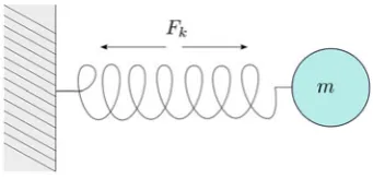
As a start, a simple ordinary differential equations (ODE) example of a dissipative system is considered here, which had been originally proposed by Lord Rayleigh [106]: the Hookean spring of which one end is attached to the wall and the other end to a mass m (see Fig.1). Let x .t / be a displacement of the mass from the equilibrium. Consider that the spring has friction-based damping which is proportional to the velocity (relative friction to the resting media). Under these assumptions,

KD mx

2 t

2 ; FD

kx2

2 ;and DD x2

t 2 ;

where k is spring strength material parameter and is damping coefficient. The energy dissipation law is clearly as follows:

d dt

_mx2 t

2 C

kx2 2

D x2 t:

The corresponding action functional of the spring [50] in terms of the position x.t /:

AD

Z T

0 _mx2

t

2

kx2 2

dt:

Then the Least Action Principle, i.e., variation with respect to the trajectoryx.t /, yields [50]:

ıAD Z T

0

Œmxt.ıx/_tkxıx dt D Z T

0

.mxt t kx/ ıx dt

D

L2_t_ıA ıx; ıx

L2_{.0;T /} D

Z T

0

L2_t_ıA ıx; ıx

R dt:

Here the spaceH with inner product isL2

t D L2.0; T /because hereL2xis just R. On the other hand, the principle of maximum dissipation gives

R_ıD ıxt D xt:

Indeed, looking at forces involved and formulating Newton’s Second Law (F D

ma) for this system, one can getmxt t D kx xt;or equivalently

mxt tC xtCkxD0; (5)

which is equivalent to the variational force balance (corresponding to (4))L2 t_ııxA D R_ı_ıxD

t for this example.

Looking at the explicit solution of (5), it is clear that the Hamiltonian part describes the transient dynamics, the oscillation near initial data, while the dissi-pative part gives the decaying longtime behavior near equilibrium.

2.3

Gradient Flow (Dynamics of Fastest Descent)

The energetic variational approaches have many different forms in practices and applications. Next look at the familiar example of gradient flow (dynamics of fastest descent):

ıF.'/

ı' C't D0; (6)

whereFis a general energy functional in terms of'. Here'is a function of spatial variables with parameter time t, and the constant > 0 is the dissipation rate which determines the evolution approaching the equilibrium. Such a system has been used in many applications both in physics and in mathematics; in particular, it is commonly used in both analysis and numerics to achieve the minimum of a given energy functional.

It is clear that with natural boundary conditions (Dirichlet or Neumann), the solution of (6) satisfies the following energy dissipation law (by chain rule and integration by parts, if needed):

d

dtF D

Z

1 j'tj

2 dx;

On the other hand, one can put this in the general framework of energetic variational approaches. Notice that there is no kinetic energy in this system, indicating the nature of being the longtime near-equilibrium dynamics.

Notation. When working on a bounded domain, one should consider a variation up to the boundary. Generally, for a functionalEdepending on a function defined in, the variationı Eis often of the form

ı E. /D Z

f ı dxC Z

@

gı dS:

Then, we denote

f D ıE

ı

; gD ıE

ı@ :

Heref gives variational force inside the domain, whilegis a kind of a boundary force. So if the boundary is taken into account, boundary forces should be also balanced.

Unless mentioned otherwise, in this chapter, specific boundary conditions are taken to cancel the boundary effects (i.e., make boundary integral equal to zero).

In the case ofF D RW .';rx'/ dx and D D ₂1 Rj'tj2_{dx, the variation} leads to the following two variational derivatives:

L2x_ ıF ı'

D r @W

@r' C @W

@' ; L 2 x_

ıD ı't

D 1

't;

which after substitution in (4) yield equation (6). In this case, the boundary effects would be canceled out in case of homogeneous Dirichlet or Neumann boundary conditions.

Remark 3. To derive implicit Euler’s time discretization scheme [8], one may

consider minimization of the following functional:

min

'nC1 given'n

Z

(

1 ˇ

ˇ'nC1'nˇˇ2

2t CW

'nC1;r'nC1 )

dx:

3

Basic Mechanics

Before moving on to more complicated and realistic applications, it is important first to introduce some basic terminologies and concepts in continuum mechanics [36,59]. In particular, in this section, the relation between Eulerian (space reference) and Lagrangian (material reference) coordinates [119] is explored, and the varia-tional techniques in terms of deformable medium are described. In this section, the boundary conditions are not in the focus of attention. However they may and should also be derived through the variational procedure with various specific boundary energy terms and dissipative terms.

3.1

Flow Map and Deformation Gradient

For a given velocity field u.x; t /, one can define the corresponding flow map (trajectory) x.X; t /as

xt Du; x.X; 0/DX: (7)

In other words, x.X; t /describes the position of a particle moving with velocity

u and initial position X. Here x are the Eulerian coordinates, and X – the

Lagrangian coordinates or initial configuration (see Fig.2). Since the flow map should satisfy (7), its recovery is possible only if u.x; t /has certain regularity properties, for instance, being Lipschitz in x [36].

In order to describe the evolution of structures or patterns (configurations), it is clear that one needs to consider the matrix of partial derivatives, the Jacobian matrix, the deformation gradient (or deformation tensor) [61]:

F .X; t /D @x.X; t /

@X :

If one writesF by components.Fij/, our convention is

Fij D @xi

@Xj:

Fig. 2 A schematic illustration of a flow map

x.X; t /. Fortfixed x maps 0Xtotx. For X fixed

Then by chain rule:

@Fij @t D

@ @t

@xi @Xj

D @

@Xj

@xi @t

D @

@Xjui.x.X; t / ; t /D X

k @ui @xk

@xk @Xj;

which in Eulerian coordinates will take the form as:

Q

FtC.u rx/FQ D @F

@t D @

@Xu.x.X; t / ; t /D.rxu/F :Q

Here F .Q x.X; t / ; t / D F .X; t / and rx denote the gradient. In Eulerian coordinates,FQsatisfies the following important identity:

Q

FtC.u rx/FQ D.rxu/F :Q (8)

Remark 4. The form of (8) is directly related to the equation of vorticity wDcurl u in inviscid incompressible fluids [94]: in two-dimensional cases, the solution of

wtC.u r/wD 0is expressed along the trajectory as w.x.X; t / ; t / D w0.X/; in three-dimensional case wt C.u r/w.w r/u D 0, the solution becomes w.x.X; t / ; t / D Fw0.X/. It is clear that the stretch term .w r/u is the direct consequence of the deformation F, although F itself is absent from the original fluid equations.

Remark 5. Incompressibility condition is actually a restriction on deformation

detF D1. By using Jacobi’s formula,

0D@tdetF DdetF tr

F1@tF

D1tr

@X @x

@u @X

Dtr.rxu/D rxu;

which yields the usual incompressibility condition in conventional descriptions of fluids. Notice that the nonlinear constraint in Lagrangian coordinates becomes a linear one in Eulerian coordinates. (Hererxu denotes the divergence of u.)

Remark 6. F also determines the kinematic relations of transport of various

physical quantities. The following formulations of kinematic relations describing transport of scalar quantities are expressed in Eulerian and Lagrangian coordinates as:

'tC.u rx/ ' D0is equivalent to' .x.X; t / ; t /D' .X; 0/ ; (9)

'tC rx.'u/D0is equivalent to' .x.X; t / ; t /D

' .X; 0/

3.2

Newtonian Fluids and Navier-Stokes Equations

Next the classic Newtonian fluids [36] are examined, and the Navier-Stokes equations are derived from the energetic variational approaches. Consider fluid with densityand velocity field u. Here the local mass conservation law is postulated, i.e.,

tC rx.u/D0: (11)

For fluids, one should consider the free energy depending only on the density (the single most important characterization of the material being a fluid), which implies the following energy dissipation law:

d dt

Z

"

juj2

2 C! ./

# dxD

Z 2 42 ˇ ˇ ˇ ˇ ˇ

ruC.ru/T 2 ˇ ˇ ˇ ˇ ˇ 2 C 2 3

jr uj2 3 5dx;

(12)

where ˇ ˇ

ˇruC.2ru/T ˇ ˇ

ˇ2 D P_i;j .ui;jCuj;i/2

2 , ui;j D @ui=@xj. In general for matrix M, we writejMj D ptrMMT _{which is often called the Hilbert-Schmidt norm} or the Frobenius norm. Then K D Rju₂j2dx; F D R! ./ dx; D D R

ˇˇ_ˇruC.₂ru/Tˇˇ_ˇ2C1₂1₃jr uj2 dx. The last being the viscosity

contribu-tion [76], the relative friccontribu-tion between particles of the fluids. The constantsand are called coefficients of viscosity ( is second viscosity coefficient), and!./is free energy density.

Since the rate in the dissipation is uDxt, one will have to take the variation with respect to the flow map x in the Lagrangian coordinates X. Sincedx D .detF /X,

and since (11) and (10) imply .x.X; t / ; t /D0.X/ =detF .X; t /with0.X/D .X; 0/, we observe that

ıR₀TKdtDıR₀TR1₂0.X/

detF jxt.X; t /j 2

det FdXdt DıR₀TR1₂0.X/jxt.X; t /j2dXdt

DR₀TR0xt ıxtdXdtD R₀TR0xt t ıxdXdt

DR₀TR _dtdu.x.X; t / ; t /ıxdxdt

DR₀TRŒ .utC.u r/u/ıx dxdt D h .utC.u rx/u/ ; ıxiL2

x;t;

ıR₀TFdtDıR₀T R! 0 detF

detF dXdt

DR₀TR ! 0 detF

0 detF C!

0 detF

detFtrF1 @ıx @X

dXdt

DR₀TR !./ C! ./.rxıx/dxdt

DR₀TRrx

!./ ! ./

ıxdxdtD˝r!./!./

; ıx˛_L2

The normal component of the variation ıx is assumed to be zero at the boundary@, which follows from no penetration boundary condition. This gives the following force terms expressed in the strong PDE form:

L2_x;t_ı RT

0 Kdt

ıx D .utC.u r/u/ ; L 2 x;t_

ıR₀TFdt

ıx D r

!./ ! ./

;

The second (conservative) force term is exactly the gradient of the thermody-namic pressure. In the absence of the dissipation, from the force balance (3) with LAP, one obtains the compressible Euler equations [118]:

8 ˆ ˆ < ˆ ˆ :

tC r .u/D0;

.utC.u r/u/C rp ./D0; p ./D!./ ! ./ :

(13)

By taking variation of the dissipation (MDP) (here we assume no-slip boundary conditions: both velocity and its variation vanish at the boundary), one gets

L2_x_ ıD ıxt

D ıD

ıu D u

C1

3

rŒr u :

Combining all this into the force balance (4) with MDP yields the compressible Navier-Stokes equations [76]:

8 ˆ ˆ < ˆ ˆ :

tC r .u/D0;

.utC.u r/u/C rp ./DuCC1₃rŒr u ;

p ./D!./ ! ./ :

(14)

Remark 7. The flow with pressure depending solely on density is sometimes called

barotropic [36]. The choice of function! ./results in different specific equations of states for the pressurep ./as follows:

1. Taking the free energy density! ./ Da_{, one can formally obtain the model} for isentropic flow of ideal gas with pressurepDa.1/_.

2. In the classical example of isothermal flow of ideal gas, when internal energy does not depend on density (and thus does not affect the dynamics of isothermal flow), the free energy density contains only the contribution of Gibbs entropy ! ./ D aln, which yields the linear inBoyle’s law for pressurep D a [36].

3.3

Elasticity and Viscoelasticity

Next under consideration are the models for elastic solids. In elasticity modeling, free energy density depends on the full deformation gradient F [59], not just the determinant (as that for Navier-Stokes energy for the fluids, W .F / D

! 0 detF

detF). Consequently one needs a reference configuration to conveniently articulate the idea of the deformation with respect to some initial state. Hence, it is common to use Lagrangian coordinates in such models. The energy conservation law in Lagrangian coordinates of a conventional elastic solid is:

d dt

Z

0.X/jxtj2

2 CW .F /

!

dXD0; F .X; t /D @x.X; t /

@X : (15)

It is clear that one can takeKDR0.X/jxtj2

2 dX; F D R

W .F / dX; DD0in the energetic variational framework.

The Least Action Principle, the variation with respect to x.X; t /, results in the following force terms:

L2 X;t_

ıR₀TKdt ıx

D 0.X/xt t.X; t / ; (16)

L2_X;t_ı RT

0 Fdt

ıx D rXWF.F / : (17)

HereWF.F / D @W .F /_@F ij

ij andrXM D P

j @X@jMij

i for a tensor fieldM. Hence, the force balance (3) yields the elasticity equation (usually as a hyperbolic type wave equation):

0.X/xt t.X; t /D rXWF.F / ; (18)

where WF is called Piola-Kirchhoff tensor and represents elastic stress in the Lagrangian frame of reference [59,119].

In the case of linear isotropic elasticity, W .F / D 1 2

jFj23 D

1 2

trFFT_{3, one getsWF DF Dr}

Xx, which yields the linear elasticity equation (wave equation):

0xt t Dx;

elastodynamics depends onE, symmetric part of displacement gradient, related to deformation gradientF byED 1₂F CFT_I.

Remark 8. In case of incompressible elasticity , in order to enforce the nonlinear

constraint detF D 1, we are tempted to consider the variation of action integral under volume preserving diffeomorphism x"_{, i.e., det}dx"

dX D 1. However, it is more convenient to introduce Lagrange multiplier'and consider variation ofI.x/under no constraint of variation x"_{, i.e., x}0 _Dx; dx"

d " ˇ ˇ

"D0Dıx:Then the variation of

I.x/D Z T

0

KF

Z

' .X; t /

det @x @X1

dX dt

yields the following incompressible elasticity equation:

8 < :

0.X/xt t.X; t /D rX

WF.F /C'FT_;

detF D1;

(19)

where FT _{D .F}1_/T_{. Note that even for linear isotropic elasticity with} Piola-Kirchhoff tensor WF D F, this equation still has a nonlinear term and the nonlinear constraint.

3.3.1 Eulerian Description of Elasticity

One can also express the elasticity system in Eulerian coordinates . For this one needs to use the deformation tensor in Eulerian coordinates F .Q x.X; t / ; t / D

F .X; t /. Then after coordinate change, the energy law (15) would take form

d dt

Z

juj2

2 C

1 detFQW

_Q F

!

dxD0:

This energy law has to be considered together with mass conservation (11) and kinematic relation for deformation tensor (8), which are consequential from coordinate change. Thus here the kinetic energy isK D Rj₂uj2dx;and the free

energy isFDR W.FQ/

detFQ dX. The system is conservative, so there is no dissipation.

Variation of the kinetic energy goes exactly the same as in Sect.3.2, so

L2_x;t_ı RT

0 Kdt

Similarly, for the free energy, we get

ıR₀TFdtDıR₀T RW .F / dXdtDR₀TRWF.F /W @ıx_@XdXdt

DR₀TR WF _Q

FFQT _{W rxıx} 1

detFQdxdt

DR₀TR

rx

WF.FQ/FQT

detFQ ıxdxdtD

rx

WF.FQ/FQT detFQ

; ıx

L2

x;t

:

Hence, the conservative force resulting from this free energy is

L2_x;t_ı RT

0 Fdt

ıx D rx

WFFQFQT

detFQ !

:

Writing force balance (3) together with kinematic assumptions (8) and (11), one obtains the following system:

8 ˆ ˆ ˆ < ˆ ˆ ˆ :

.ut C.u r/u/D r

WF.FQ/FQT detFQ

;

Q

FtC.u rx/FQ D.rxu/F ;Q

tC r .u/D0:

(20)

The term WF.FQ/FQT

detFQ is a Cauchy stress for this system [59,119]. For the case of linear isotropic elasticity withWF DF and incompressibility condition detF D1, it reduces to the left Cauchy-Green tensorBDFFT _[119].

Remark 9. For incompressible viscoelasticity system, one may use the kinetic

energy in Eulerian coordinates as K D Rju₂j2dx. The elasticity requires the

free energy to depend on the deformationFQ, soF D RW FQdx. The entropy

production (the dissipation) is that from viscosityDDRˇˇ_ˇruC₂.ru/2ˇˇ_ˇ2dx. Again,

the incompressibility condition detF D1in Lagrangian coordinates is transformed intor uD0in Eulerian coordinates (see Remark5). The total energy dissipation law takes the form:

d dt

Z _juj2

2 CW

_Q F

!

dxD Z 2 ˇ ˇ ˇ ˇ ˇ

ruC.ru/T 2 ˇ ˇ ˇ ˇ ˇ 2

dx: (21)

Combining results from Remark 8 and derivation of the system (20) yields L2

x;t_ ıR0TKdt

ıx D .utC.u r/u/ ; L

2 x;t_

ıR0TFdt

ıx D r

WF

_Q

FFQT_;variation of dissipation gives L2

x_ ıD

ıxt D u, and Lagrange multiplier accounting for

incompressibility adds the pressure termrpto the force balance becauseıx should

the system for incompressible viscoelasticity may be written as follows [84,91]: 8

ˆ ˆ ˆ ˆ < ˆ ˆ ˆ ˆ :

.ut C.u r/u/C rpD r WFFQFQTCu;

r uD0;

Q

FtC.u rx/FQ D.rxu/F ;Q tC r .u/D0:

(22)

3.4

Other Approaches to Elastic Fluids

Macroscopic elastic fluids can be realized from many different mechanisms [97], such as those in micro-macro model for polymeric fluid [14,44] and liquid crystal materials [127].

3.4.1 Micro-Macro Model for Polymeric Fluids

Although the macroscopic continuum mechanics approach dominated the devel-opment of rheology in the past, details of the fluid microstructures are often not explicitly taken into account. The hydrodynamical and rheological properties of complex fluids depend intimately on their molecular conformation and configu-rations [63,120]. The pure macroscopic descriptions are often not adequate and sufficient to capture the multiscale-multiphysics properties of the materials [14]. The micro-macro or kinetic theory provides an effective “vehicle” to deliver the microscopic information needed in the macroscopic momentum transport [12,15, 44,112].

Here the polymeric fluids are used as an example to demonstrate such micro-macro approaches [15,44]. The micromechanical models for polymeric liquids usually consist of beads joined by springs or rods [84] (see Fig.3). In the simplest case, a molecule configuration can be described by its end-to-end vector q. Taking into account the elastic effect together with the thermofluctuation, the probability distribution function [6] f .x;q; t /of molecular orientation q should satisfy the

Fig. 3 A schematic illustration of a physical continuumxand

conservation law

ft C rx.uf /C rq.Vf /D0;

where u.x; t /is macroscopic background velocity and V.x; q; t /is microscopic velocity in the configuration space. For simplicity one may consider the situations when r u D 0, the macroscopic flow field being incompressible. For each microscopic q, ‰ .q/is the spring energy, which is typically radially symmetric, i.e., depending only on jqj. Then the free energy includes both the entropy and internal energy terms averaged (integrated):’ 2_{f lnf C‰fdqdx.}

Remark 10. Consider the probability distribution function (PDF)f .q; t / satisfy-ing the conservation law ft C rq.Vf / D 0. Then performing the variation of the energy dissipation law _dtd R_R3

q

2_{f lnf C‰fdq D} R R3

q

1 Df jVj

2 dq

with respect to the flow map generated by V, i.e.,@tq.Q; t / D V.q.Q; t / ; t /, one gets the convection-diffusion (the Fokker-Planck) equation ft D Drq

2_{rqf Cfrq‰. This equation may be obtained as in Sect.3.2by settingF D} R

R3 q

2_{f lnf C‰fdq andDD} 1 2D

R R3

qf jVj

2_d

q. Indeed, the conservation law

with the force balanceL2 q;t_

ıR₀TFdt ıq CL

2

q_ııVD D0yields the desired Fokker-Planck equation. See Sect.3.5for similar derivation.

Using the proposed free energy, the energy dissipation law may be postulated as:

d dt

Z

₁

2juj 2 C Z R3 q

2f lnf C‰fdq

# dx D Z 2 42 ˇ ˇ ˇ ˇ ˇ

rxuC.rxu/T 2 ˇ ˇ ˇ ˇ ˇ 2 C Z R3 q

Df jV.rxu/qj 2

dq

3 5dx;

where kinetic energy isK D R1₂juj2dx, Helmholtz free energy takes the form

of F D RR_R3 q

2_{f lnf C‰fdqdx, and the energy dissipation functional}

is equal to D D R

ˇˇ_ˇrxuC.rxu/T 2

ˇ ˇ ˇ2CR_R3

q

2Df jV.rxu/qj 2

dq dx. Here

the term.rxu/q accounts for the deformations on microscopic level due to the macroscopic flow. The dissipation on the microlevel is due to relative friction of the particles to the macroscopic flow field. It comes from the configuration space part of convective derivative with configuration space obeying Cauchy-Born rule

q D FQ and Q being initial (Lagrangian) configuration. It captures the effect of

the macroscopic flow field on the microscopic configurations. Taking full material derivative, one gets:

d

Dft C.u rx/ f C rq..rxu/qf / :

Note that qtin Eulerian coordinates equals.rxu/q. Sorq.rxu/qD rxuD0: To apply the energetic variational approach in this case, it is important to introduce the “separation of scales.” It means that on macroscopic level (dynamics of the flow given by u), configuration space follows the flow, i.e., satisfies Cauchy-Born rule q D FQ and consequently V D .rxu/q, while on microscopic level (dynamics of micro-variable f), we treat q and V as being independent from

x. Thus, on macroscopic level, the free energy written in Lagrangian coordinates .X;Q/will take the form

F D

Z

Z

R3 q

2f0.X; Q/lnf0.X;Q/C‰ .FQ/ f0.X;Q/

dQdX:

On microscopic level, we define the flow map in the configuration space @tq.x;Q; t /D V.x; q.x; Q; t / ; t /independently for each x, so the free energy in Lagrangian coordinates will take the form

FD

Z

Z

R3 q

2f0.x;Q/ln

f0.x; Q/

det_@Q@q C‰ .q/ f0.x;Q/ !

dQdx:

Performing the variation on macro- and microlevel separately results into the system which includes the kinematic constraints (conservation of mass, incom-pressibility), as well as force balance laws in both microscopic and macroscopic spaces [84]:

8 ˆ ˆ ˆ ˆ ˆ ˆ ˆ < ˆ ˆ ˆ ˆ ˆ ˆ ˆ :

tC rx.u/D0;

.utC.u rx/u/C rxpD rx ;

DrxuC.rxu/T

R_R3 q

rq‰˝qf dq;

rxuD0;

ftCu rxf C rq..rxu/qf /DDrq

2_{rqf Cfrq‰:}

(23)

Notation. For vectors a and b, the product a˝b is the matrix with an element .a˝b/_ij Daibj.

The elastic stress M D R_R3 q

rq‰˝qf dq incorporates the effects of the

microscopic configurations into the macroscopic flow by averaging (integrating) in

problem and the closure problem is still not complete except for the local existence [7,107]. In [84], the well-posedness of the dumbbell system in the near-equilibrium situations was investigated.

It was noticed that the commonly used methods for treating the transport equations, such as the velocity average method [41–43], cannot be (directly) applied here. We observe that the left-hand side of the energy law forbids the presence of the concentration of the singularities when passed to the limits [43,48]. It is the oscillation of f that needs to be controlled, and new analytical tools have to be developed for these multiscaled transport-parabolic systems.

For more general cases, such as the Finite Extensible Nonlinear Elasticity (FENE) models, there are no finite moment closure systems. Hence, it is important to develop a method to treat such a multiscale system. See [64–66] and their references for specific closure methods developed for FENE systems.

Nematic Liquid Crystals

Liquid crystals and liquid-crystalline polymers constitute a class of complex fluids with anisotropic viscoelastic features due to the orientation of the molecules and their configurations [38]. Not only such materials have seen many applications, the relatively well-developed theories also give the models for other complex fluids.

Let the orientation of particles in nematic liquid crystal be given by the normed director d.x; t /. One can derive the (simplified) Ericksen-Leslie system [78] for small molecule nematic liquid crystal flows by considering the energy dissipation law [82, modified viscous dissipation]:

d dt

Z

₁

2juj 2_C

2jrdj

2_{CG.d/ dx}

D Z

2 42

ˇ ˇ ˇ ˇ ˇ

ruC.ru/T 2

ˇ ˇ ˇ ˇ ˇ 2

C

jdtC.u r/dj 2

3 5dx:

The last term in the dissipationjdtC.u r/dj2postulates kinematic assumption on the transport of the director d. For the treatment of more general kinematic assumptions, see [115,132] and their references.

The competition between kinetic and elastic energy produces the specific prop-erties of the system, such as the existence, stability, and regularity of the hydrostatic configurations [83]. The elastic energy determines the microstructure formation, as well as the defect configurations, and at the same time interacts with the fluid [26,27,82,86]. Such energy laws are important for designing the accurate numerical algorithms [45,90,92], especially when the solutions involve singularities.

8 ˆ ˆ ˆ ˆ < ˆ ˆ ˆ ˆ :

.utC.u r/u/C rpD r ;

DruC.ru/T.rdˇ rd/;

dtC.u r/dD.dG0.d//;

r uD0;

(24)

where the induced elastic stress.rdˇ rd/ij DP_kn_D1.ridk/.rjdk/. In [132], the authors employed the energetic variational derivation of the system for more general elastic energy and energy dissipation functionals.

In liquid crystal flows, there are topological defects due to the constraints on the order parameter and the prescribed boundary conditions [83]. The dynamics of such defects are also governed by elastic effects coupled with the flow. In many cases, there are also flow-induced defects [28]. Usually the number of such defects is very large. The presence of defects can dramatically change the effective properties of the liquid crystal materials. When the effects of fluctuations are taken into account, the defect configuration can melt, and the defects will lose their positional order. The material becomes a “defect liquid,” similar to those studied in superconductivity [70,79,80,126]. One approach involves deriving the regularity of the velocity that is independent of the director field and employing the machinery developed in [70,79,81]. The fact that the defects will induce flow (back flow) indicates the close coupling between flow and director orientation in these systems. This makes it difficult to derive the explicit dynamics of defects from the momentum equations. Some partial results in case of the velocity being smoother than the Leray solutions have been achieved [83]. The difficulty lies in the convergence of the elastic stress term. See more details and references in the chapter “Equations for Viscoelastic Fluids.”

3.5

Generalized Diffusions

Diffusion is one of the most familiar and studied systems for more than a hundred years [39,49,103]. The conventional description involves the conservation law ft D r J and the Fick’s law stating thatJ is proportional torf. In this section, the energetic variational structures for diffusion dynamics of a conserved quantity f .x; t /(may be concentration or probability distribution) are going to be explored. Diffusion of a conserved quantity f .x; t / can be, above all, viewed as a transport:

ftC r .fu/D0; (25)

with the energy dissipation law

d dt

Z

! .f / dxD Z

In the energetic variational framework outlined in the previous section, this energy law corresponds to the kinetic energy K D 0; the free energy

F D R! .f / dx (similar to that of fluid), and the energy dissipation D D

1 2 R

f juj 2_d

x, which corresponds to Darcy’s law (the friction relative to the

resting media) in fluid dynamics. Performing a variation with respect to the flow map x.X; t /generated by u (LAP) yields the following conservative force: L2

x;t_ ıR₀TFdt

ıx D r

!f .f / f ! .f /

. The MDP, variation with respect to u, givesL2

x_ııuD Dfu;and balance of forces (4) results in:

fuC r!f.f / f ! .f /

D0;

which combined with (25) results in a generalized diffusion equation

ft D!f .f / f ! .f /: (27)

Remark 11. Different models can be obtained by taking various free energy

densities.

1. Taking! .f / D f lnf gives!ff ! D f, which results in the linear diffusion equation:

ft Df:

2. For more complicated free energy density ! .f / D ₁f_{; > 1, when} particle interactions are involved, one gets!ff ! D f, which results in the porous medium equation [10,122]:

ft Df:

3.5.1 Inhomogeneous Diffusions

For diffusion involving spatial inhomogeneities, one can introduce the correspond-ing energy law:

d dt

Z

f ln.a .x/ f / dxD

Z _f

a .x/ b .x/juj 2

dx:

Then the variation yields the following:

L2_x;t_ı RT

0 Fdt

ıx D

1

a .x/fra .x/C rf; L 2 x_

ıD ıu D

f a .x/ b .x/u:

ft D r Œb .x/r.a .x/ f / :

Notice that the coefficient a .x/from free energy will affect the equilibrium. In particular, if a .x/is not constant, a constant f will no longer be a solution. The other inhomogeneous termb .x/corresponds to the mobility coefficient, which determines the rate of the dynamics approaching the equilibrium.

Remark 12. If termsab D 1, the equation takes the form offt D f C r

Œrlna .x/ f , the usual convection-diffusion equation.

Remark 13. Diffusion equation can be interpreted by the Brownian motion [53]. Consider random process

dxDa.x/ dtC .x/ dB;

whereB is standard Brownian motion. Writing a Taylor expansion of probability distribution functionf .x; t /, one may obtain the following PDEs:

(a) Ito calculus providesft C r .af /D 1₂2_f,

(b) The derivation using Stratonovich integral yieldsftCr .af /D 1₂r Œr. f /, (c) Lastly one can derive PDE with self-adjoint diffusion term ft C r .af / D

1 2r

2_rf.

If following fluctuation-dissipation theorem [39,74], one restricts the convection coefficient a D 1₂2_{r and assumes thatf satisfies conservation law (25), the} equations above may be obtained from variation of the following energy laws:

(a) _dtd R f ln1₂2_{fC fdxD} R f 2₌₂juj

2 dx,

(b) _dtd RŒf ln. f /C f dxD R f2₌₂juj

2_d x,

(c) _dtd RŒf lnf C f dxD R f2₌₂juj

2 dx.

3.5.2 Nonlocal Diffusions

Many systems involve nonlocal interactions between particles. Such effects include Coulomb electric interactions, size effects, Lennard-Jones potential, and other nonlocal relations (see, for instance, [23,68,123] and their references).

Consider the energy dissipation law with the nonlocal free energy:

d dt

Z

f lnf dxC “

H .xy/ f .y/ f .x/ dydx D Z

.f /juj2dx;

where f lnf is the entropy and ’H .xy/ f .y/ f .x/ dydx is the internal

energy in the Helmholtz free energy (with being constant). Then balance of forces (4) reads as

.f /uCrf C

r Z

H .xy/ f .y/ dy

f D0;

which in the case.f / D f combined with (25) results in the nonlocal diffusion equation as:

ft Df C r

fr

Z

H .xy/ f .y/ dy

: (29)

Remark 14. The transport of charged particles is described by a known

Poisson-Nernst-Planck (PNP) system [13,110,111,125,131,133,135]. The dynamics takes account of diffusion and convection as well as electrostatics. The system may be written in terms ofnandp – densities of negative and positive ions, respectively. Then the energy dissipation law takes the form [133]

d dt

Z n

kT .nlognCplogp/C "

2jrj 2o_dx

D Z

kT _n

Dn

junj2C p Dp

ˇ ˇup

ˇ ˇ2

dx; (30)

whereDnandDpare diffusion constants andDn=.kT /andDp=.kT /are mobility constants. Notice that the free energy has both the electric energy (which is nonlocal, as will be shown below) and the entropy (contributing to the diffusion of charge density).is the electrostatic potential satisfying the Poisson equation:

"D zne nCzpe p;

where"is the dielectric constant and znand zpare valences of the ions. Also each density satisfies the conservation lawntC r ŒunnD0; ptC r uppD0. To perform the variation, one should resolve the Poisson equation:

D 1

" Z

G .xy/zne nCzpe p

.y; t / dy;

8 ˆ ˆ ˆ < ˆ ˆ ˆ :

nt D r

DnrnzneD_kTnnr

;

pt D r h

DprpCzpe Dp

kTpr i

;

"D zne nCzpe p:

(31)

Remark 15. One may notice that the nonlocal effects can be realized even in the

model with only the local free energy but with different dissipation contributing the nonlocal term. To get such an effect, instead of Darcy’s type dissipation density f juj2in (28), one may consider the entropy production (energy dissipation) taking the form similar to the viscosity in fluid dynamics, i.e.,

DD 1

2 Z

jruj2dx:

Then (withKD0; F DR! .f / dx) the force balance equation (4) will yield the Poisson equation for u:

rpDu; pD!f .f / f ! .f / :

Solving for u in terms ofp, one can (formally) get

uD 1

r Z

G .xy/ p .f / .y; t / dy;

whereG is a Green’s function. Substituted to (25), this gives a nonlocal diffusion equation:

ft r _f

r Z

G .xy/ p .f / .y; t / dy

D0: (32)

This corresponds toD0; pDf, andH DG=in (29) while being derived from totally different physics (energy laws).

4

Complex Fluid Mixtures: Diffusive Interface Models

4.1

Surface Tension and the Sharp Interface Formulation

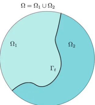
Fig. 4 A schematic illustration of domainwith two fluids separated by free interfacet

Consider domainwith two incompressible fluids occupying subdomains1 and 2 (see Fig.4) and t D 1 \2 free interface between the two fluids. Classical approach to this problem yields incompressible Navier-Stokes equation in each subdomain:

( i

ui_t Cui ruiC rpi Diui;

r ui _D0; ini: (33)

Define Cauchy stress tensori by the following relation [119]:

iui rpD r i with i DiruiCruiTpiI:

Then the position of the interface at each individual time is determined by the immiscibility condition

ui DVn (34)

and the Young-Laplace stress free (force balance) condition (see, for instance, [9]):

ΠD H ;

whereΠis the jump of the stress across the interfacet, with its normal,H the mean curvature of the surface, andthe surface tension constant. Also we assume no-slip condition both on the boundary and on the interface

ui D0on@; ŒuD0ont:

Z

t

VnΠdSxD Z

t

H Vn dSxD d

dtareat;

multiplying first equation in (33) by uiand integrating overiforiD1; 2, one can get the energy dissipation law:

d dt

" X

iD1;2 Z

i

1 2

ˇ

ˇuiˇˇdxCareat #

D X

iD1;2 Z

i

2i ˇ ˇ ˇ ˇ ˇ

rui CruiT 2

ˇ ˇ ˇ ˇ ˇ 2

dx:

(35)

4.2

Diffusive Interface Approximations (Phase Field Methods)

To regularize the transition between two phases, here the statistical point of view (or phase field approach) is employed, which treats the interface as a continuous, but steep, change of properties (density, viscosity, etc.) of the two fluids. Within a “thin” transition region, the fluid is mixed and has to store certain amount of “mixing energy.” Such an approach coincides with the usual phase field models in the theory of phase transition [24,25,95,98,117,128]. These models will allow the topological change of the interface [93] and have many advantages when simulating front motions [29]. Recently many researchers have employed the phase field approach for various fluid models [4,16,18,19,31,32,62,69,71,88,91,96,104].

Suppose that the interface t has thickness O."/. Then consider phase field satisfying

' .x/D (

1; in1

1; in2;

which takes values in.1; 1/on the diffusive interface.'may not necessarily be an obvious physical quantity (like concentration or volume fraction) but just a labeling function representing the smooth transition between phases.

Following [25], here the mixing energy is introduced as a functional of ' to approximate the interface term in the energy (35)

W.'/D

Z ₁

2jr'j 2

C 1

"2G .'/ dxareat; (36)

where G is a so-called double-well potential (e.g., G .'/ D 1₄'2₁2_{), " is} a parameter responsible for the “width” of the interface, and = depends on G .'/and"(for given example D 3"

phases). The competition between the two effects defines the profile of' across the interface.

Remark 16. The study of the physics of biological membranes of vesicles such as

cells and liposomes may involve more complicated forms of surface bending energy. One example of such elastic energy [46] may take the form:

ED

Z

k.H c0/2dS; (37)

where H D .k1C k2/=2is the mean curvature of the membrane surface, with k1 and k2 as the principle curvatures, k is the bending rigidity, and c0 is the spontaneous curvature that describes the asymmetry effect of the membrane or its environment. The equilibrium configuration of the vesicle membrane is determined by minimizing the above elastic bending energy with prescribed volume and surface area constraints. To approximate this energy by phase field, one can write

E".'/D 3 p

2k 16"

Z

"'C ₁

"'Cc0

p

2

1'2 2

dxI (38)

the volume of the region enclosed by the membrane will be determined by (V D

.jj C A.'//=2): A.'/ D R' dx; and the surface area of the membrane is determined by (up to a constant) B".'/ D

R

" 2jr'j

2 _C 1 4".'

2 _1/2_{dx: The}

original spontaneous curvature c0 is defined only on the surface (it may vary on the surface, representing a heterogeneity of the membrane). We extendc0 to the whole domainin a way that, in a neighborhood of,c0 is constant in the direction normal to. The equilibrium configuration is obtained by minimizing the above elastic bending energyE".'/with the constraints thatA.'/andB.'/are constants. See [46] for convergence ofE".'/toEas"!0.

More complicated form of elastic bending energy is a part of the Helfrich model, which has been studied extensively in the literature in recent years (see [34,102,113, 114] and additional references in [47]). This is also related to the classical Willmore problem in differential geometry [130].

Now, taking u to be incompressible background velocity (e.g., volume-averaged [1]), not the velocity of either of fluids, the following kinetic and Helmholtz free energy follows:

KD

Z _.'/j

uj2

2 dx; FDW.'/ : (39)

(introducing energy dissipation on the diffusive interface). If one takes microscopic dynamics to be that of gradient flow (and introducing appropriate dissipationD), variation produces Allen-Cahn/Navier-Stokes system, while to get the phase field to satisfy conservation law, one can introduce “Darcy’s like” dissipation (proportional to relative drag) and deduce Cahn-Hilliard/Navier-Stokes system.

4.2.1 Allen-Cahn/Navier-Stokes Systems

Here the following energy dissipation law is considered [67, modified viscous dissipation]:

d

dt .KCF/D Z

2 42 .'/

ˇ ˇ ˇ ˇ ˇ

ruC.ru/T 2

ˇ ˇ ˇ ˇ ˇ 2

C 1

j'tC.u r/ 'j 2

3 5dx;

(40) where K andF are taken from (39). There are two quantities of interest in this model: u and', so the variation will be performed for each of them separately.

First, we look at the microscopic dynamics on the interface given by Allen-Cahn equation [3]. It can be seen as gradient flow with convection in microscale variable':

'tC.u r/ ' D L2x;t_

ıR₀T .KCF/ dt ı'

!

To get this equation from energy dissipation law (40) as force balance for variable ', one may to notice that variation of kinetic energyR 1₂juj2dx gives inertial force

only when performed with respect to the flow map generated by u. So performing variation with respect to', the total energyKCFshould be treated altogether as Helmholtz free energy. So the variation goes as

ı'R₀TKCFdtDR₀TRh0.'/₂juj2ı'Cr' rı'C _"12G

0_{.'/ ı'}i_dxdt

DR₀TRh0.'/₂juj2 C'C _"12G0.'/

i ı'dxdt

CR₀TR_@.r' / ı' dSxdt:

Notation. Here we have two quantities of interest:'and u. So one has to adapt the variational notation to multiple variations of the same functional. Thus, here

ı' Z T

0

Kdt D lim

h!0 RT

0

K.'Chı';x/K.';x/

h dt;

ıx Z T

0

Kdt D lim

h!0 RT

0

K.';xChıx/K.';x/

h dt;

To cancel the boundary effects, one would make the boundary term in the variation equal to zero, which results in the boundary conditionr' D0. Then the force

balance (4) can be rewritten asL2 x;t_

ıR₀TKdt

ı' CL2x;t_ ıR₀TFdt

ı' CL2x_ıı'Dt D 0, which

reads as follows 8

< :

0.'/juj2

2 C

'C 1 "2G0.'/

C 1

.'tC.u r/ '/D0; x2;

r' D0; x2@:

Now, considering macro-scale background flow u yields the variation with respect to flow map x.X; t /. When writing macroscopic force balance, to account for “separation of scales,” one should consider microscopic variable ' to be transported with the flow, i.e., satisfy Eq. (9), so one has to include only viscous

part of dissipationD D R .'/ ˇ ˇ

ˇruC.2ru/T ˇ ˇ

ˇ2dx in the variation. Performing the

variation (subject to the assumption detF D1or equivalentlyr uD0) yields

ıxR₀TKdtDıxR₀TR1₂ .'0.X//jxt.X; t /j2dXdt

DR₀TRŒ .'/ .utC.u r/u/ıx dxdt;

ıxR₀TFdtDıxR₀TRh1₂ˇˇF1rX.'0/ ˇ ˇ2

C_"12G .'0/

i dXdt

DR₀TR Œr .r'˝ r'/ıxdxdt

R₀TR_@ .r' /r'ıxdSxdt;

ıuDDR

ruC.ru/T 2

WrıuC.rıu/Tdx

DRr hruC.ru/Tiıudx

CR_@rıuC.rıu/TW.ıu˝ / dSx:

Notation. For two matricesAandB, the scalar productAWBDP

i;j

Ai;jBi;j.

Remark 17. When taking the variation of kinetic energy K, one can perform

integration by parts (int) after changing the coordinates back to Eulerian. Then

the variation would result inL2 x;t_

ıR₀TKdt

ıx D . .'/u/t.u r/ . .'/u/.

Hence, force balance may be written asL2 x;t_

ıR₀TKdt

ıx DL

2 x;t_

ıR₀TFdt ıx CL

2 x_

ıD

ıu , which yields

.'/ .utC.u r/u/Crp D r h

and on the boundary, the condition uD 0is taken, which yieldsıuD 0, so takes care the boundary term.

Altogether this results in the Allen-Cahn/Navier-Stokes system [89]: 8 ˆ ˆ ˆ ˆ ˆ ˆ ˆ ˆ < ˆ ˆ ˆ ˆ ˆ ˆ ˆ ˆ :

'tC.u r/ ' D'_"12G

0_.'/ 2

0_.'/juj2

; x2;

.'/ .utC.u r/u/C rpD r h

ruC.ru/Ti

r .r'˝ r'/ ; x2;

r uD0; x2;

uD0; r' D0; x2@:

(42)

Remark 18. In order to get the system without the ₂0.'/juj2 term in the first equation, one can use 1₂Œ .'/ .utC.u r/u/C. .'/u/tC.u r/ . .'/u/as a convective term in the second equation.

4.2.2 Cahn-Hilliard/Navier-Stokes Systems

Now assume that phase field satisfies conservation law:

'tC r .'V/D0; (43)

and energy law [21]

d

dt.KCF/D Z

2 42 .'/

ˇ ˇ ˇ ˇ ˇ

ruC.ru/T 2 ˇ ˇ ˇ ˇ ˇ 2

C'2˝M1.'/ .Vu/; .Vu/˛ 3 5dx:

(44)

On macro-scale the variation is identical to the gradient flow case so gives Eq. (41). To perform variation on microscopic interfacial scale, one should define flow map x'.X; t /as@tx'DV and x'.X; 0/DX:We treat the macroscopic flow velocity u is fully independent from x'. And, as in gradient flow case, kinetic energy

Kis treated as a part of free energy. Using (10), one gets

ıx_'R₀T Kdt DıR₀TR1₂

'0.X/ det@_@xX'

juj2det@x_@X'dXdt

DR₀T R1₂rx'Œ

0_{.'/ ' .'/j}

uj2ıx'dxdt

DR₀T R'rh₂10_.'/juj2i_ı

x'dxdt;

ıx'

RT

0 Fdt Dı RT 0 R " 1 2 ˇ ˇ ˇ ˇF1rX

'0.X/ det@_@xX'

ˇˇ_ˇ ˇ 2

C _"12G

'0.X/ det@_@xX'

# dXdt

DR₀T R'r'C 1 "2G0.'/

ıx'dxdt

CR₀T R_@r ' ıx'

.r' /

C1 2jr'j

2_C''C 1

"2ŒG .'/'G0.'/ ıx'

ıVDDR'2M1.'/ .Vu/ ıVdx:

Thus, the force balance '2_M1_{.'/ .Vu/ C 'r'C}1 "2G

0_.'/

C1₂0.'/juj2iD0, combined with (43), leads to Cahn-Hilliard equation

'tC.u r/ ' D r ŒM .'/r ; D 'C 1 "2G

0_.'/C 1 2

0_.'/juj2 :

Force balance on the boundary gives r' D 0; V D 0 (second

condition yieldsıx' D0). Notice thatD L2x;t_ ıR₀TKdt

ı' CL2x;t_ ıR₀TFdt

ı' is the same variational gradient as in Allen-Cahn equation. All combined with boundary conditions leads to Cahn-Hilliard/Navier-Stokes system :

8 ˆ ˆ ˆ ˆ ˆ ˆ ˆ ˆ ˆ ˆ ˆ ˆ ˆ ˆ < ˆ ˆ ˆ ˆ ˆ ˆ ˆ ˆ ˆ ˆ ˆ ˆ ˆ ˆ :

'tC.u r/ ' D r ŒM .'/r ; x2;

D 'C_"12G0.'/C1₂0.'/juj

2 ;

.'/ .utC.u r/u/C rpD r h

ruC.ru/Ti

r .r'˝ r'/ ; x2;

r uD0; x2;

uD0; r' D0; M .'/r D0; x2@:

(45)

Remark 19. For the system (45), the phase field effective velocity V is defined up to a termV withQ r 'VQD0, which results in nonuniqueness of the energy law (44).

To eliminate this drawback, one may employ the operatorR D./1=2_{rand with} M D1consider the following energy dissipation law:

d

dt.KCF/D Z

2 42 .'/

ˇ ˇ ˇ ˇ ˇ

ruC.ru/T 2

ˇ ˇ ˇ ˇ ˇ 2

C jR.'V'u/j2 3 5dx:

Performing the variational procedure on this energy law, one would still get system (45).

Remark 20. To formally derive conservative Allen-Cahn/Navier-Stokes system,

d

dt .KCF/D Z

2 42 .'/

ˇ ˇ ˇ ˇ ˇ

ruC.ru/T 2 ˇ ˇ ˇ ˇ ˇ 2 C 1

jr .'V'u/j 2

3 5dx:

(46) Once again, macroscopic force balance yields Navier-Stokes equation (41), while microscopic force balance reads as

'r

1

r .'V'u/'C 1 "2G

0

.'/C 1

2 0

.'/juj2 D0;

or

r .'V/C.u r/ 'D

'C1

"2G 0

.'/C 1

2 0

.'/juj2 CC:

Integrating this equation overand using boundary conditions uD0;r' D

0;V D0yieldC D _j1_jR_"12G

0_.'/C1 2

0_.'/juj2

dx, which altogether give

nonlocal Allen-Cahn/Navier-Stokes system:

8 ˆ ˆ ˆ ˆ ˆ ˆ ˆ ˆ ˆ ˆ < ˆ ˆ ˆ ˆ ˆ ˆ ˆ ˆ ˆ ˆ :

'tC.u r/ ' D h

C 1 jj

R dx

i

; x2;

D 'C_"12G

0_.'/C1 2

0_.'/j uj2; .'/ .utC.u r/u/C rpD r

h

ruC.ru/Ti

r .r'˝ r'/ ; x2;

r uD0; x2;

uD0; r' D0; x2@:

(47)

4.3

Boundary Conditions in the Diffusive Interface Models

Authors of [105] have shown that the model with energy dissipation at the solid boundary surface better matches molecular dynamics experiments and avoids discrepancy of the contact line dynamics. More precisely, standard boundary conditions do not allow contact line to move along the boundary, while molecular dynamics experiments show that near-complete slip occurs in vicinity of contact line near the boundary.

Hence, one may consider the following expression for energy dissipation (includ-ing bulk terms already mentioned above):

DD 1₂R

2 .'/ˇ_ˇˇruC₂.ru/Tˇˇ_ˇ2C'2˝M1.'/ .Vu/; .Vu/˛dx

C1₂R_@ˇjuj2C 3" 2p2

j'tC.u r/ 'j 2