I. I NTRODUCTION C ONSIDER the initial value problems (IVP) x, y x0 , X yx0y(1) where fRm , can be solved using the hybrid linear multistep methods (HLMM)

High-order Hybrid Obreshkov Methods

R. I. Okuonghae

, and I. B. Aiguobasimwin

Abstract—In this paper, a family of high order Obreshkov hybrid formulas are proposed for the numerical solution of first order initial value problems (IVPs) in ordinary differ-ential equations (ODEs). These formulas are stable for step numberk≤18. Results from numerical experiments with the constructed hybrid methods on well-known stiff problems have been reported herein.

Index Terms—Continuous LMM, third derivative LMM, hybrid LMM, stiff problems, boundary locus, A(α)-stability.

I. INTRODUCTION

C

y′=f(x, y), x∈[x0, X], y(x0) =y0, (1)

wheref : R×Rm →Rm, can be solved using the hybrid linear multistep methods (HLMM)

yn+k=yn+k−1+h k

∑

j=0

βjf(xn+j, yn+j)

+

s

∑

r=1 hr

(_∑k

j=1

β_i,j(r)Dry(xn+vj, yn+vj)

)

, (2)

with the hybrid predictor,

yn+vi =

k

∑

j=0

αjyn+j+ s

∑

r=1 hr

(_∑k

j=1 β(i,jr)D

r

y(xn+j, yn+j)

)

,

wherekdenotes the step number,h=xn+1−xnis the step length, y′(xn+j, yn+j) =fn+j,Dry(xn+j, yn+j) =f

(r−1) n+j and Dr_y(x

n+vj, yn+vj) = f

(r−1)

n+vj . The vi in (2) is called

the off-step point and isv= [v1, v2,· · ·, vk]T. If the off-step points v1 ̸=v2 ̸=· · · ̸=vk, then the methods have Runge-Kutta’s flavour and is regarded as general linear methods (GLM [3]) withkstages, see [28]. Ifv1=v2=· · ·=vk=

v, then the formula in (2) is a GLM with single stage. The hybrid LMM in (2) is a constituent method of the so-called multiderivative LMM. As noted in [2], the multiderivative LMM was first proposed by Obreshkov in 1940, see [18]. The formulas in (2) offers the opportunity to bypass the Dahlquist order barrier for LMM [6]. The interest herein is to propose a method with an implicit structure. Methods of this kinds gives large stability region, high order and small error constant. These are advantages of hybrid methods over LMM. Several classes of hybrid LMM exist, see examples in [1], [2], [3], [4], [5], [7], [13], [14], [15], [17], [18], [19], [20], [21], [22], [23], [24], [25], [26], [27], [28], [29]. Stability issue is one of the main points to be considered

Manuscript received August 02, 2017; revised Nov 18, 2017.

∗_{Department of Mathematics,University of Benin, Benin City. Nigeria.} e-mail: (okunoghae01@yahoo.co.uk).

†Department of Mathematics,University of Benin, Benin City. Nigeria. e-mail:(becsin2002@yahoo.co.uk).

when constructing a constituent method in (2). Applying the method in (2) on the Dahlquist test problem:

y′=λy, y0= 1, Re(λ)<0, (3)

yields a stability polynomial

π(w, z) =wk−wk−1−z

k

∑

j=0 βjwj

− s

∑

r=1 zr

(_∑k

j=1 β_i,j(r)

(_∑k

j=0

αjwj+ s

∑

r=1 zr

k

∑

j=1 β(_i,jr)wj

))

. (4)

Herez=λh, and as in [16] and [31], the stability region of the method is defined to be

S={z∈C;|π(w, z)| ≤1}.

The use of appropriate Taylor expansions of {y(xn+j),

y′(xn+j),|j = 0(1)k, y′(xn+k), y′′(xn+k), y′′′(xn+k),

y′(xn+v),y′′(xn+v),y′′′(xn+v)} in (2a) and (2b) about the mesh pointxn reduces (2) to the form

L.T.Ek=Cpk+1h

pk+1_y(pk+1)_(x

n) +O(hpk+1),

L.T.Eq =C (q) pq+1h

pq+1_y(pq+1)_(x

n) +O(hpq+1),

q= 1,2,3,· · ·, k,whereL.T.E is the local truncation error of the methods, whilepq andpkare the order of the schemes in (2) alongside its hybrid predictor respectively. TheCpk+1

and C_p(q)

q+1 are the error constants of the methods in (2).

The LMM (2) is implicit, hence we solve the arising system of nonlinear algebraic equations in terms ofyn+k using the Newton Raphson iterative scheme

y_n(s₊+1)_k =y_n(s₊)_k−[F′(y(_ns₊)_k)]−1F(y(_ns₊)_k),

whereF′(y_n(s₊)_k) is the Jacobian matrix. The starter for the Newton Raphson scheme is the fourth order Runge-Kutta method (RKM).

In [10], a class of third derivative LMM was considered. The scheme in [10] is an extension of the Enright’s second derivative LMM[8]. The LMM were shown to beA(α)-stable for step numberk≤5 withαas the angle of stability. In a way, the LMM in [10] is a subclass of the method in (2). An example of the third derivative hybrid LMM (TDHLMM) in [27] is

yn+v = k

∑

j=0

αjyn+j+hβ (1)

k fn+k+h2β (2)

k fn′+k, (5)

with an output scheme,

yn+k=yn+k₋1+h k

∑

j=0

βjfn+j+hβv(1)fn+v

+h2βv(2)fn′+v+h 3

βv(3)fn′′+v. (6)

The hybrid LMM[27] in (6) is a constituent method of the hybrid multistep multi-derivative methods in (2). The order

IAENG International Journal of Applied Mathematics, 48:1, IJAM_48_1_11

of the predictor formula in (5) isp=k+ 2, while the order of the output scheme in (6) is p=k+ 4. The stability plot of the scheme in (5) and (6) shows that the formulas in (2) areA-stable fork≤3andA(α)-stable for step number4≤ k≤9. Their stability characteristics and the error constants are given in Table XI. The C_p(q)

q+1, and Cpk+1, pq, q = 1,

andpk(6)represent the error constants and the order of the methods in (5) and (6) respectively.

In this paper, a third derivative hybrid LMM

y(xn+vh) = k

∑

j=0

αj(v)yn+j+hβ (1) k (v)fn+k

+h2β(2)_k (v)f_n′_+k+h3β(3)_k (v)f_n′′_+k, (7)

y(xn+th) =yn+k−1+h k

∑

j=0

βj(t, v)fn+j

+hβ_v(1)(t, v)fn+v+h2βv(2)(t, v)fn′+v

+h3β_v(3)(t, v)f_n′′_+v, (8)

is proposed. The v = k− 1₂ in (7) and (8) represents the off-step point while the transformation variable t in (8) is t = (x−xn)/h. The approximations y(xn +vh) and {y(xn +th)}kt=1 are of order p = k+ 3 and p = k+ 4 respectively. The continuous coefficients{αj(v)}kj=0,

{β(_kr)(v)}3

r=1, {βj(t, v)}kj=0, and {β (r)

v (t, v)}3r=1 are poly-nomial of order less or equal top. To implement the formula in (8) compute the solution yn+v in (7) at the hybrid point

xn+v and substitute the resulting solution yn+v into the functionfn+v in the output method in (8) to obtainyn+k. In Section II we discuss the derivation of the hybrid predictor formula in (7) using collocation and interpolation techniques, see [21]. While Section III summarize the derivation of the output method in (8). In Section IV, an A(α)-stability analysis is provided. Four numerical experiments will be given in Section V to validate the aims of this paper.

II. DERIVATION OF THE HYBRID PREDICTOR FORMULA IN (7)

To derive the hybrid predictor formula, the solution of the IVPs is assumed to be the polynomial

y(x) =

N

∑

j=0

ajxj, (9)

where {xj}N_j=0 is the monomial polynomial basis function and {aj}Nj=0 are the real parameter constants to be deter-mined. SettingN =k+ 3, we have

    

y′(x) =∑N_j=1=k+3jajxj−1,

y′′(x) =∑N_j=2=k+3j(j−1)ajxj−2,

y′′′(x) =∑N_j=3=k+3j(j−1)(j−2)ajxj−3,

(10)

where y′(x) = f(x, y), y′′(x) = f′(x, y) and

y′′′(x) =f′′(x, y). Collocating (10) at{x=xn+j}kj=0, and interpolating (9) at x=xn+v, we obtain the linear system of equations

XA=B, (11)

where X=           

1 xn x2n x3n · · ·

1 xn+1 x2n+1 x3n+1 · · · ..

. ... ... ... · · ·

1 xn+k x2n+k x 3

n+k · · ·

0 1 2xn+k 3x2n+k · · ·

0 0 2 6xn+k · · ·

0 0 0 12 · · ·

· · · xk_n+3

· · · xk_n+3₊₁

..

. ...

· · · xk_n+3_+k

· · · (k+ 3)xk_n+2_+k

· · · (k+ 2)(k+ 3)xk_n+1_+k

· · · (k+ 1)(k+ 2)(k+ 3)xk n+k

           , A=            a0 a1 .. . ak

ak+1 ak+2 ak+3

          

, B=

           yn

yn+1 .. .

yn+k

fn+k

f_n′_+k f_n′′_+k

           .

Solving (11) the values of {aj}kj=0+3 are determined and substituting the resulting values a′_js into the polynomial representation (9) with further simplification yield the coefficients {αj(v)}kj=0, β

(1) 1 (v), β

(2) 1 (v), β

(3) 1 (v) in equation9, withv = (x−xn)/h andαv(v) = 1 on the left hand side of equation9 for a fixed value ofk. For example, settingk= 1 in (7) is the hybrid predictor formula

yn+v=α0(v)yn+α1(v)yn+1+hβ (1) 1 (v)fn+1

+h2β(2)₁ (v)f_n′₊₁+h3β(3)₁ (v)f_n′′₊₁. (12)

Again, for the method in (7), fixk= 1 in (11) to obtain

X=      

1 xn x2n x3n x4n

1 xn+1 x2n+1 x3n+1 x4n+1

0 1 2xn+1 3x2n+1 4x3n+1

0 0 2 6xn+1 12x2n+1

0 0 0 6 24xn+1

     , A=       a0 a1 a2 a3 a4     

, B=

      yn

yn+1 fn+1 f_n′₊₁ f_n′′₊₁

    

. (13)

Solving equation (13) for the values ofa0,a1,a2,a3,a4and substituting the resulting values a′_js and the transformation

t = v = (x−xn)/h into the polynomial representation (9) gives the method in (12) with continuous coefficients,

α0(v) =

(

1−4v+ 6v2_−4v3_+v4

)

,

α1(v) =

(

4v−6v2+ 4v3−v4

)

,

β(1)1 (v) =

(

−3v+ 6v2−4v3+v4

)

,

β(2)₁ (v) =

(

v−5v2 2 + 2v

3₋v4 2

)

,

β(3)₁ (v) =

( −v 6+ v2 2 − v3 2 + v4 6 ) .

IAENG International Journal of Applied Mathematics, 48:1, IJAM_48_1_11

Settingv= 1₂ in the continuous coefficients and substituting the resulting expressions into (12) gives

y_n+1 2 =

1 16

(

yn+ 15yn+1

) − 7

16hfn+1

+3 32h

2_f′ n+1−

1 96h

3_f′′

n+1, p= 4. (14)

Following these procedures we obtained the discrete coef-ficients of the method in (7) for step number k ≤ 18, see Tables IX, X, and XV.

III. THE HYBRIDLMMIN(8)

Using the ideas in section 2, we obtain a system of equation X=             

1 xn+k−1 x2n+k−1 x 3

n+k−1 · · ·

0 1 2xn 3x2n · · ·

0 1 2xn+1 3x2n+1 · · · ..

. ... ... ... · · ·

0 1 2xn+k 3x2n+k · · ·

0 1 2xn+v 3x2n+v · · ·

0 0 2 6xn+v · · ·

0 0 0 12 · · ·

· · · xk_n+4_+k−1

· · · (k+ 4)xk+3 n · · · (k+ 4)xk_n+3₊₁

..

. ...

· · · (k+ 4)xk_n+3_+k

· · · (k+ 4)xk_n+3_+v

· · · (k+ 3)(k+ 4)xk_n+2_+v

· · · (k+ 2)(k+ 3)(k+ 4)xk_n+1_+v

              , A=              a0 a1 a2 .. .

ak+1 ak+2 ak+3 ak+4

            

, B=

            

yn+k−1 fn

fn+1 .. .

fn+k

fn+v

f_n′_+v f_n′′_+v

             . (15)

Now, consider a case fork= 1in (8) yields

XA=B, (16)

where X=        

1 xn x2n x3n x4n x5n

0 1 2xn 3xn2 4x3n 5x4n

0 1 2xn+1 3x2n+1 4x3n+1 5x4n+1

0 1 2xn+v 3x2n+v 4x3n+v 5x4n+v

0 0 2 6xn+v 12x2n+v 20x3n+v

0 0 0 12 24xn+v 60x2n+v

        , A=         a0 a1 a2 a3 a4 a5        

, B=

        yn fn

fn+1 fn+v

f_n′_+v f_n′′_+v

        .

Solving (17) by MATHEMATICA software package we

obtain the values of {aj}5j=0. Substituting the resulting valuesa′_jsandt= (x−xn)/h into (9) yields

y(xn+th) =yn+hβ0(t, v)fn+hβ1(t, v)fn+1

+hβ_v(1)(t, v)fn+v+h2βv(2)(t, v)fn′+v

+h3β(3)v (t, v)fn′′+v, (17) where,

β0(t, v) =t

(

4t4_{+ 20v}3_{+ 20t}2_{v(1 +v)−10tv}2_{(3 +v)}

−5t3_{(1 + 3v)})_/20v3_, β1(t, v) =t2

(

−4t3_{+ 15t}2_v−20tv2_{+ 10v}3)_/Ψ 1,

Ψ1= 20(−1 +v)3, βv(3)(t, v) =t2

(

12t3_−30v2_{+ 20tv(2 +v)}

−15t2_{(1 + 2v)})_{/120(−1 +v)v,} βv(1)(t, v) =t2

(

4t3_{(1 + 3(−1 +v)v)−10v}2_{(3−8v+ 6v}2₎

+20tv(1−2v+ 2v3)_−5t2(_1−6v2_{+ 8v}3))_/Ψ 2,

Ψ2= 20(−1 +v)3v3, βv(2)(t, v) =−t2

(

10(2−3v)v2_+t3_{(−4 + 8v)}

+5t2_{(1 +v−5v}2_{) + 20tv(−1 +v+v}2₎)_/Ψ 3,

Ψ3= 20(−1 +v)2v2.

Inserting t = 1and v = 1₂ into the continuous coefficients of the formula in (17) gives

yn+1=yn+h

(

1 10fn+

4 5fn+1

2 +

1 10fn+1

)

+₆₀1h3_f′′ n+1

2 ,

p= 6.

(18)

Following this approach we obtain the discrete methods of the hybrid LMM in (8) of order k+ 5 for step number

k≤18, see Tables XVI, XVII, and XVIII for their discrete coefficients. The composition of (14) and (18) produces a family of stable methods.

IV. STABILITY OF THE METHODS

Substituting the hybrid solutions yn+v in (7) at hybrid points xn+v into the output method in (8) for a corresponding k, and applying the resultant method to the scalar test problem (4) yield the stability polynomial

π(w, z) =wk−wk−1−z∑k_j=0βjwj −zβv(1)

(_∑

k j=0αjw

j_+zβ(1)

k wk+z2β (2)

k wk+z3β (3) k wk

)

−z2_β(2) v

(_∑

k

j=0αjwj+zβ (1)

k wk+z2β (2)

k wk+z3β (3) k wk

)

−z3β(3)v

(_∑

k

j=0αjwj+zβ (1)

k w

k_+z2_β(2)

k w

k_+z3_β(3)

k w

k

)

.

where,w=eiθ, θ∈[0,2π]. Solving the stability polynomial equationπ(r, z) = 0for the values ofz, we obtain the roots of π(r, z) = 0 to be z1, z2 and z3. The boundary loci of the roots of the stability polynomial π(r, z) of the hybrid method in (8) reveals that the new algorithm in (8) are A-stable for k ≤ 3 and A(α)-stable for 4 ≤ k ≤ 18. For

k≥19, the hybrid LMM (8) is not stable. The exterior of the graphs in Fig. 1 are the stability regions of the composite methods in (8). The advantages of the hybrid LMM(8) over the hybrid LMM(6) are:

• The stable hybrid LMM (6) have step number k ≤ 9, while the step number of the hybrid LMM(8) is k ≤ 18. The hybrid LMM (8) thus have more stable methods than the hybrid LMM in (6).

• Also, the order of the hybrid predictor in (6) is one less than that of the hybrid LMM(8) for a givenk.

IAENG International Journal of Applied Mathematics, 48:1, IJAM_48_1_11

0

2

4

6

8

10

Re(z)

k = 1

k = 2

k = 3

k = 4

k = 7

k = 8

k =9

k =10

k =12 k =13 k =14

k = 5

k = 6

k =15

k =17

k =16 k =18

k =11

Fig. 1 The stability regions (exterior of the closed curves) of the hybrid method in (8);k≤18.

IAENG International Journal of Applied Mathematics, 48:1, IJAM_48_1_11

•The inclusion of the third derivative function (i.ey_n′′′_+k= f_n′′_+k) into the hybrid predictor formula in (6) to form formula (8) have accounted for these advantages, see Tables VIII, XII, XIII, XIV, and XV.

V. NUMERICAL EXAMPLES

Consider some numerical experiments to evaluate the accuracy of the hybrid LMM in (6) and (7). Methods considered for comparison are

• TDHLMM: The new proposed third derivative hybrid LMM of order p= 6 in (8).

• TDHLMM: The third derivative hybrid LMM of order

p= 6in [29] and is

      

yn+1 2 =

1 8

(

yn+ 7yn+1

) −3h

8fn+1+ h2

16fn′+1, p= 3, yn+1=yn+h

(

1 10fn+

4 5fn+1

2 +

1 10fn+1

)

+1 60h

3_f′′ n+1

2

, p= 6.

• TDBDF: The third derivative backward differentiation formula in [27],

yn+4= ₅₈₄₅1

(

−27yn+ 256yn+1−1296yn+2+ 6912yn+3

)

+996h 1169fn+4−

360h2

16 fn′+4+288h

3

5845fn′′+4, p= 6.

•TDMM: The third derivative multistep method of order

p= 6in [10], yn+3=y2+h

( ₁

810fn−4807 fn+1+13fn+2+129608813fn+3

)

−83h2

432fn′+3+17h

3

720fn′′+3, p= 6.

Tables III, IV, V and VI shows the results of our numerical experiments for the stiff IVPs:

Example 1 A stiff equation

  

y′=−104_{(y−sin(x)) +cos(x),} y(0) = 0, x∈[0,1],

y(x) =sin(x).

Example 2 A stiff system of equations

                  

y₁′ =−8y1+ 7y2, y₂′ = 42y1−43y2, y(0) =

(

1 8

)

,

x∈[0,15],

y1(x) = 2e−x−e−50x, y2(x) = 2e−x+ 6e−50x.

Example 3 A stiff system of equations

          

y₁′ =−0.1y2, y1(0) = 1, y₂′ =−10y2, y2(0) = 1, x∈[0,15],

y1(x) =e−0.1x, y2(x) =e−10x.

Example 4 A stiff system of equations

          

y1′ =y2, y1(0) = 1.01,

y₂′ =−100y1−101y2, y2(0) =−2, x∈[0,15]

y1(x) = 0.01e−100x+e−x, y2(x) =e−100x−e−10x.

We will integrate these problems using constant step size

h= 0.0001. The results from the hybrid LMM in (6), (8), TDMM [10] and the TDBDF in [29] are given in Tables I, II, III, IV, V, VI, VII, IX, X, XV, and XIX. Tables I, II shows the absolute error (Error = |y(xn)−yn|) while Tables III, IV, V, VI, VII, IX, X, XV, XIX depict the maximum error ({∥y(xn)−yn∥}n2=1). They(xn)andyndenote the exact and the approximate solutions respectively. The notationsF eval

and CPU time stand for function evaluations (including

TABLE I RESULTS FOREXAMPLE1

x Method Err(y(xn)−yn) 0.2 TDHLMM(8) 2.1375×10−4

TDHLMM(6) 1.9670×10−4 TDBDF[29] 2.2792×10−3 TDMM[10] 5.1312×10−3 0.4 TDHLMM(8) 2.0088×10−4 TDHLMM(6) 1.8487×10−4 TDBDF[29] 4.5544×10−3 TDMM[10] 9.9471×10−3 0.6 TDHLMM(8) 1.8001×10−4 TDHLMM(6) 1.6563×10−4 TDBDF[29] 6.6480×10−3 TDMM[10] 1.4366×10−2 0.8 TDHLMM(8) 1.5196×10−4 TDHLMM(6) 1.3981×10−4 TDBDF[29] 8.4767×10−3 TDMM[10] 1.8213×10−2 1.0 TDHLMM(8) 1.7860×10−4 TDHLMM(6) 1.0846×10−4 TDBDF[29] 9.9673×10−3 TDMM[10] 1.6691×10−2

derivatives), and time (measured in seconds) respectively. The results in Tables I, II shows that the new hybrid method in (8) perform better than the existing TDMM and TDBDF in [10] and [29] respectively in terms of accuracy and computational cost but compares favorably with the hybrid LMM in (6). This shows that there are potential usefulness of the new algorithm (8) when applied to oscillatory stiff problems for a fixed step size.

Again, the small error values recorded in Tables III, IV, V and VI, shows that the proposed hybrid LMM (8) compares with the hybrid LMM in (6) but outperform the TDBDF [29] and TDMM in [10] in terms of accuracy and computational cost. The numerical results given in Tables VII and XIX confirm the outperformance of the proposed TDHLMM in (8) over the existing TDBDF and the TDMM in terms of accuracy and computational cost but compares with the TDHLMM in (6).

VI. CONCLUSION

In this paper, a family of stable high order third derivative hybrid LMM for the numerical integration of stiff IVPs in ODEs (1) have been presented. The plot of the boundary locus of the roots of the stability polynomials in section IV shows that the high order hybrid formula (8) isA-stable for

k≤3andA(α)-stable for4≤k≤18. Atk≥19instability sets in. To attest the accuracy of the methods in (6) and (8) we compared their errors (see, Tables III-VI) and found that the hybrid LMM in (8) compares with the TDHLMM in (6) but is more accurate than the TDMM and TDBDF in [10] and [29] respectively on the stiff ODEs solved. Further more the hybrid LMM (8) are shown to contains more stable methods than the method in (6), TDBDF and TDMM, (see, [10], and [29]), and in a way these are advantages which hybrid LMM (8) have over the hybrid LMM (6), TDBDF [29] and TDMM [10].

IAENG International Journal of Applied Mathematics, 48:1, IJAM_48_1_11

TABLE II CONTINUATION OF TABLE I

x Method Feval CP U−time 0.2 TDHLMM(8) 7996 1.0755

TDHLMM(6) 7996 0.4893 TDBDF[29] 5997 0.3388 TDMM[10] 11994 0.4718 0.4 TDHLMM(8) 15996 2.2317 TDHLMM(6) 15996 0.6695 TDBDF[29] 11997 0.6750 TDMM[10] 23994 0.7227 0.6 TDHLMM(8) 23996 3.2989 TDHLMM(6) 23996 0.6336 TDBDF[29] 17997 0.9341 TDMM[10] 35994 1.0863 0.8 TDHLMM(8) 31996 3.0464 TDHLMM(6) 31996 1.2324 TDBDF[29] 23997 1.2198 TDMM[10] 47994 1.2566 1.0 TDHLMM(8) 39996 2.5181 TDHLMM(6) 39996 1.5431 TDBDF[29] 29997 1.6004 TDMM[10] 59994 1.6691

TABLE III RESULTS FOREXAMPLE2

x Method MaxErr(y(xn)−yn) 5 TDHLMM(8) 8.7794×10−15

TDHLMM(6) 8.1410×10−15 TDBDF[29] 1.3472×10−2 TDMM[10] 1.3476×10−2 10 TDHLMM(8) 1.1942×10−16

TDHLMM(6) 1.1159×10−16 TDBDF[29] 9.0808×10−5 TDMM[10] 9.0808×10−5 15 TDHLMM(8) 1.2093×10−18

TDHLMM(6) 1.1269×10−18 TDBDF[29] 6.1186×10−7 TDMM[10] 6.1186×10−7

TABLE IV CONTINUATION OFTABLE III

x Method Feval CP U−time 5 TDHLMM(8) 199996 20.5349

TDHLMM(6) 199996 20.2701 TDBDF[29] 149997 19.7722 TDMM[10] 299994 16.2736 10 TDHLMM(8) 399996 44.5201 TDHLMM(6) 399996 55.0782 TDBDF[29] 299997 72.8636 TDMM[10] 599994 57.9373 15 TDHLMM(8) 599996 135.0380

TDHLMM(6) 599996 140.5443 TDBDF[29] 499996 129.2100 TDMM[10] 899994 188.3261

TABLE V RESULTS FOREXAMPLE3

x Method MaxErr(y(xn)−yn) 5 TDHLMM(8) 5.1370×10−13

TDHLMM(6) 5.1370×10−13 TDBDF[29] 5.5118×10−1 TDMM[10] 4.6293×10−1 10 TDHLMM(8) 6.1251×10−13

TDHLMM(6) 6.1251×10−13 TDBDF[29] 4.7687×10−1 TDMM[10] 4.8877×10−1 15 TDHLMM(8) 5.5719×10−13

TDHLMM(6) 5.5719×10−13 TDBDF[29] 5.5354×10−1 TDMM[10] 4.8877×10−1

TABLE VI CONTINUATION OFTABLE V

x Method Feval CP U−time 5 TDHLMM(8) 199996 21.9943

TDHLMM(6) 199996 23.8431 TDBDF[29] 149997 18.8889 TDMM[10] 299994 21.3296 10 TDHLMM(8) 399996 71.0465 TDHLMM(6) 399996 77.4558 TDBDF[29] 299997 71.5335 TDMM[10] 599994 71.7773 15 TDHLMM(8) 599996 208.4335

TDHLMM(6) 599996 204.9257 TDBDF[29] 499996 193.5967 TDMM[10] 899994 185.6705

TABLE VII RESULTS FOREXAMPLE4

x Method MaxErr(y(xn)−yn) 5 TDHLMM(8) 1.4321×10−10

TDHLMM(6) 1.3479×10−10 TDBDF[29] 6.7386×10−3 TDMM[10] 6.7383×10−3 10 TDHLMM(8) 1.9299×10−12

TDHLMM(6) 1.8164×10−12 TDBDF[29] 4.5404×10−5 TDMM[10] 4.5404×10−5 15 TDHLMM(8) 1.9506×10−14

TDHLMM(6) 1.8358×10−14 TDBDF[29] 3.0593×10−7 TDMM[10] 3.0593×10−7

TABLE VIII CONTINUATION OF XII

k 18

p1 (7) 21

pk(8) 22

C_p(1) 1+1(7)

103385 2199023255552 Cp_k+1(8) _{6434279721678038630400000}−28075623577881641

α 530

IAENG International Journal of Applied Mathematics, 48:1, IJAM_48_1_11

TABLE IX

THE DISCRETE COEFFICIENTS OF THE HYBRID PREDICTOR IN(7),v=k−1₂

k 1 2 3 4 5 6 7 8

α0 1

16 − 1 512

1

3456 − 5 65536

7

256000 − 7 589824

33

5619712 − 429 134217728 α1 ₁₆15 ₃₂3 ₁₀₂₄−5 ₆₉₁₂7 ₁₃₁₀₇₂−45 ₅₁₂₀₀₀77 _1179648−91 _11239424495

α2 0 465

512 15 128 −

35 4096

7

3072 − 495 524288

1001

2048000 − 455 1572864 α3 0 0 24535_{27648 256}35 −₈₁₉₂105 ₁₈₄₃₂77 _1048576−2145 ₈₁₉₂₀₀1001 α4 0 0 0 1541015

1769472

315

2048 − 1155 65536

1001

147456 − 32175 8388608 α5 0 0 0 0 42125531_{49152000 4096}693 ₁₃₁₀₇₂−3003 ₉₈₃₀₄1001 α6 0 0 0 0 0 55382019_{65536000 16384}3003 −₅₂₄₂₈₈15015 α7 0 0 0 0 0 0 112546488769_{134873088000 32768}6435 α8 0 0 0 0 0 0 0 _{1150917017600}949434718947

β(1)k −167 −105

256

−1805 4608

−55685 147456

−300013 819200

−3505733 9830400

−335572523 963379200

−1401794537 4110417920 β(2)_k 3

32 21 256

115 1536

1715 24576

5397 81920

20559 327680

275847 4587520

1700127 29360128 β(3)k −961 −

1 128 −

5 768 −

35

6144 − 21

4096 − 77

16384 − 143

32768 − 2145 524288

TABLE X CONTINUATION OF TABLE IX

k 9 10 11 12 13

α0 _382205952715 _2097152000−2431 _55826186244199 _57982058496−29393 _14743817420852003 α1 _268435456−7293 13585

764411904 − 51051 4194304000

96577

11165237248 − 734825 115964116992 α2 _449576968415 _1073741824−138567 _101921587295095 _16777216000−1174173 _446609489922414425 α3 _9437184−7735 53295

89915392 − 969969 2147483648

2187185

6115295232 − 391391 1342177280 α4 _655360017017 _75497472−146965 _102760448159885 _17179869184−22309287 _4892236185654679625 α5 _16777216−109395 323323

65536000 − 205751 50331648

735471

205520896 − 111546435 34359738368 α6 _117964817017 _67108864−692835 _2621440002263261 _603979776−4732273 _8220835846128925 α7 _1048576−36465 _235929646189 _134217728−2078505 _5242880007436429 _1207959552−16900975 α8 109395_{524288 16777216}−692835 _12582912323323 _2147483648−47805615 _3355443207436429 α9 1369743780532699_{1678037011660800 1048576}230945 −_335544321616615 _2264924167436429 −_4294967296132793375 α10 0 5425625817417377_{6712148046643200 4194304}969969 _134217728−7436429 _90596966437182145 α11 0 0 27260350600663193_{34033786857455616} 2028117_8388608 −_26843545616900975 α12 0 0 0 16216534692600892117_{20420272114473369600} 16900975_67108864 α13 0 0 0 0 2827251526953679405285_{3589067026839839440896}

β(1)k −665887703040222757759081

−4376973241927 13317754060800

−49619129184677 153471261081600

−1172798911730641 3683310265958400

−15630801570008773 49798354795757568 β(2)_k 29582839

528482304

573713569 10569646080

584295049 11072962560

13661878997 265751101440

69339054385 1381905727488 β(3)k 3145728−12155 −

46189

12582912 − 29393

8388608 − 676039

201326592 − 1300075 402653184

TABLE XI

ANGLE OF STABILITY AND ERROR CONSTANTS OF THE HYBRID METHOD IN(5)AND(6).

k 1 2 3 4 5 6 7 8 9

p1 (5) 3 4 5 6 7 8 9 10 11

pk(6) 6 6 7 8 9 10 11 12 13

C_p(1) 1+1(5)

−1 384 −

1

1280 − 1

3072 − 1

6144 − 3

32768 − 11

196608 − 143

3932160 − 13

524288 − 221 12582912 Cp_k+1(6) ₈₀₆₄₀₀−1 ₈₀₆₄₀₀−1 _1411200−1 _58060800−23 _304819200−71 _114960384000−16601 _650496000−16 _{46030137753600}−2915333 _{74798973849600}−3307771

α 900 900 900 780 760 750 730 690 670

TABLE XII

ANGLE OF STABILITY AND ERROR CONSTANTS OF THE METHOD IN(8).

k 1 2 3 4 5 6 7 8

p1 (7) 4 5 6 7 8 9 10 11

pk(8) 6 6 7 8 9 10 11 12

C(1)_p 1+1(7)

1 3840

1 15360

1 43008

1 98304

1 196608

11 3932160

13 7864320

13 12582912 Cp_k+1(8) ₈₀₆₄₀₀−1 ₈₀₆₄₀₀−1 _1411200−1 _58060800−23 _304819200−71 _114960384000−16601 _650496000−16 _{46030137753600}−2915333

α 900 ₉₀0 ₉₀0 ₈₉0 ₈₈0 ₈₈0 ₈₄0 ₈₄0

Fork= 18in (7), the coefficients are:

α0=−_{267181325549568}21607465 , α1=_{337618789203968}618759225 , α2=−_{562949953421312}11197545975 ,

IAENG International Journal of Applied Mathematics, 48:1, IJAM_48_1_11

TABLE XIII CONTINUATION OF XII

k 9 10 11 12 13

p1 (7) 12 13 14 15 16

pk(8) 13 14 15 16 17

C_p(1) 1+1(7)

17 25165824

323 704643072

323 1006632960

7429 32212254720

2185 12884901888 Cp_k+1(8) _{74798973849600}−3307771 _{466279317504000}−14810423 _{5711921639424000}−133516991 _{7170658550415360000}−125975989493 _{483734902210560000}−6505755121

α 830 780 770 760 730

TABLE XIV CONTINUATION OF XII

k 14 15 16 17

p1(7) 17 18 19 20

pk(8) 18 19 20 21

C_p(1) 1+1(7)

2185 17179869184

3335 34359738368

20677 274877906944

227447 3848290697216 Cp_k+1(8) _{83380417624229806080000}−872467295136263 _{14144892275538984960000}−116819976368363 _{5125443318665891020800000}−33841462074966061 _{249153494657369702400000}−1330405884897877

α 690 ₆₄0 ₆₂0 ₅₇0

TABLE XV CONTINUATION OF TABLE IX

k 14 15 16 17

α0 _736586891264−185725 _402653184007429 _{70368744177664}−9694845 _{168809394601984}17678835 α1 _2948763484161404081 _{1473173782528}−5386025 _80530636800230299 _{140737488355328}−319929885 α2 _17179869184−734825 _{1179505393664}40718349 _{5892695130112}−166966775 _{11785390260224}1836634525 α3 _8932189798421729825 _103079215104−21309925 _{2359010787328}420756273 _{11785390260224}−1836634525 α4 _10737418240−10567557 _714575183872630164925 _824633720832−660607675 _{18872086298624}13884957009 α5 _362387865610935925 _107374182400−306459153 _{1429150367744}3907022535 _549755813888−1453336885 α6 _137438953472−1003917915 317141825

43486543872 −

3166744581 429496729600

3907022535 519691042816 α7 _11509170176165480975 _274877906944−4159088505 _869730877441404485225 −_85899345920014928938739 α8 _2147483648−50702925 4798948275

184146722816 −

128931743655 4398046511104

15449337475 463856467968 α9 _67108864022309287 _12884901888−490128275 _36829344563216529710725 −_{8796093022208}472749726735 α10 _17179869184−717084225 646969323

13421772800 −

3038795305 51539607552

109096090785 1473173782528 α11 _671088643380195 −_343597383681890494775 _268435456001823277183 −_343597383683038795305 α12 −_2147483648152108775 98025655

1610612736 −

19535112675 274877906944

20056049013 214748364800 α13 _13421772835102025 −_4294967296339319575 _3221225472233753485 −_54975581388849589132175 α14 2909581849195234436929

3721995435241314975744

145422675

536870912 −

1502700975 17179869184

367326905 4294967296 α15 0 17330788171545842816113_{22331972611447889854464 1073741824}300540195 −_343597383683305942145 α16 0 0 4405974680902572131447189

5716984988530659802742784

9917826435 34359738368 α17 0 0 0 1303230166670878624419129605_{1702275590827341309750018048}

β(1)_k −_{7377534043815936}2284668726871879 −_{44265204262895616}13534484747796343 −_{5665946145650638848}1711609253590902955 −_{99239905217759674368}29636518134678098123

β(2)k 4299262263296210885500055

412887721357 8598524526592

25899879459329 550305569701888

78549071042067 1700944488169472 β(3)k −

1671525

536870912 − 3231615

1073741824 − 100180065

34359738368 − 194467185 68719476736

α3= _12884901888017733023 , α4=−_{13469017440256}9183172625 , α5=_{37744172597248}97194699063 ,

α6=−_{6597069766656}50866790975 , α7=_{1039382085632}19535112675 , α8=−_{2748779069440}104502571173,

α9= _{8349416423424}540726811625, α10=−_{35184372088832}3309248087145, α11=_42090679500849589132175,

α12=−_824633720832106357835675, α13= 10799411007_85899345920, α14=−_{2199023255552}247945660875,

α15= _257698037762571288335, α16=−_{1099511627776}115707975075, α17=20419054425_68719476736,

α18=2219937586898787493495038475_{2918186727132585102428602368}, β (1)

18 =−150754631232181010575510376655405621182464, β (2)

18 = 97196827895398444084062779215,

β(3)18 =−274877906944756261275 .

The following are the coefficients of the output method in (8) fork= 16,k= 17, andk= 18. (i). Fork= 16,

β0= _{9059822965698785280000}116819976368363 , β1=−_{51919041192742563840000}13956304648392919 , β2=_{1256588962320384000}3363331121369 ,

β3=−_{38014093877760000000}644150257220081 , β4= _{740027968337129472000}56698655109648907 , β5=−_{104310673600573440000}27489914255435927 ,

IAENG International Journal of Applied Mathematics, 48:1, IJAM_48_1_11

TABLE XVI

THE DISCRETE COEFFICIENTS OF THE HYBRIDLMMIN(8),v=k−1₂,αk₋1

k 1 2 3 4 5 6 7 8

β0 1

10 0 − 1 105000

1

288120 − 23 15746400

71

100623600 − 1277 3372969600

61 277200000 β1 ₁₀1 ₁₀1 ₇₅₆₀1 ₂₁₀₀₀−1 _10372320197 _110224800−1013 _26564630400134951 _8769720960−27037

β2 0 1

10 27 280

1

2520 − 251 1890000

89

1481760 − 53593 1616630400

109999 5312926080 β3 0 0 ₈₄₀83 ₁₂₀11 ₄₀₈₂₄₀323 ₃₇₈₀₀₀−107 _19559232028349 _64665216−5833

β4 0 0 0 41

420

373 4320

67

51030 − 257447 498960000

1657 5588352 β5 0 0 0 0 ₁₅₁₂₀₀14599 ₁₅₁₂₀₀12203 _59875200117349 _2494800000−2117323 β6 0 0 0 0 0 ₅₀₄₀₀4819 _199584001494589 _1197504032693 β7 0 0 0 0 0 0 _199584001891723 _3991680275201

β8 0 0 0 0 0 0 0 ₁₉₉₅₈₄18769

β9 0 0 0 0 0 0 0 0

β10 0 0 0 0 0 0 0 0

β(1)v 45 4 5

95048 118125

2188888 2701125

24114649792 29536801875

923974447552 1123242379875

2884271941216384 3480179306979375

26980916685133952 32315950707665625 βv(2) 0 0 ₇₈₇₅−8 ₂₅₇₂₅−64 _93767625−392992 _324168075−1951232 _77260057875−611554688 _717414823125−7064897536 βv(3) ₆₀1 ₆₀1 ₁₇₅3 ₇₃₅13 ₂₉₇₆₇₅5426 ₉₃₅₅₅1754 _171517533008 _15926625314032

TABLE XVII CONTINUATION OF TABLE XVI

k 9 10 11 12

β0 _{21415347233280}−2915333 _{37372243708800}3307771 _{247150455552000}−14810423 _{3182094807091200}133516991 β1 16375189

8172964800000 − 29377501 21415347233280

8776683037

8969338490112000 −

8736730187 12110372322048000 β2 _399022303680−5603183 _3891888000003930029 _{98840064153600}−749651389 _{8969338490112000}52837290067

β3 5173

82223856 − 6278089 133007434560

1564845703

42032390400000 − 620939779 20395568793600 β4 _25219434240−5190203 _3139456320498221 _{95765352883200}−12503042077 _{73556683200000}8246055859 β5 19301089

35597802240 − 1941229 4670265600

1323575927

3767347584000 −

2317483453 7366565606400 β6 _579150000751819 _3559780224032532173 _{22697490816000}−17417190937 _342486144000241704167 β7 5920261

1634592960 − 8896331 4729725000

3092332951

2135868134400 −

210041550619 158882435712000 β8 _29059430418285433 _10897286405049431 _{10897286400000}−28479964621 _{29902153881600}65322964829 β9 406999627

4358914560

35402761 622702080

40703130877

7061441587200 −

114813631883 32691859200000 β10 0 _217945728002021767051 _1868106240009480425729 _{1008777369600}7073607469 β11 0 0 _1005903360009275408641 _{1307674368000}58351960643

β12 0 0 0 _21794572800019985454563

β(1)v 255162484027663392912896_{303406155994940683059375} 5934957111166001015951872_{7006945535250162104728125} 1452322809448761532933213184_{1702687765065789391448934375 1014099400439777739023176865625}870946527423481017196690045952 β(2)v 396213141100651875−4673778456310784 −

6621134890442752

481592403829411875 −

1836932372218502144

117026954130547085625 −

53443468107108573184 3030425252765145860625 β(3)v _51740826637510435184224 _993005763752045479264 _{8043346686375}169001355136 _{9055795919625}193859604352

β6= _{2085909359260446720000}1496775485341589891 , β7=−_{17577717009076224000}27949043222289253 , β8=_{236532139683840000}692811308413337 ,

β9=−_{71953076891824128000}328813048682276341 , β10= _{36797642873671680000}226573220046911879 , β11=−_{8211044277596160000}60360531225279253 ,

β12= _{20862134720114688000}169386146453044553 , β13=−_{304112751022080000}2762410962625387 , β14=_{60822550204416000}800235952475431 ,

β15= _{2128789257154560000}42669914521521979 , β16= _{266098657144320000}23947293120218047, β (3)

v = _{5104507653402782625}116653376406728704,

β(1)v =_{103946449589267750763518564715334700377265625}91647257011056661100920335813512624923639808, β (2)

v =−_{23034657528872960525456579803125}581527530758995096960223936512 . (ii). Fork= 17,

β0=−_{3366101179511990599680000}33841462074966061 , β1= _{930141824478408622080000}203761802665292947 , β2=−_{190369817706722734080000}434709687227056061 ,

β3= _{376253508925963468800}5703429870536141 , β4=−_{15556362822000000000}1119711571443371 , β5=_{6783589709757020160000}1766231524933031561 ,

β6=−_{30980270059370311680000}23122430770999469281 , β7= _{4867121838274375680000}8478451544842042733 , β8=−_{863466800445849600}2916581095040731 ,

β9=287386549715865600000015896620515789544031 , β10=−17131684974243840000133079759712391799 , β11=2120245137006796800002017775517276730301 ,

β12=−_{1219340075223029760000}12703020446237718811 , β13= _{478090587335961600}5080317638037319 , β14=−_{10270474486272000000}113478084449170457 ,

β15= _{48634646874992640000}728389418194688563 , β16= _{31222242438266880000}434057127890848013 , β17=_{4460320348323840000}399790748392466023,

βv(1)= 7532424483990211083325457297861835258586430308352_{8489826270203443543610378773124961653313169921875}, βv(2)=−_{1881355653670699050916666155420234375}50995220028659329462315246200291328 ,

βv(3)= _{416910662591672270896875}9666279146678627885056 .

IAENG International Journal of Applied Mathematics, 48:1, IJAM_48_1_11

TABLE XVIII CONTINUATION OF TABLE XVI

k 13 14 15

β0 _{4168212048000000000}−125975989493 −_{21608011256832000}46580217381683 _{51919041192742563840000}−872467295136263 β1 1773875194229

3245736703233024000 −

20769720941 49037788800000000

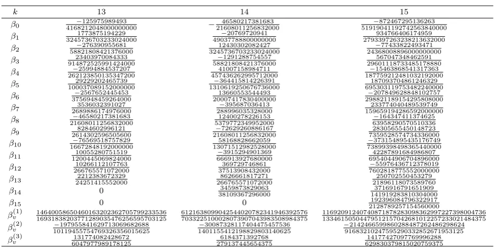
934766406174959 2793397263238213632000 β2 _{58821808421376000}−276390955681 _{3245736703233024000}12430302082427 _{24368008896000000000}−77433822493471 β3 _{914872525991424000}23403970084333 _{58821808421376000}−1291288754557 _{29601118733485178880}567047348462591 β4 _{262123850135347200}−25994884537207 _{457436262995712000}41007158984711 _{187759212481032192000}−15463868541317363 β5 _{100037089152000000}29229202465739 _{1310619250676736000}−364415814226391 _{695303119753482240000}187093704861246329 β6 _{3756948459264000}−2567652445453 _{20007417830400000}13660553544493 _{298821189154295808000}−207849628848102757 β7 _{2689886174976000}3536032391027 _{288996035328000}−395687036413 _{159659194286592000000}233774040489539749 β8 _{21608011256832000}−46580217381683 _{5379772349952000}12400278226153 _{63958290570510336}−164347411374625 β9 _{2614302596505600}8284602996121 _{21608011256832000}−72629260886167 _{7359528574734336000}28305655450148723 β10 _{16672848192000000}−76569518757829 _{13071512982528000}58168828662059 _{73899398498365440000}−373154895435176749 β11 _{1200445069824000}10055280751519 _{666913927680000}−3915294901369 _{6954044906704896000}42287891684986807 β12 _{266765571072000}10266112107763 _{37513908432000}369729746861 _{7602818775552000000}−55976436712378019 β13 _{24251415552000}2212383672329 _{266765571072000}8626661817271 _{21896118073589760}250702550453279 β14 0 _{38109367296000}3459873829063 _{141919283810304000}3716916791651909 β15 0 0 _{2128789257154560000}192396084796322917 β(1)v 1464005865046016320236270579923353616931838203771289035476256595703125

6121638099042544020782341946392576 7033225100028073907043983508984375

11692091240740871878283098362997227398004736 13346150504479512157042681012257233021484375 β(2)v _{10119455754769326356015625}−197955841629713069682688 _{1401155412198829803140625}−30087328117404475457536 −_{91683210247595290332852671953125}2142466599860288487262486298624 β(3)v _{6047977989178125}131774082428672 _{279137445654375}6184371392768 _{629830379815020759375}14177427097769996288

TABLE XIX CONTINUATION OF TABLE VII

x Method Feval CP U−time 5 TDHLMM(8) 199996 16.7258

TDHLMM(6) 199996 22.0396 TDBDF[29] 149997 86.7256 TDMM[10] 299994 105.9252 10 TDHLMM(8) 399996 86.0563

TDHLMM(6) 399996 77.3734 TDBDF[29] 299997 182.7800 TDMM[10] 599994 136.5398

15 TDHLMM(8) 599996 198.86123 TDHLMM(6) 599996 210.7978

TDBDF[29] 449997 221.5977 TDMM[10] 899994 191.1616

(iii). Fork= 18,

β0=_{167331705567586560000000}1330405884897877 , β1=−_{134644047180479623987200}24343072174033957 , β2=_{14309874222744748032000}28187363165850683 ,

β3=−_{7614792708268909363200}104237283655215653 , β4= _{92182109686861049856000}6282590727626358889 , β5=−_{83765030580000000000}21687070030031627 ,

β6=_{1356717941951404032000}1058893586336440273 , β7=−_{43372378083118436352000}83178007336587302171 , β8=_{51232861455519744000}200664850158837391 ,

β9=−_{536139516616704000}3619605412337437 , β10= _{14369327485793280000000}142991357900432776627 , β11=−_{263827948603355136000}3352161742062834863 ,

β12= _{296834319180951552000}4236180286887090343 , β13=−_{243868015044605952000}3517654171116544631 , β14=_{66932682227034624000}914796569714599841 ,

β15=−_{975695076195840000000}12951640426824528679, β16=_{126450081874980864000}2138075007773440481 , β17=_{1248889697530675200}9699147218622149 ,

β18= _{6244448487653376000}557578398333615829, β (1)

v = 821260448868871592798480340859013392989565878272_{919950215037524842186883148790630519708857421875},

βv(2)=−_{203862067735215067436790450277734375}5901262231296627471263170306244608 , βv(3)= _{45176077989809688796875}1062006198320978354176.

IAENG International Journal of Applied Mathematics, 48:1, IJAM_48_1_11

ACKNOWLEDGMENT

The authors would like to thank the anonymous referees for their helpful comments and valuable suggestions, which led to the improvement of the manuscript.

REFERENCES

[1] J. C. Butcher, “A modified multistep method for the numerical integra-tion of ODEs”,J. Assoc. Comput. Mach. 12, (1965), 124-135. [2] J. C. Butcher,The Numerical Methods for Ordinary Differential

Equa-tions, John Wiley and Sons Ltd, Chichester, 2008.

[3] J. C. Butcher, “Some new hybrid methods for IVPs”. In. J. R. Cash and Glad Well (eds), Computational ODEs, Clarendon press, Oxford, 29-46, 1992.

[4] J. C. Butcher, and A. E. O’Sullivan, “Nordsieck methods with an off-step point”.Numerical Algorithms, 31, 87-101, 2002.

[5] W. B. Gragg, and H. J. Stetter, “Generalized multistep predictor corrector methods”,J. Assoc. Comput. Mach., 11, pp.188-209, 1964. [6] G. Dahlquist, “On stability and error analysis for stiff nonlinear

problems”,Part 1, Report No TRITA-NA-7508, Dept. of Information processing, Computer Science, Royal Inst. of Technology, Stockholm, 1975.

[7] J. O. Ehigie and S. A. Okunuga, “L(α)-stable second derivative block formula for stiff initial value problems,” IAENG International Journal of Applied Mathematics, vol. 44, no.3, pp. 157-162, 2007.

[8] W. H. Enright, “Second derivative multistep methods for stiff ODEs”.,

SIAM. J. Numer. Anal., pp. 321-331, 1974.

[9] W. H. Enright, T. E. Hull, and B. Linberg, “Comparing numerical methods for stiff of ODEs systems”.,BIT, 15, pp. 10-48, 1975. [10] A. K. Ezzeddine, and G. Hojjati, “Third Derivative Multistep Methods

for Stiff systems,”Intern. J. of Nonlinear Science., Vol.14, No.4, pp.443-450, 2012.

[11] S. O. Fatunla,Numerical Methods for Initial Value Problems in ODEs., Academic Press, New York, 1978.

[12] W. C. Gear, The automatic integration of stiff ODEs. pp. 187-193 in A.J.H. Morrell (ed). Information processing 68:Proc. IFIP Congress. Nort-Holland, Amsterdam, Edinurgh 1968.

[13] W. C. Gear,Numerical initial value problems in ordinary differential equations. Prentice-Hall Inc., Englewood Cliffs, 1971.

[14] E. Hairer, and G. Wanner, “Multistep-multistage-multiderivative meth-ods for ordinary differential equations,”Computing, Vol.11, pp. 287-303, 1973.

[15] E. Hairer, and G. Wanner,Solving Ordinary Differential Equations II. Stiff and Differentila-Algebraic Problems., Springer-Verlag, Berlin, 1996.

[16] H. Liu, and J. Zou, “Some new additive Runge-Kutta methods and their applications”.J. Comp. Applic. Maths., 190, (2006), 74-98. [17] J. J. Kohfeld, and G.T. Thompson, “Multistep methods with modified

predictors and correctors.”,J. Assoc. Comput. March., 14, pp.155-166, 1967.

[18] J. D. Lambert,Numerical Methods for Ordinary Differential Systems. The Initial Value Problems., Wiley, Chichester, 1991.

[19] J. D. Lambert, Computational Methods for Ordinary Differential Systems. The Initial Value Problems. Wiley, Chichester, 1973. [20] R. I. Okuonghae,Stiffly Stable Second Derivative Continuous LMM

for IVPs in ODEs. Ph.D Thesis. Dept. of Maths. University of Benin, Benin City. Nigeria. 2008.

[21] R. I. Okuonghae, S. O. Ogunleye, and M.N.O. Ikhile, “Some explicit general linear methods for IVPs in ODEs,”J. of Algor. Comp. Tech., Vol. 7, No.1, 41-63, 2013.

[22] R. I. Okuonghae, “Variable order explicit second derivative general linear methods,”Comp. Applied Maths, SBMAC, 33, 243-255, 2014. [23] R. I. Okuonghae, and M. N. O. Ikhile, “On the construction of high

orderA(α)-stable hybrid linear multistep methods for stiff IVPs and ODEs,”Journal of Numerical Analysis and Applications. No.3, Vol. 15, pp. 231-241, 2012.

[24] R. I. Okuonghae, and M. N. O. Ikhile, “Second derivative general linear methods,”Numerical Algorithms, Vol. 67, issue 3, pp. 637-654, 2014.

[25] R. I. Okuonghae, and M. N. O. Ikhile, “A class of hybrid linear multistep methods with A(α)-stability properties for stiff IVPs in ODEs,”J. Numer. Math.,Vol. 21, No.2, pp. 157-172, 2013.

[26] R. I. Okuonghae, and M. N. O. Ikhile, “A-stable high order hybrid linear multistep methods for stiff problems,”J. of Algor. Comp. Tech.

Vol.8, No.4, pp.441-469, 2014.

[27] R. I. Okuonghae, M.N.O. Ikhile, and J. Osemeke, “An off-step-point methods in multistep integration of stiff ODEs,” NMC Journal of Mathematical Sciences., Vol. 3, No.1, pp. 731-741, 2014.

[28] R. I. Okuonghae, and M. N. O. Ikhile, “Third derivative GLM for stiff problems.”J. Nig. Assoc. Maths. Physics., Vol.26, pp.58-65, 2014. [29] R. I. Okuonghae, and V. Akhimien, “A Note on High Order A(α

)-stable Third Derivative Backward Differentiation Formulas for Stiff Systems.,”J. Nig. Assoc. Maths. Physics., Vol.28, No. 2, pp. 101-106, 2014.

[30] U. W. Sirisena, P. Onumanyi, and J. P. Chollon, “Continuous hybrid through multistep collocation,” ABACUS, Vol. 28; No. 2; pp. 5866, 2002.

[31] O. Widlund, “A note on unconditionally stable linear multistep meth-ods.”,BIT,7: 65-70, 1967.

IAENG International Journal of Applied Mathematics, 48:1, IJAM_48_1_11