Quasi-Newton Methods for the Acceleration of Multi-Physics Codes

Quasi-Newton Methods for the Acceleration of

Multi-Physics Codes

Rob Haelterman, Alfred Bogaers, Joris Degroote, Nicolas Boutet

Abstract—Often in nature different physical systems interact which translates to coupled mathematical models. Even if pow-erful solvers often already exist for problems in a single physical domain (e.g. structural or fluid problems), the development of similar tools for multi-physics problems is still ongoing. When the interaction (or coupling) between the two systems is strong, many methods still fail or are computationally very expensive. Approaches for solving these multi-physics problems can be broadly put in two categories: monolithic or partitioned. While we are not claiming that the partitioned approach is panacea for all coupled problems, here we will only focus our attention on studying methods to solve (strongly) coupled problems with a partitioned approach in which each of the physical problems is solved with a specialized code that we consider to be a black box solver and of which the Jacobian is unknown. We also assume that calling these black boxes is the most expensive part of any algorithm, so that performance is judged by the number of times these are called.

Running these black boxes one after another, until convergence is reached, is a standard solution technique and can be considered as a non-linear Gauss-Seidel iteration. It is easy to implement but comes at the cost of slow or even conditional convergence. A recent interpretation of this approach as a root-finding problem has opened the door to acceleration techniques based on quasi-Newton methods. These quasi-Newton methods can easily be “strapped onto” the original iteration loop without the need to modify the underlying code and with little extra computational cost.

In this paper, we analyze the performance of ten acceleration techniques that can be applied to accelerate the convergence of a non-linear Gauss-Seidel iteration, on different multi-physics problems.

Index Terms—Partitioned methods, iterative methods, quasi-Newton.

I. INTRODUCTION

O

Mathematically these can be written as the non-linear system

Manuscript received August 03, 2017.

R. Haelterman is associate professor at the Royal Military Academy, Dept. Mathematics, Renaissancelaan 30, B-1000 Brussels, Belgium. email: [email protected]

A. Bogaers is senior researcher at the Council for Scientific and Indus-trial Research, Advanced Mathematical Modelling, Modelling and Digital Sciences, Meiring Naud´e Road; Brummeria, Pretoria, South Africa and a visiting lecturer at the School of Computer Science and Applied Math-ematics, University of Witwatersrand, Johannesburg, South Africa. email: [email protected]

J. Degroote is associate professor at Ghent University, Dept. Flow, Heat and Combustion Mechanics, Sint-Pietersnieuwstraat 41, 9000 Ghent, Belgium. email: [email protected]

N. Boutet is PhD student at Ghent University, Dept. Flow, Heat and Combustion Mechanics, Sint-Pietersnieuwstraat 41, 9000 Ghent, Belgium and Royal Military Academy, Dept. Mathematics, Renaissancelaan 30, B-1000 Brussels, Belgium. email: [email protected]

of equations given by

        

f1(x1, x2, . . . , xn) = 0

f2(x1, x2, . . . , xn) = 0

.. . fn(x1, x2, . . . , xn) = 0

(1)

where fi : DF ⊂ Rm → Rki _{and x}

j ∈ Rmj _{(i, j ∈} {1,2, . . . , n}),Pn_i=1ki =m,Pn_j=1mj =m.

Each equation describes (the discretized equations of) a physical problem that is spatially or mathematically decomposed. E.g. f1(x1, x2) = 0 could give the pressure x1 on the wall of a flexible tube for a given geometry x2, whilef2(x1, x2) = 0, could give the deformed geometry of that same wall under influence of the pressure exerted on it by the fluid.

In this paper, we will assume the problem has the follow-ing characteristics [14], [20]:

1) Good solvers exist for each equation of the system. For this reason, we will use a partitioned solution method, i.e. each (system of) equation(s) will be solved separately.

2) The analytic form offi (i= 1,2, . . . , n) is unknown,

preventing the use of Newton’s method, for instance. 3) The problem has a large dimensionality, often imposing

the use of matrix-free implementations.

4) Evaluating fi (i = 1,2, . . . , n) is computationally

costly, preventing line-search techniques and matrix free Newton-Krylov techniques. This also means that the required number of evaluations (or “calls”) to reach convergence is a good proxy of the performance of an algorithm.

II. FIXED-POINT FORMULATION AND QUASI-NEWTON ACCELARATION

A typical solution method for (1) is the fixed-point itera-tion [21].

IAENG International Journal of Applied Mathematics, 47:3, IJAM_47_3_17

Fixed-point iteration

1. Startup:

1.1. Take initial valuesx1

2,x13, . . .x1n.

1.2. Sets= 1.

2. Loop until convergence:

2.1. Solvef1(x1, xs2, . . . , xsn) = 0 forx1,

resulting in xs₁+1.

2.2. Solvef2(xs₁+1, x2, . . . , xsn) = 0for x2,

resulting in xs₂+1. . . .

2.n. Solvefn(xs1+1, x

s+1

2 , . . . , xn) = 0 forxn

resulting in xsn+1.

2.n+1. Sets=s+ 1.

If F0 (the Jacobian of F = (f1, . . . , fn)) satisfies the

condition

∀i < j < n: [F0]ij = 0 (2)

then we can write the whole process 2.1. to 2.n, as xs+1

n =

H(xs

n)[19]. The problem can now be considered as finding

the fixed point of H, or alternatively as finding the zero of K(xn) =H(xn)−xn. It is at this root-finding problem that

we can apply quasi-Newton (QN) acceleration as follows.

Quasi-Newton acceleration

1. Startup:

1.1. Take initial valuesx12,x13, . . .x1n.

1.2. Sets= 1.

2. Loop until convergence:

2.1. Solvef1(x1, xs2, . . . , xsn) = 0 forx1, resulting in xs₁+1.

2.2. Solvef2(xs1+1, x2, . . . , xsn) = 0for x2, resulting in xs₂+1.

. . .

2.n. Solvefn(xs1+1, x

s+1

2 , . . . , xn) = 0 forxn

resulting in H(xs n).

2.n+1. Compute an approximate JacobianKˆ_s0 of K (see below)

2.n+2.xs+1

n =xsn−( ˆKs0)−1K(xsn)

2.n+3. Sets=s+ 1.

Alternatively a slightly different quasi-Newton step xs+1

n = xsn −Mˆs0K(xsn) can be used. Here Ms0 serves as

an approximation to the inverse of the Jacobian at step s, whereas Kˆ_s0 is an approximation of the Jacobian itself. We will designate methods that approximate the Jacobian as Type I methods, and methods that approximate the inverse Jacobian as Type II methods [14].

III. DIFFERENT CHOICES OF QUASI-NEWTON METHODS

We define δxs=xsn+1−xsn, δKs=K(xsn+1)−K(xsn)

and{ıj;j= 1, . . . , mn}as the canonical (orthonormal) basis

for Rmn_.

A. Non-Linear Gauss-Seidel (GS)

This method (also called, among others, “Iterative Sub-structuring Method” or “Picard iteration”) is nothing else than the fixed-point iteration described at the beginning of §II. It is seldom considered to be a quasi-Newton method, but can take this form if we set( ˆK0

s)−1=−I [21].

B. Aitken’sδ2 _{method (Aδ}2₎

Aitken’sδ2_{method [1] is a relaxation method and as such} again seldom seen as a quasi-Newton method, it can take its form if we define( ˆK_s0₊₁)−1₌₋ 1

ωs+1I with

ωs+1=

−ωs

hK(xs−n 1), K(xsn)−K(xs−n 1)i

hK(xs

n)−K(x s−1

n ), K(xsn)−K(x s−1

n )i

, (3)

whereh·,·iis the standard Euclidean scalar product.

C. Broyden’s first method (BG)

Broyden’s first (or “good”) method is a quasi-Newton method that is part of the family of Least Change Secant Update (LCSU) methods [5], [6], [10], [11], [15], where the approximate JacobianKˆ_s0₊₁ is chosen as the solution of the following minimization problem:

min{kKˆ0−Kˆ_s0kF r}, s.t. Kˆ0δxs=δKs. (4)

In other words, it gives a new approximate Jacobian that is closest to the previous one in the Frobenius norm and that satisfies the secant equation.

The solution of (4) leads to the following rank-one update:

ˆ

K_s0₊₁ = Kˆ_s0 +(δKs− ˆ

Ks0δxs)δxTs

hδxs, δxsi

(5)

ˆ

K₁0 is typically set to be equal to −I, which means that the first iteration equals a GS iteration.

Interpreting Broyden’s good method differently, we could say that

• Kˆ_s0₊₁ is the projection w.r.t. the Frobenius norm ofKˆ_s0

onto{A∈Rmn×mn_:Aδx

s=δKs};

• no change occurs betweenKˆ_s0₊₁andKˆ_s0 on the orthog-onal complement of δxs, i.e. ( ˆKs0+1 −Kˆs0)z = 0 if

hz, δxsi= 0.

We have the following properties of this method: 1) For linear problems, the method is known to show

superlinear convergence [21] and it needs at most2mn

iterations to reach the solution (Gay’s theorem [16]). 2) No guarantee can be given that the approximate

Jaco-bians are non-singular nor that convergence is mono-tone.

Using the Sherman-Morrison theorem [28], Broyden’s good method can be written as:

( ˆK_s0₊₁)−1=

( ˆK_s0)−1+(δxs−( ˆK

0

s)−1δKs)δxTs( ˆKs0)−1

hδxs,( ˆKs0)−1δKsi

(6)

ifhδxs,( ˆKs0)−1δKsi 6= 0.

IAENG International Journal of Applied Mathematics, 47:3, IJAM_47_3_17

D. Broyden’s second method (BB)

Broyden’s second (or “bad”) method is a quasi-Newton method that uses an approximationMˆ0 of the inverse Jaco-bian.

It is also part of the family of LCSU methods [5], [11], [15], where the approximate inverse Jacobian Mˆ_s0₊₁ is cho-sen as the solution of the following minimization problem:

min{kMˆ0−Mˆ_s0kF r}, s.t.Mˆ0δKs=δxs. (7)

i.e. it gives a new approximation of the inverse of the Jacobian that is closest to the previous one in the Frobenius norm and that satisfies the secant equation.

The solution of (7) leads to the following rank- one update

ˆ

M_s0₊₁= ˆM_s0+(δxs− ˆ

M_s0δKs)δKsT

hδKs, δKsi

. (8)

Interpreting Broyden’s bad method differently, we could say that

• Mˆ_s0₊₁ is the projection w.r.t. the Frobenius norm ofMˆ_s0

onto{A∈_Rmn×mn_:AδK

s=δxs};

• no change occurs between Mˆ_s0₊₁ and Mˆ_s0 on the

or-thogonal complement ofδKs, i.e. ( ˆMs0+1−Mˆs0)z= 0

if hz, δKsi= 0.

Broyden himself [5] admitted that this formulation of his algorithm didn’t function properly. The reasons for the “good” or “bad” behavior are not well understood, and it is quite possible that in some instances the bad method outperforms the good method. Indeed, as we will see, this is exactly what happens in some of the test-cases that we have examined.

We also have the following properties of this method:

1) For linear problems, the method is known to show superlinear convergence [21] and it needs at most2mn

iterations to reach the solution (Gay’s theorem [16]). 2) No guarantee can be given that the approximate inverse

Jacobians are non-singular nor that convergence is monotone.

Again, Mˆ₁0 is typically set to be equal to −I, which means that the first iteration equals a non-Linear Gauss-Seidel iteration.

E. Switched Broyden method (SB)

As Broyden’s Good method is not always better than Broyden’s Bad method, we follow an idea suggested in [23] that avoids the need to choose between the two methods and create a switched version of BG/BB (called “SB”) in the following manner. If

|δxTsδxs−1| |δxT

s( ˆKs0)−1δKs|

< |δK

T sδKs−1| δKT

sδKs

(9)

then (6) is used for the update, otherwise (8) is used. The idea behind this criterion is that it selects the update that would result in the smallest error with respect to previous secant equations.

F. Column-Updating Method (CU)

The Column-Updating method is a quasi-Newton method that was introduced by Martinez [24], [26], [27]. The rank-one update of this method is such that the column of the approximate Jacobian corresponding to the largest coordinate of the latest increment δxs is replaced in order

to satisfy the secant equationKˆ0δxs=δKsat each iteration.

The resulting method to update the approximate Jacobian is defined as follows:

ˆ

Ks0+1= ˆKs0 +

(δKs−Kˆs0δxs)ıTjK,s hıjK,s, δxsi

, (10)

whereıjK,s is chosen such that

jK,s= Argmax{|hıj, δxsi|;j= 1, . . . , mn}. (11)

This can be viewed as a rank-one update, where only the jK,s-th column of the approximate Jacobian is altered.

The methods starts from an educated guess Kˆ₁0, which is often set to−I.

The properties of this method have been investigated in [18], [24], [26]. It has to be noted that this method does not belong to the family of the LCSU methods, but it satisfies the hypotheses of Gay’s theorem [16] such that finite convergence is reached in at most2mn iterations for linear

problems.

This method can also be directly applied to( ˆK_s0)−1_{, using} the Sherman-Morrison theorem ifhıjK,s,( ˆK

0

s)−1δKsi 6= 0.

( ˆK_s0₊₁)−1=

( ˆK_s0)−1+(δxs−( ˆK

0

s)−1δKs)ıTjK,s( ˆK

0 s)−1

hıjK,s,( ˆK

0

s)−1δKsi

(12)

G. Inverse Column-Updating Method (ICU)

The Inverse Column-Updating method (ICU) is a quasi-Newton method that was introduced by Martinez and Zam-baldi [22], [25]. It uses a rank-one update such that the column of the approximation of the inverse of the Jacobian corresponding to the largest coordinate of δKs is replaced

in order to satisfy the secant equationMˆ0δKs=δxsat each

iteration.

The resulting method to update the approximate Jacobian is defined as follows:

ˆ

M_s0₊₁= ˆM_s0+(δxs− ˆ

M_s0δKs)ıTjM,s hıjM,s, δKsi

, (13)

whereıjM,s is chosen such that

jM,s= Argmax{|hıj, δKsi|;j= 1, . . . , mn}. (14)

This can be viewed as a rank-one update, where only the jM,s-th column of the approximate inverse Jacobian is

altered.

The methods starts from an educated guess Mˆ10, which is

IAENG International Journal of Applied Mathematics, 47:3, IJAM_47_3_17

often set to −I.

The properties of this method have been investigated in [22]. The method does not belong to the family of the LCSU methods, but it satisfies the hypotheses of Gay’s theorem [16] such that finite convergence is reached in at most2mn

iterations for linear problems.

H. Switched (Inverse) Column-Updating Method (SCU)

As far as the authors are aware, the idea behind SB has not been applied to CU and ICU, even though it is straightforward. As with SB, we use the condition (9) at every iteration. When it is satisfied, then CU (equation (12)) is used, otherwise ICU (equation (13)).

I. Non-linear Eirola-Nevanlinna Type I method (EN1)

It is clear from the different update formulas for the approximate Jacobian of BG, BB, SB, CU, ICU and SCU that they can only be applied starting with Kˆ₂0. In other words,Kˆ₁0 needs to be chosen. Conventionally, this is set to be equal to −I. Likewise, for Aδ2_{, ω1 needs to be chosen} and is set to 1. As a result all of the methods given above will have an identical first iteration, i.e.x2_n=H(x1_n).

The nonlinear Eirola-Nevanlinna was proposed by [32] as the nonlinear counterpart to the linear EN algorithm [13] and is different as it computes Kˆ10 based on a virtual choice of

ˆ

K00, set to be equal to −I (which can also be interpreted as setting the initial approximation of the Jacobian ofH as zero), which is used to create a first approximationKˆ0

1. The method is given by

( ˆK_s0₊₁)−1= ( ˆK_s0)−1+(ps−( ˆK0s)

−1_q s)pTs( ˆK

0

s)

−1

hps,( ˆKs0−1)−1qsi , (15) ps= −( ˆKs0)−1K(xsn+1), (16)

qs= K(xsn+1+ps)−K(xsn+1). (17)

Note that the EN algorithm requires two calls of K (or H) per iteration.

J. Non-linear Eirola-Nevanlinna Type II method (EN2)

Eirola and Nevanlinna did not propose a Type II method, but by generalisation this can be written as [14]:

ˆ

M_s0₊₁= Mˆ_s0+(ps−( ˆK0s)

−1_q s)qsT

hqs,qsi , (18)

whereps andqsare defined as in the EN1 method.

K. Switched Eirola-Nevanlinna method (SEN).

As far as the authors are aware, the idea behind SB has not been applied to EN1 and EN2, even though it is straightforward. As with SB, we use the condition (9) at every iteration. When it is satisfied, then EN1 (equation (15)) is used, otherwise EN2 (equation (18)).

IV. FLUID STRUCTURE INTERACTION TEST-CASES

Quasi-Newton methods have received significant attention in recent years within the field of partitioned fluid-structure interactions (FSI). QN methods have been shown to be an efficient and robust coupling procedure, especially in the context of black-box fluid and solid solvers. In this section we aim to investigate the various QN methods when applied to a number of incompressible, transient, FSI benchmark problems. The selected problems are all generally considered to be strongly coupled, difficult to solve FSI problems, requiring the use of implicit coupling strategies.

The problems are solved here by coupling OpenFOAM [31], an open-source, finite-volume based fluid flow solver, and Calculix [12], an open-source finite-element based solver for the structural domain deformations. Interface information, in the form of fluid stresses and solid displacements are transferred between the two domains using radial basis function interpolation using a consistent formulation [4], [7]. One of the primary aims of this investigation is to com-pare the performance of the various QN methods when the Jacobian, at the start of each new time step,k+ 1, is either reset to−I, such that

ˆ K₁0

−1

k+1=−I, (19) (which we will call “Jacobian re-set”) or set equal to the final approximation from the previous time step

ˆ K₁0

−1

k+1=

ˆ K_s0

−1

k , (20)

wherek indicates the time step counter (which we will call “Jacobian re-use”). A similar procedure is used for quasi-Newton methods usingMˆ₁0 and for Aitken’s method. A relaxation factor ofω= 0.001is used for the first iteration of the first time step, or for the first iteration in every time step whenever the Jacobian is reset such that

x1n =x

0

n+ωδxs. (21)

This is done to avoid the possibility of an excessively large first displacement guess, which can lead to divergence for strongly coupled problems. Furthermore, at the start of each new time step, x0

n is approximated by extrapolating the

interface state from the three preceding time steps, as was previously suggested in [9], using a polynomial of the form

x0_n,k+1= 5 2x

s n,k−2x

s n,k−1+

1 2x

s

n,k−2. (22)

A. Dynamic piston-channel problem

The piston-channel test problem layout is shown in Fig-ure 1, and consists of a 10m long fluid domain which is forced out of the domain by an accelerating unit by unit moving block. The problem is a surprisingly difficult problem to solve when using partitioned solutions schemes, and has been investigated in a number of publications (see for example [2], [8]). The coupling strength is sufficiently strong that simple fixed-point iterations, such as Gauss-Seidel iterations, are insufficient to guarantee convergence.

While the test case is intrinsically a one dimensional problem, it is modelled here in three dimensions, with a fluid domain discretised using 10 linear elements and a single

IAENG International Journal of Applied Mathematics, 47:3, IJAM_47_3_17

Fig. 1: Piston-channel test problem layout.

(a) (b)

Fig. 2: The interface (a) displacement and (b) velocity for the piston-channel test problem for a time step size of∆t= 0.02s, compared to the simplified 1D mass-spring system.

linear structural element. The fluid density and viscosity is 1kg/m3 and 1.0kg/(m s) respectively where the solid is described by a linear elastic material with a Young’s modulus ofE = 10.0Pa with a zero density and Poisson’s ratio. A slip boundary condition is applied to the fluid wall boundaries and the block velocity is prescribed asu(t) = 0.2t.

The simulation is solved here using time step sizes of ∆t= 0.02s for a convergence tolerance of = ||K_√(xsn)||

n =

10−8_{. The interface displacement and velocity, along with a} 1D-solution is shown in Figure 2. The 1D-model is found by simplifying the problem to a 1D mass-spring system, where the solid piston represents a linear spring and the fluid domain a variable mass (see [2] for more information on the simplified 1D-model). The accuracy of the FSI simulation can naturally be improved by increasing the mesh resolution or decreasing the time step size.

The average number of iterations required to reach con-vergence for each of the QN methods is summarised in Table I. The results highlight the surprising complexity of the test problem, with both GS and Aitken failing to provide convergent results. The performance of all the other QN methods is virtually identical, with a minor improvement offered by retaining the Jacobian at the start of each new time step.

B. Dam Break with an elastic obstacle

The dam break problem consists of a collapsing column of water striking an elastic baffle, which has previously analysed in [3], [30]. The problem setup is shown in Figure 3, and consists of a 29.2cm column of water which collapses under gravity, striking an 8cm tall, 1.2cm wide, elastic obstacle.

The problem is solved using a time step size of ∆t = 0.001s, where the fluid domain is discretised using 3670 linear fluid elements, and the solid domain discretised using 14 quadratic, full integration finite-elements. The advancing

TABLE I: The mean number of iterations required to reach convergence for the piston-channel test problem. Failure to converge is indicated by div() where the time step at which failure occurred is indicated in brackets, and the top performing method for each setting is highlighted in bold.

Jacobian re-use Jacobian re-set

GS N/A div(1)

Aδ2 _{div(1) div(1)}

BG 3.98 4.39

BB 3.98 4.38

SB 3.97 4.39

CU 3.98 4.39

ICU 3.98 4.39

SCU 3.98 4.39

EN1 3.91 6.92, div(276) EN2 3.90 6.99, div(285) SEN 3.89 6.91, div(276)

Fig. 3: Dam break with elastic obstacle problem description.

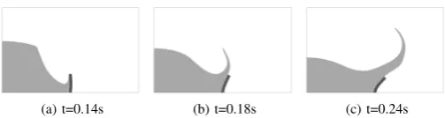
front along with the corresponding elastic deformation is shown in Figure 4 with a plot of the beam tip displacement shown in Figure 5.

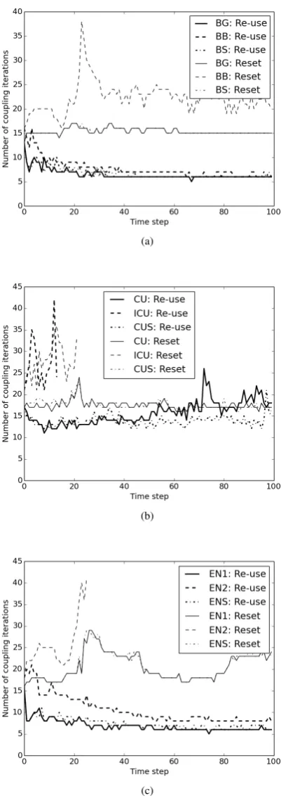
The mean number of iterations required by the various QN methods to reach convergence is shown in Table II. The Broyden family of methods is the top performing family of methods, with significant benefit seen in retaining the Jacobian from the previous time step. The convergence rate of all the QN methods, at time step 200 is shown in Figure 6(a) and highlights the comparative inefficiency of GS and Aitken’s method. Overall, switched-Broyden is the top performing QN method for this particular problem, and for illustrative purposes we show the number of iterations required in each time step in Figure 6(c), both when re-using or resetting the Jacobian.

C. Wave propagation in a three dimensional elastic tube

The 3D flexible tube problem was originally proposed in [17], inspired by the type of flow encountered in

haemo-(a) t=0.14s (b) t=0.18s (c) t=0.24s

Fig. 4: Wave interaction with elastic obstruction after dam break at various time steps.

IAENG International Journal of Applied Mathematics, 47:3, IJAM_47_3_17

Fig. 5: Beam tip displacement results for the dam break test problem, compared to the results reproduced from [30].

TABLE II: Mean number of iterations required by the QN methods for the dam break test problem. Failure to converge is indicated by div() where the time step at which failure occurred is indicated in brackets, and the top performing method for each setting is highlighted in bold.

Jacobian re-use Jacobian re-set

GS N/A 23.42

Aδ2 _{5.34, div(279) 6.33}

BG 4.17 5.99

BB 4.32 5.97

SB 4.14 6.05

CU 5.62 6.50

ICU 5.84 6.34

SCU 4.80 6.55

EN1 4.37 6.93

EN2 4.58 6.96

SEN 4.58 6.94

dynamics. The density ratios of the fluid and solid are near unity, which in conjunction with internal incompressible flow results in a very strongly coupled FSI problem, and as a result has received much attention in literature [2], [8], [9], [17].

The problem consists of a flexible tube of lengthl= 5cm, with an inner and outer radius ofri= 0.5cmandr0= 0.6cm respectively. The flexible tube is modelled using a St. Venant-Kirchoff material model, with a Young’s modulus of E = 3×106 _dynes/cm2_{, density ρ = 1.2 g/cm}3 _{and Poisson’s} ratio of 0.3, where the fluid flow has a density of ρ= 1.0 g/cm3 _{and a viscosity of µ = 0.03 poise. The problem is} modelled using 600 twenty noded quadratic solid elements coupled with 6000 linear fluid flow elements resulting in an interface Jacobian size of mn = 1880. The tube walls are

fixed on both ends, and a smoothly varying pressure in the form of

p(t) =

  

1.3332×104

(sin(2πt

0.003+32π)+1)

2

ift <0.003

0 ift≥0.003,

(23) is applied at the inlet. The time step size for the simulation is ∆t= 0.0001s with a convergence tolerance= ||K_√(xsn)||

n =

10−8. The resulting pressure pulse propogation is illustra-tively shown for different time steps in Figure 7.

The mean number of iterations over the first 100 time

(a)

(b)

(c)

Fig. 6: (a) Illustrative convergence rates for each of the QN methods when re-using the Jacobian at the start of each time step for the dam break test problem, shown here for time step 200. (b) The same convergence plot with GS and Aitken’s method removed to allow for better differentiation. (c) A comparison of the number of iterations required in each time step using switched Broyden, for both the re-use and reset case.

IAENG International Journal of Applied Mathematics, 47:3, IJAM_47_3_17

Fig. 7: Pressure pulse propagation at 0.003s, 0.005s and 0.008s (where the wall displacement is magnified by a factor 10).

TABLE III: Comparison of the mean number of iterations required to reach convergence for the 3D flexible tube test problem. Failure to converge is indicated by div() where the time step at which failure occurred is indicated in brackets, and the top performing method for each setting is highlighted in bold.

Jacobian re-use Jacobian re-set

GS N/A div(1)

Aδ2 _{div(1) div(1)}

BG 6.51 15.36

BB 7.68 22.25

SB 6.75 15.38

CU 15.63 17.51

ICU 27.21, div(14) 27.64, div(22)

SCU 13.89 17.62

EN1 6.91 20.56

EN2 10.56 16.83, div(26)

SEN 7.37 20.63

steps is shown in Table III for the various QN methods. The Broyden family of methods is once again the top performing method, with a clear benefit in retaining the old Jacobian at the start of each time step. A summary of the number of coupling iterations required per time step, for each of the family of methods, is shown in Figure 8. Out of all the test cases analysed in this paper, this problem most clearly highlights the inherent training that occurs by retaining and continuously adding onto the Jacobian. To further illustrate this inherent training, we show the convergence rates for Broyden’s good method in Figure 9 at different time steps for both re-use and resetting of the Jacobian.

D. 2D flexible beam fluid-structure interactions

The selected test problem consists of flow around a fixed cylinder with an attached flexible beam. The beam undergoes large deformations induced by oscillating vortices formed by flow around the circular bluff body. The problem was first proposed by Turek et al. [29], and has received substantial numerical verification.

The problem layout and material properties are provided in Figure 10(a) and consists of a 0.02m thick, 0.35m long flexible beam, attached to a fixed cylinder with diameter of 0.1m. The cylinder center is by design positioned to be non-symmetric with respect to the channel to remove

(a)

(b)

(c)

Fig. 8: A comparison of the number of coupling iterations required to reach convergence for the 3D flexible tube test problem when using (a) Broyden’s family of methods, (b) Column updating family of methods and (c) Eirola-Nevanlinna family of methods when re-using the Jacobian from the previous time step and when resetting the Jacobian to−I.

IAENG International Journal of Applied Mathematics, 47:3, IJAM_47_3_17

(a)

(b)

Fig. 9: Illustrative convergence rates at various time steps for the 3D flexible tube test problem using Broyden’s Good method when (a) re-using the Jacobian at the start of each time step and (b) when re-setting the Jacobian to −I at the start of the new time step.

dependence on numerical errors to induce the onset of deformations. A parabolic inlet boundary condition, with mean flow velocity of U¯ = 1m/s is slowly ramped up for t < 0.5s via (1−cos (πt/2))/2. The top, bottom and fixed cylinder walls are defined as non-slip boundaries. The problem is solved here using 3800 finite-volume fluid cells, and 72 full integration, quadratic finite elements.

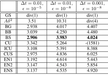
We investigate three different settings, namely for a com-paratively large time step size of∆t= 0.01s for two different convergence criteria of = 10−5 _{and = 10}−8 _{in order} to gain some insight into the convergence behaviour of the various QN methods as well as for a small time step size of ∆t= 0.001s for = 10−8_{. The beam tip displacement for} both time step sizes over the full simulation window is shown in Figure 10(b) with a snapshot of the beam displacement at 8.7s shown in Figure 10(c). The convergence behaviour for the various QN methods is summarised in Tables IV-Table V. Overall, switched Broyden outperforms all the QN methods across all three settings, with the switched strategies providing improved performance for both the conventional EN and CU methods.

(a)

(b)

(c)

Fig. 10: (a) Flexible beam problem description, (b) beam tip displacement over the 10s simulation window, and (c) beam displacement and pressure contours at 8.7 seconds.

TABLE IV: The mean number of iterations to reach con-vergence for the flexible tail benchmark problem for the various QN methods when the Jacobian is re-used. Failure to converge is indicated by div() where the time step at which failure occurred is indicated in brackets, and the top performing method for each setting is highlighted in bold.

∆t= 0.01, ∆t= 0.01, ∆t= 0.001, = 10−5 = 10−8 = 10−8

GS div(1) div(1) div(1)

Aδ2 _{3.51 10.31 div(4)}

BG 2.938 4.017 4.407

BB 3.039 4.250 4.480

BS 2.906 3.983 4.024

CU 3.342 5.264 -(1581)

ICU 3.108 5.391 8.388

CUS 2.975 4.836 6.025

EN1 3.192 4.614 5.443

EN2 3.147 4.543 5.854

ENS 3.137 4.535 4.920

V. CONCLUSION

We have tested a wide variety of acceleration techniques on four different multi-physics problems that are written as a fixed-point problem. While the choice of the best method remains problem dependent, it is clear that the best choice is the class of quasi-Newton methods, of which, more often than not, the tried and trusted Broyden method comes out on top.

Re-using the Jacobian of all the QN methods at the beginning of the iterations of the next time step results in important reductions in the required number of iterations. With a few exceptions, a switching strategy, that hasn’t drawn much attention in the past, is shown to offer a slight boost of perfor-mance in exchange for a negligeable penalty in complexity. The class of Eirola-Nevanlinna methods, which are among

IAENG International Journal of Applied Mathematics, 47:3, IJAM_47_3_17

TABLE V: The mean number of iterations to reach conver-gence for the flexible tail benchmark problem for the various QN methods when the Jacobian is re-set. Failure to converge is indicated by div() where the time step at which failure occurred is indicated in brackets, and the top performing method for each setting is highlighted in bold.

∆t= 0.01, ∆t= 0.01, ∆t= 0.001, = 10−5 _{= 10}−8 _{= 10}−8

GS div(1) div(1) div(1)

Aδ2 _{4.504 11.459 -(5)}

BG 4.170 6.617 6.872

BB 3.879 6.518 7.369

BS 4.196 6.611 6.920

CU 4.499 7.165 8.295

ICU 4.323 7.042 9.158

CUS 4.500 7.168 8.275

EN1 4.879 7.605 8.793

EN2 7.632 7.583 8.448

ENS 4.879 7.605 8.795

the lesser known QN methods, have not shown their worth, and in the authors’ opinion do not seem to warrant the complexity that they entail.

REFERENCES

[1] A.C. Aitken, On Bernouilli’s numerical solution of algebraic equations. Proc. Roy. Soc. Edinb.46, pp. 289–305 (1926)

[2] A.E.J. Bogaers, S. Kok, B.D. Reddy, T. Franz, Quasi-Newton methods for implicit black-box FSI coupling Computer Methods in Applied Mechanics and Engineering,279, pp. 113–132 (2014)

[3] A.E.J. Bogaers, S. Kok, B.D. Reddy, T. Franz, An evaluation of quasi-Newton methods for application to FSI problems involving free surface flow and solid body contactComputers & Structures,173, pp. 71–83 (2016)

[4] A.E.J. Bogaers, S. Kok, B.D. Reddy, T. Franz, Interface information transfer between non-matching, nonconforming interfaces using radial basis function interpolationTenth South African Conference on Com-puttional and Applied Mechanics, Potchefstroom, South Africa(2016) [5] C.G. Broyden, A class of methods for solving nonlinear simultaneous

equations.Math. Comp.19, pp. 577–593 (1965)

[6] C.G. Broyden, Quasi-Newton methods and their applications to function minimization.Math. Comp.21, pp. 368–381 (1967)

[7] A. de Boer, A.H. van Zuijlen, H. Bijl, Comparison of conservative and consistent approaches for the coupling of non-matching meshes

Computer Methods in Applied Mechanics and Engineering,197/49, pp. 4284–4297 (2008)

[8] J. Degroote, K.-J. Bathe, J. Vierendeels, Performance of a new par-titioned procedure versus a monolithic procedure in fluid–structure interactionComputers & Structures,87/11, pp. 793–801 (2009) [9] J. Degroote, R. Haelterman, S. Annerel, P. Bruggeman, J. Vierendeels,

Performance of partitioned procedures in fluid–structure interaction

Computers & structures,88/7, pp. 446–457 (2010)

[10] J.E. Dennis, J.J. Mor´e, Quasi-Newton methods: motivation and theory.

SIAM Rev.19, pp. 46–89 (1977)

[11] J.E. Dennis, R.B. Schnabel, Least Change Secant Updates for quasi-Newton methods.SIAM Rev.21, pp. 443–459 (1979)

[12] G. Dhondt, CalculiX CrunchiX USER’S MANUAL Version 2.5 (2007) [13] T. Eirola, O. Nevanlinna, Accelerating with rank-one updates.Linear

Algebra Appl.121, pp. 511–520 (1989)

[14] H.-R. Fang, Y. Saad, Two classes of multisecant methods for nonlinear acceleration.Numerical Linear Algebra with Applications, 16/3, pp. 197–221 (2009).

[15] A. Friedlander, M.A. Gomes-Ruggiero, D.N. Kozakevich, J.M. Mar-tinez, S.A. dos Santos, Solving nonlinear systems of equations by means of quasi-Newton methods with a nonmonotone strategy.Optim. Methods Softw.8, pp. 25–51 (1997)

[16] D.M. Gay, Some convergence properties of Broyden’s method.SIAM J. Numer. Anal.16, pp. 623–630 (1979)

[17] J.-F. Gerbeau, M. Vidrascu et al., A Quasi-Newton Algorithm Based on a Reduced Model for Fluid-Structure Interaction Problems in Blood FlowsESAIM: Mathematical Modelling and Numerical Analysis37/4, pp. 631–647 (2003)

[18] M.A. Gomez-Ruggiero, J.M. Martinez, The Column-Updating Method for solving nonlinear equations in Hilbert space.RAIRO Mathematical Modelling and Numerical Analysis26, pp. 309–330 (1992)

[19] R. Haelterman, D. Van Eester, S. Cracana, Does Anderson Always Accelerate Picard ?, 14th Copper Mountain Conference on Iterative Methods, Copper Mountain, USA (2016).

[20] R. Haelterman, A. Bogaers, J. Degroote, S. Cracana, Coupling of Partitioned Physics Codes with Quasi-Newton Methods, Lecture Notes in Engineering and Computer Science: Proceedings of The International MultiConference of Engineers and Computer Scientists 2017, 15-17 March, 2017, Hong Kong, pp. 750–755 (2017)

[21] C.T. Kelley, Iterative methods for linear and nonlinear equations.

Frontiers Appl. Math., SIAM, Philadelphia (1995)

[22] V.L.R. Lopes, J.M. Martinez, Convergence properties of the Inverse Column-Updating Method. Optim. Methods Softw. 6, pp. 127–144 (1995)

[23] J.M. Martinez, L.S. Ochi, Sobre Dois Metodos de Broyden.Mat. Apl. Comput.1/2, pp. 135–143 (1982)

[24] J.M. Martinez, A quasi-Newton method with modification of one column per iteration.Computing33, pp. 353–362 (1984)

[25] J.M. Martinez, M.C. Zambaldi, An Inverse Column-Updating Method for solving large-scale nonlinear systems of equations.Optim. Methods Softw.1, pp. 129–140 (1992)

[26] J.M. Martinez, On the convergence of the column-updating method.

Comp. Appl. Math.12/2, pp. 83–94 (1993)

[27] J.M. Martinez, Practical quasi-Newton method for solving nonlinear systems.J. Comput. Appl. Math.124, pp. 97–122 (2000)

[28] A.H. Sherman, W.J. Morrison, Adjustment of an inverse matrix corersponding to changes in the elements of a given column or a given row of the original matrix.Ann. Math. Statist.21, pp. 124–127 (1950) [29] S. Turek, J. Hron, Proposal for Numerical Benchmarking of Fluid-Structure Interaction between an Elastic Object and Laminar Incom-pressible Flow, In:Fluid-Structure Interaction, Ed. H.-J. Bungartz and M. Sch¨afer, Michael, Series “Modelling, Simulation, Optimisation” Vol.

53, Springer Berlin Heidelberg, ISSN 1439-7358, pp. 371–385 (2006) [30] E. Walhorn, A. K¨olke, B. H¨ubner, D. Dinkler Fluid–structure coupling within a monolithic model involving free surface flowsComputers & structures,83/25, pp. 2100–2111 (2005)

[31] H. Weller, OpenFOAM: The Open Source CFD Toolbox User Guide, Version 2.1.0, (2010), http://openfoam.com/

[32] U.M. Yang. A family of preconditioned iterative solvers for sparse linear systems. PhD thesis, Dept. of Computer Science, University of Illinois, Urbana-Champaign, 1995.

IAENG International Journal of Applied Mathematics, 47:3, IJAM_47_3_17