VEHICLES
REPLACEMENT; A SUGGESTED POLICY
Automotive and Tractors Engineering Department, Faculty of Engineering, Helwan University,
ARTICLE INFO ABSTRACT
At the
and operating a new one, it becomes economic to replace it by a new one, present less operating costs, less out of working periods and more income. However the procedure of replacement vehicles, after determining the optimal economic lifetime, are very useful
are facing with complex tradeoffs involving economic, environmental, or policy impacts of fleet management decisions or regulations. This paper reports a scientific concept, for replacing or choosing vehicles. Several widely microbu
Egypt, are used in this study. The results indicated that each vehicle has its own history, so the best time to get rid of one vehicle is not necessarily the best time to get rid of other vehicles of age and type. In addition, the decision of replacement is part of a wider problem involving many factors other than depreciation and maintenance costs.
INTRODUCTION
Introduction introduces the main factors of replacement decision-making such as vehicle-operating lifetime, repair limit, depreciation and vehicle emissions discussed below.
Vehicle-Operating Lifetime
During vehicle-operating lifetime, elements are consumed or damaged, therefore, a periodical maintenance, repair, half overhaul or full-overhaul is needed. The time used for t operations is a wasted time without generating any income. For example, planned maintenance occurs at known periods through the vehicle-operating lifetime, while the repair does not occur at periods but when damage has happened and needs time to be completed. Year after year, the number of stoppage increases, and the vehicle income decreases. At a certain time, the amount of cost exceeds the income. This means that the vehicle owner losses money. Therefore, it is very important to determine the exact time to replace the vehicle.
Repair Limit
The actual maintenance costs differ from theoretical, predicted by the routine schedules (King and Hutchinson
1995). Therefore, when the repair cost is found to be greater than the estimated value of the vehicle (the repair limit) no further repairs should be undertaken and new one should replace the used vehicle. For example, if a vehicle damaged in an accident, an estimate of the repair cost is made and if that
*Corresponding author: [email protected]
ISSN: 0975-833X
International Journal of Current Research
Vol. 3, Issue,
Article History:
Received 26th August, 2011 Received in revised form 17th
October, 2011 Accepted 17th
November, 2011 Published online 31th December, 2011
Key words:
Vehicle-operating cost; Vehicle-scrap value; Routine maintenance; Repair limit;
Depreciation and Replacement.
RESEARCH ARTICLE
REPLACEMENT; A SUGGESTED POLICY
Helmy Zefaan
Automotive and Tractors Engineering Department, Faculty of Engineering, Helwan University,
ABSTRACT
point, which it becomes more expensive to extend the service life of vehicle than owning operating a new one, it becomes economic to replace it by a new one, present less operating costs, less out of working periods and more income. However the procedure of replacement vehicles, after determining the optimal economic lifetime, are very useful
are facing with complex tradeoffs involving economic, environmental, or policy impacts of fleet management decisions or regulations. This paper reports a scientific concept, for replacing or choosing vehicles. Several widely microbus vehicles run in ministry of health, ambulance sector, Egypt, are used in this study. The results indicated that each vehicle has its own history, so the best time to get rid of one vehicle is not necessarily the best time to get rid of other vehicles of age and type. In addition, the decision of replacement is part of a wider problem involving many factors other than depreciation and maintenance costs.
Copy Right, IJCR, 2011, Academic Journals
Introduction introduces the main factors of replacement operating lifetime, repair depreciation and vehicle emissions discussed below.
operating lifetime, elements are consumed or damaged, therefore, a periodical maintenance, repair,
half-overhaul is needed. The time used for these operations is a wasted time without generating any income. For example, planned maintenance occurs at known periods operating lifetime, while the repair does not occur at periods but when damage has happened and it Year after year, the number of stoppage increases, and the vehicle income decreases. At a certain time, the amount of cost exceeds the income. This means that the vehicle owner losses money. Therefore, it is t time to replace the
The actual maintenance costs differ from theoretical, predicted and Hutchinson, 1996; Berg, 1995). Therefore, when the repair cost is found to be greater of the vehicle (the repair limit) no further repairs should be undertaken and new one should replace the used vehicle. For example, if a vehicle damaged in an accident, an estimate of the repair cost is made and if that
cost is greater than the estimated value of the vehicle, in its repaired state, then the vehicle is written off and not repaired. In the case of a large fleet of vehicles, the repair limit can be established by observing that the cost of
going beyond the limit. The attention was paid to mileage than age, but recently interest has shifted from the problem of determining the optimum life to financial problems of deciding on the best strategy for acquiring vehicles (Jhang, 1969; Hastings, N. A., 1969; Mahon, B. H., and R. J. Bailey. 1975).
Depreciation
Depreciation is the reduction in its value. The way in which a vehicle depreciates in value from one year to the next depends on its age and condition. There are several approaches to this problem listed as below.
(1) Straight-line method; it assumes the vehicle to have a life of x years and depreciates it by 1/x of its purchase price each year.
(2) Reducing-balance method; it depreciates a vehicle by a fraction of its residual value each year. In theory, this approach implies an infinite life, but in practice, this life is cut short when the balance reaches some arbitrarily low value equivalent to the scrap value of the vehicle.
(3) Sum-of-years digits method; this
say, five years and then takes the sum of years (5 + 4 + 3 + 2+1 = 15) and depreciates 5/15 in the first year, 4/15 in the second, 3/15 in the third, 2/15 in the fourth and 1/15 in the fifth.
Vehicle Emission
Decision makers are faced with complex tradeoffs involving
ternational Journal of Current Research
Vol. 3, Issue, 12, pp.162-166, December, 2011
OF CURRENT RESEARCH
Automotive and Tractors Engineering Department, Faculty of Engineering, Helwan University, Egypt
point, which it becomes more expensive to extend the service life of vehicle than owning operating a new one, it becomes economic to replace it by a new one, present less operating costs, less out of working periods and more income. However the procedure of replacement vehicles, after determining the optimal economic lifetime, are very useful, where decision makers are facing with complex tradeoffs involving economic, environmental, or policy impacts of fleet management decisions or regulations. This paper reports a scientific concept, for replacing or s vehicles run in ministry of health, ambulance sector, Egypt, are used in this study. The results indicated that each vehicle has its own history, so the best time to get rid of one vehicle is not necessarily the best time to get rid of other vehicles of the same age and type. In addition, the decision of replacement is part of a wider problem involving many
Copy Right, IJCR, 2011, Academic Journals. All rights reserved.
cost is greater than the estimated value of the vehicle, in its repaired state, then the vehicle is written off and not repaired. In the case of a large fleet of vehicles, the repair limit can be established by observing that the cost of actual repairs and going beyond the limit. The attention was paid to mileage than age, but recently interest has shifted from the problem of determining the optimum life to financial problems of deciding on the best strategy for acquiring vehicles (Jhang, A. 1969; Hastings, N. A., 1969; Mahon, B. H., and R. J. Bailey.
Depreciation is the reduction in its value. The way in which a vehicle depreciates in value from one year to the next depends several approaches to this
line method; it assumes the vehicle to have a life of x years and depreciates it by 1/x of its purchase price each
balance method; it depreciates a vehicle by a its residual value each year. In theory, this approach implies an infinite life, but in practice, this life is cut short when the balance reaches some arbitrarily low value equivalent to the scrap value of the vehicle.
years digits method; this method takes a life of, say, five years and then takes the sum of years (5 + 4 + 3 + 2+1 = 15) and depreciates 5/15 in the first year, 4/15 in the second, 3/15 in the third, 2/15 in the fourth and 1/15 in the
economic, environmental, or policy impacts of fleet management decisions or regulations, where the problem of car emissions (pollutants and noise) is intensified in cases (Jesse and Feng, 2011). The average age of the car fleet is relatively high, since older cars not only produce higher emissions but also fail to use new and environmentally friendlier technologies. Supporting the efficient replacement policies to minimize the vehicle noise and pollutants will increase the vehicle operating costs. This leads to a change in the database used to get the efficient solutions. Therefore, it is important to give idea about these elements that could be change using decision support Systems. The permitted emission level on retest and in-use vehicles is about 20 % higher than the permitted level for new vehicles.
Replacement Decision Making
There are two kinds of error in making the decision of replacement, one is to replace vehicles too soon, and the other, is to replace the vehicles too late. Therefore, companies must adopt maintenance strategies, such as planned maintenance or condition monitoring, to maximize the total profit or minimizing the total cost of maintenance. In addition, the success of the company to do that should be builds on correction planning (Kobbacy and Nicol, 1994). The use of a statistical method to evaluate the expected life has the advantage that replacement time and failure probability of the parts can be predicted in advance (Azrulhisham et al., 2010; Cleroux and Tuquin, 1979). The decision-making is short-cycle policy decision or long-short-cycle, the short-short-cycle is better than the long-cycle because there is a ready market for four or five year's old vehicles (Hyung et al., 2003). The vehicle replacement problem solution can be done by many different techniques as; the enumeration (Rai et al., 2003), the shortest
path, and the integer programming (Rai et al., 2004),
regeneration point approach and the dynamic programming technique (Pillay, 2001). In some cases, the replacing of vehicles depend on the lowest purchase price, this may lead to a big loss of money. Anyway, repairing or replacing operations without planning are very complicated and very expensive, therefore, it is important to replace or choose vehicles according to a scientific concept.
OBJECTIVE AND DATA SOURCE OF PAPER
Objective
The objective of this paper is to report a scientific concept to replace or choose vehicles in case of the availability of operating costs and vehicle purchase price.
Data Source of Paper
Actual data for vehicles used in the article, such as type, purchase price, model, service date and total operating cost, as input for the proposed concept, taken from the ministry of
health, ambulance sector, Egypt. The vehicles names start with the capital characters M, T, N, D and F (Table 1).
ALGORITHM AND FORMULATION
This section describes the algorithm of suggested model factors. The policy of it, is a function of one variable, namely the total operating cost/year [TOC], which is normally, not available in vehicle fleets documents. Therefore, it is predicted by the model, by plotting the available and makes a best fit.
Model Summary
The suggested model is formulated as follow;
(1) C= rP, where, r is rate of inflation and =1.15 (Christ, A. C., and W. Goodbody. 1980), P is the vehicle purchase cost. (2) D*=0.25C, where D*is depreciation/year (Christ, A. C., and W. Goodbody. 1980).
(3) SV= 0.75C, where SV is the scrape value of vehicle at the end of year.
(4) TOC=O+D*, where O is the operating cost/year
(5) ∑TOCn/n=
n D
On n , where ∑TOCn/n is the average
accumulative operating cost and , n is number of service years.
(6) Economical service years, ESY is the turning year of ∑TOC n/n from decrease to increase.
Model Application
The application of six steps stated before on vehicle type D to calculate SV, ESY and ∑TOCn/n for three years, as an example, listed as below.
First Year
Step 1: C1= rP=1.15x84727=97436 L. E
Step 2: D*1=0.25C1 =24359 L. E.
Step 3: SV1= 0.75C1 =73077 L. E
Step 4: O1 from Table 1, =5500 L. E
Step 5: TOC1=O1+ D*1 =29859 L. E
Step 6: ∑TOC n/n =
n D
On n =29859 L. E/year
Second Year
Step 1: C2=1.15 SV1 =84038 L. E
Step 2: D*2=0.25C2 =21009 L. E.
Step 3: SV2=0.75 C2 =63028 L. E.
Step 4: O2 from Table 1, =7000 L. E
Step 5: TOC2 =O2 + D*2 =28009 L. E
Step 6: ∑TOC n/n =
2
2
1 TOC
[image:2.612.151.458.76.140.2]TOC = 28934 L. E
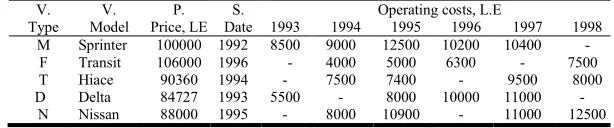
Table 1. Vehicles (V) type, purchase (P) prices, models, Operating costs of studied vehicles and service (S) date
V. Type
V. Model
P. Price, LE
S. Date
Operating costs, L.E
1993 1994 1995 1996 1997 1998 M Sprinter 100000 1992 8500 9000 12500 10200 10400 -
F Transit 106000 1996 - 4000 5000 6300 - 7500
T Hiace 90360 1994 - 7500 7400 - 9500 8000
D Delta 84727 1993 5500 - 8000 10000 11000 -
Third Year
Step 1: C3=1.15SV2 =72482 L. E
Step 2: D*3=0.25C3 =18120 L. E.
Step 3: SV3=0.75 C3 =54361 L. E.
Step 4: O3 from Table 1 =8000 L. E
Step 5: TOC2 =O3 + D*3 =26120 L. E
Step 6: ∑TOC n/n =
3 3 2
1 TOC TOC
TOC = 27996 L.E….etc
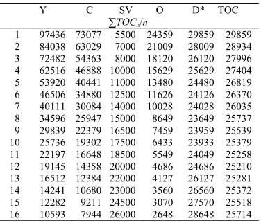
(Table 2 show the calculation of D, SV, O, TOC and ∑TOC
[image:3.612.326.539.60.161.2]n/n from year 4 to year 16).
Table 2. Turning Point of vehicle type D
Y C SV O D* TOC ∑TOCn/n
1 97436 73077 5500 24359 29859 29859 2 84038 63029 7000 21009 28009 28934 3 72482 54363 8000 18120 26120 27996 4 62516 46888 10000 15629 25629 27404 5 53920 40441 11000 13480 24480 26819 6 46506 34880 12500 11626 24126 26370 7 40111 30084 14000 10028 24028 26035 8 34596 25947 15000 8649 23649 25737 9 29839 22379 16500 7459 23959 25539 10 25736 19302 17500 6433 23933 25379 11 22197 16648 18500 5549 24049 25258 12 19145 14358 20000 4686 24686 25210 13 16512 12384 22000 4127 26127 25281 14 14241 10680 23000 3560 26560 25372 15 12282 9211 24500 3070 27570 25518 16 10593 7944 26000 2648 28648 25714
Vehicles Total Operating Cost
Figures 1-5 show both actual TOC for the five vehicles, taken from the ministry of healthy (marked points) and predicted TOC from the best fit for the actual values, to cover the 18 years study range.
[image:3.612.86.274.199.360.2]Figure 1. Influence of vehicle age on actual and predicted TOC, for vehicle type D
Figure 2. Influence of vehicle age on actual and predicted TOC, for vehicle type F
Figure 3. Influence of vehicle age on actual and predicted TOC, for vehicle type T
[image:3.612.69.287.451.702.2]Figure 4. Influence of vehicle age on actual and predicted TOC, for vehicle type N
Figure 5. Influence of vehicle age on actual and predicted TOC, for vehicle type M
Vehicles Scrap Values (SV)
Figures 6-9 show SV for different types vehicles (F, N, T and M), while values of SV for vehicle type D is clear in the Table 2.
0 37500 75000 112500
0 3 6 9 12 15 18
Vehicle type age (F), year
S
V,
L
.E.
Figure 6. Influence of vehicle age on SV for type F
Average Accumulative Operating Cost (∑TOCn/n)
Turning of ∑TOCn/n from decrease to increase considers the economical service years (ESY). It is 12 years for D type (Table 2). By applying the model on the rest of vehicles, as
Vehicle type D 0
10000 20000 30000
0 3 6 9 12 15 18
T
OC,
L
.E.
Vehicle age, year
Vehicle type F 0
10000 20000 30000
0 3 6 9 12 15 18
TO
C,
L
. E
.
Vehicle age, year
Vehicle type T 0
10000 20000 30000
0 3 6 9 12 15 18
T
OC,
L
.E.
Vehicle age, year
Vehicle type N 0
10000 20000 30000
0 3 6 9 12 15 18
T
OC,
L
.E.
Vehicle age, year
Vehicle type M 0
10000 20000 30000
0 3 6 9 12 15 18
T
OC,
L
.E
.
[image:3.612.72.288.454.553.2] [image:3.612.71.287.592.699.2]shown in Figures 10-13, ESY for F is 9, both T and N has the same ESY of D type (12 years), while M is 15 years.
0 37500 75000 112500
0 3 6 9 12 15 18
Vehicle type age (T), year
SV,
L
[image:4.612.325.541.57.142.2].E.
Figure 7. Influence of vehicle age on SV for type T
0 37500 75000 112500
0 3 6 9 12 15 18
Vehicle type age (N), year
S
V
,
L
.E
[image:4.612.78.286.90.171.2].
Figure 8. Influence of vehicle age on SV for type N
0 37500 75000 112500
0 3 6 9 12 15 18
Vehicle type age (M), year
S
V,
[image:4.612.323.539.195.279.2]L.E.
Figure 9. Influence of vehicle age on SV for type M
21000 27000 33000 39000
0 3 6 9 12 15 18
Vehicle type F, Year
∑
TO
Cn
/n
,
L.E
[image:4.612.78.285.225.312.2].
Figure 10. Vehicle age and ∑TOC n/n for type F
21000 27000 33000 39000
0 3 6 9 12 15 18
Vehicle type T, Year
∑
TOCn/n, L. E.
Figure 11. Vehicle age on ∑TOC n/n for type T
21000 27000 33000 39000
0 3 6 9 12 15 18
Vehicle type N, Year
∑
T
OC
n
/n
,
L.
[image:4.612.77.285.364.445.2]E.
Figure 12. Vehicle age and ∑TOC n/n for type N
21000 27000 33000 39000
0 3 6 9 12 15 18
Vehicle type M, Year
∑
T
O
Cn
/n
,
L
.
E
[image:4.612.329.540.399.505.2].
Figure 13. Vehicle age and ∑TOC n/n for type M
RESULTS
ESY Results
Vehicle type M has 15 years ESY, whereas F has 9 and the other types lie between the both (Figure 14).
0 4 8 12 16
M N T D F
Vehicle type
E
S
Y
Figure 14. Vehicle type and ESY
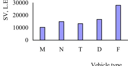
SV Results
Vehicle type M has the lowest value of SV, at its ESY, relative to the others, whereas F has the largest value, the other types lie between the both (Figure 15).
0 10000 20000 30000
M N T D F
Vehicle type
S
V,
L
.E
.
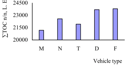
[image:4.612.70.288.489.575.2] [image:4.612.330.541.609.718.2] [image:4.612.68.288.610.699.2]∑TOCn/n Results
Vehicle type T, has the minimum value of ∑TOCn/n relative to the other microbuses, whereas the vehicle type D has the largest value, other types of vehicles lie between them (Figure 16).
20000 21500 23000 24500
M N T D F
Vehicle type
∑
T
O
C n/
n
, L.
E
[image:5.612.70.291.134.247.2].
Figure 16. Vehicle type and ∑TOC n/n
CONCLUSIONS
Three different conclusions on replacement decision-making
listed below.
(1) The best time to get rid of one vehicle is not necessarily the best time to get rid of the other, of the same age and type. (2) The replacement decision is part of a wider problem involving many factors other than depreciation and maintenance costs, such as composition of the vehicle fleet, age profile, interest rates... etc.
(3) The model was formulated on the data of ambulance vehicles, so the study results may change if the same fleet is used in other application.
ACKNOWLEDGMENTS
The author would like to thank the ministry members of health in Egypt, that kindly provided the data required for this study.
REFERENCES
Azrulhisham, E. A, Y. M. Asri, A. W. Dzuraidah, and A. H. Fahmi. 2010. Application of Pearson Parametric Distribution Model in Fatigue Life Reliability Evaluation, World Academy of science, Engineering and Technology.
Berg, P. 1995. The Marginal Cost Analysis and its Application to Repair and Replacement Policies, European Journal of Operational Research, Vol. 82.
Cleroux, R, and C. Tuquin. 1979. The Age Replacement Problem with Minimal Repair and Random Repair Costs, Operation Research, Vol. 27.
Christ, A. C., and W. Goodbody. 1980. Equipment Replacement in an unsteady economy, Journal of the operational Research Society, Vol. 31.
Eilon, S., R. King, and E. Hutchinson. 1996. A Study in Equipment Replacement, Operation Research.
Hastings, N. A., 1969. The Repair Limit Replacement Method, Operational Research Quarterly.
Hyung, K., A. Gregory, and C. James. 2003. Life Cycle Optimization of Automobile Replacement; Model and Application, Center for Sustainable Systems, School of Natural Resources and Environment, University of Michigan.
Jhang, A. 1969. Study of The Optimal Used Period and Number of Minimal Repairs Of a Repairable Product After the Warranty Expires, Int J Syst Sci.
Kobbacy, K, and S. Nicol. 1994. Sensitivity Analysis of Rent Replacement Models, Int. J. Production Economics, Vol. 36, pp. 267-279.
Mahon, B. H., and R. J. Bailey. 1975. A Proposed Improved Replacement Policy for Army Vehicles, Operational Research Quarterly, Vol. 26.
Miguel, A., Jesse, and W. Feng. 2011. Economic and Environmental Optimization of Vehicle Fleets; A Case Study of the Impacts of Policy, Market, Utilization, and Technological Factors, First Submission, Board.
Rai, B., and N. Singh. 2003. Hazard Rate Estimation From Incomplete And Unclean Warranty Data, Reliabil Eng Syst Saf.
Rai, B., and N. Singh. 2004. Modeling and Analysis of Automobile Warranty Data in Presence of Bias Due to Customer-Rush Near Warranty Expiration Limit, Reliabil Eng Syst Saf.
Pillay, A. 2001. Formal Safety Assessment of Fishing Vessels, PhD thesis, Liverpool John Moores University.