Signal Analysis of the Climate: Correlation, Delay and Feedback

ISSN Online: 2327-7203 ISSN Print: 2327-7211

DOI: 10.4236/jdaip.2018.62003 May 17, 2018 30 Journal of Data Analysis and Information Processing

Signal Analysis of the Climate: Correlation,

Delay and Feedback

Peter Stallinga

University of the Algarve, Faro, Portugal

Abstract

One of the ingredients of anthropogenic global warming is the existence of a large correlation between carbon dioxide concentrations in the atmosphere and the temperature. In this work we analyze the original time-series data that led to the new wave of climate research and test the two hypotheses that might explain this correlation, namely the (more commonly accepted and well-known) greenhouse effect (GHE) and the less-known Henry’s Law (HL). This is done by using the correlation and the temporal features of the data. Our conclusion is that of the two hypotheses the greenhouse effect is less like-ly, whereas the Henry’s Law hypothesis can easily explain all effects. First the proportionality constant in the correlation is correct for HL and is about two orders of magnitude wrong for GHE. Moreover, GHE cannot readily explain the concurring methane signals observed. On the temporal scale, we see that GHE has difficulty in the apparent negative time lag between cause and effect, whereas in HL this is of correct sign and magnitude, since it is outgasing of gases from oceans. Introducing feedback into the GHE model can overcome some of these problems, but it introduces highly instable and chaotic behavior in the system, something that is not observed. The HL model does not need feedback.

Keywords

Climate, Temporal Series Analysis, Feedback, Correlations, Hypothesis Testing

1. Introduction

Society is threatened by catastrophic climate changes. Scenarios are given in which temperatures will rise significantly and sea levels will rise causing floods that make coastal areas basically uninhabitable. The source of the climate

How to cite this paper: Stallinga, P. (2018) Signal Analysis of the Climate: Correlation, Delay and Feedback. Journal of Data Analysis and Information Processing, 6, 30-45.

https://doi.org/10.4236/jdaip.2018.62003

Received: March 9, 2018 Accepted: May 14, 2018 Published: May 17, 2018

Copyright © 2018 by author and Scientific Research Publishing Inc. This work is licensed under the Creative Commons Attribution International License (CC BY 4.0).

http://creativecommons.org/licenses/by/4.0/

DOI: 10.4236/jdaip.2018.62003 31 Journal of Data Analysis and Information Processing changes is assumed to be the carbon dioxide that is injected into the atmosphere by burning of fossil fuels and which acts as a greenhouse gas. It blocks outward radiation that otherwise might cool the planet.

We have to take a step back and place this idea in a historic perspective. A politician’s job is to unite people and problems, real, merely imagined or even created, which can be used for that purpose. As the Club of Rome wrote in their report The First Global Revolution,‘‘In searching for a common enemy against whom we can unite, we came up with the idea that pollution, the threat of global warming, water shortages, famine and the like, would fit the bill’’ [1]. Problems serve as a means to a political cause rather than politics as a way to solve them. This is an unfortunate reality. Yet, there was thus a need, as shown by political think-tanks, to prove the ideas of global warming.

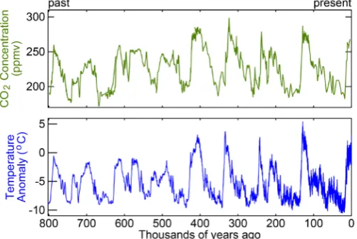
Evidence for the model of global warming through greenhouse gases was soon found in ice core drillings, where a strong correlation between CO2 concentrations found in the air bubbles trapped in it and the temperature (measured via oxygen isotope ratios found in similar ice core drillings). Former vice president of the United States Al Gore, in his documentary An Inconvenient Truth, presented us this convincing data that the earth is warming up and that the carbon dioxide is responsible for it, see Figure 1. The movie landed him a Nobel Prize for Peace and started a new wave in politics and subsequently a wave in climate research, paid for by the politics that convinced us of the urgency. The movie of Al Gore was very convincing. Thus having achieved the first part of the agenda, a politi-cal program was started. One of the items of the program was deviate attention from facts, to never look back at the data or the model, so that attention could be focused on solutions, i.e., mounting political structures such as the Intergo-vernmental Panel on Climate Change (IPCC). “To help address the chaotic na-ture of the climate change discourse in the UK today, interested agencies now need to treat the argument as having been won, at least for popular communica-tions. This means simply behaving as if climate change exists and is real, and that individual actions are effective. The ‘facts’ need to be treated as being so taken-for-granted that they need not be spoken’’ [2]. The subject is taken fully out of the realm of science and placed into the political arena. Each and every report of the IPCC is based on the workflow of starting with an outline of the conclusions—‘‘IPCC approves outline”—and then nominating experts who can help find corroborating data, as they themselves write in their reports.

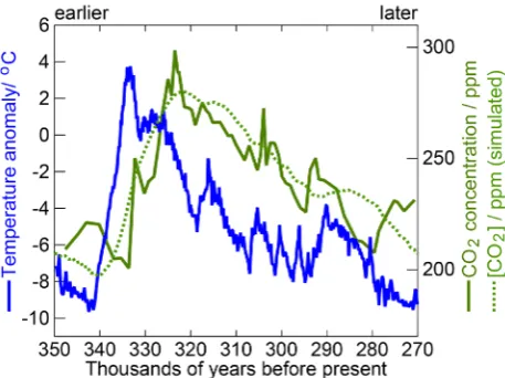
DOI: 10.4236/jdaip.2018.62003 32 Journal of Data Analysis and Information Processing Figure 1. Original data of Al Gore showing the correlation of CO2

(top) and temperature (bottom) as measured by ice core drillings.

presented by Al Gore. Not because we have a hidden political agenda or defend oil-industry—this research was paid by no one—but because we think that so-ciety deserves to know if global warming is really man-made or not. We present here part of our study. There is more going on than simple correlations, as we will show. We will also present an alternative (and older) explanation for the correlation, namely Henry’s Law and check simultaneously if this can stand up to scrutiny.

2. Results and Discussion

2.1. Correlation

Figure 1 shows the entire time series of both CO2 concentration (henceforward abbreviated with [CO2]) in the atmosphere and temperature for the last 800 thousand years, and we can indeed see that there is a strong correlation between the two. What immediately strikes us is that the temperature swing is some 10 degrees for only 100-ppm [CO2]-variations; a climate sensitivity of 0.1 K/ppm. What is so remarkable about this is that modern values of [CO2] go beyond 400 pm, a whopping increase of 125 ppm from pre-industrial values (275 ppm in 1700 [3]), and following the narrative of Al Gore, a staggering temperature rise of 13 degrees is expected. In reality, a meager half a degree is observed, one that is moreover still consistent with a CO2-independent linear rise that started be-fore the industrial era. It surprises us that this fact does not get more attention. Reality falls a factor twenty-five below the model. The enigma of the missing temperature rise.

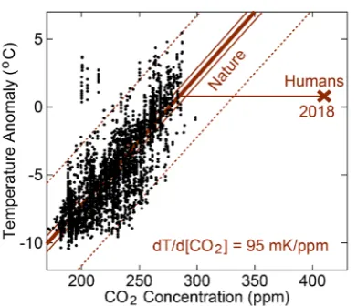
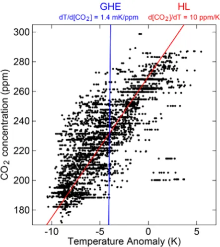
DOI: 10.4236/jdaip.2018.62003 33 Journal of Data Analysis and Information Processing Figure 2. Original data of Al Gore (of Figure 1) presented in a

correlation format. The brown lines labeled “Nature” are a linear-regression fit with confidence interval shown. The contemporary situation of temperature and [CO2] is indicated by

an “X” and labeled “Humans 2018”.

(

)

_[

_]

2

d

observed: 95 mK ppm,

d CO

T _{= (1)}

coefficient of (the fit with confidence intervals is shown in brown and labeled “Nature”). The contemporary CO2 and temperature situation is indicated with an “X” and labeled “Humans 2018”; 410 ppm and +0.8˚C. As can be seen, the tem-perature falls way below the value based on a simple correlation, about 12 degrees; the contemporary situation falls outside the confidence interval. Apparently there is more going on than a simple straightforward correlation between the two in which the CO2 changes are the driving force behind the temperature.

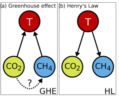
Another interesting and relevant fact that has since the movie of Al Gore been established is that the concentration of methane in the atmosphere also corre-lates with temperature and thus [CO2] ([CH4] not shown here). This seems at first thought to be consistent with a greenhouse-effect hypothesis, since CH4 is a very strong greenhouse agent, thus both change the temperature, see Figure 3(a). However, upon second thought this is very enigmatic. If changes of [CO2] cause temperature variations, and changes of [CH4] do as well, what is the phys-ical effect that correlates [CO2] variations to [CH4] variations? We are opening Pandora’s box asking these questions. Once opened, it cannot be closed, and it has far-reaching consequences. We’d allow for a model in which information passes from [CO2] to [CH4], or vice versa, which implies that temperature can be a cause rather than an effect of things. There, we said it.

DOI: 10.4236/jdaip.2018.62003 34 Journal of Data Analysis and Information Processing Figure 3. Cause and effect relation between atmospheric gases

and the temperature (T). (a) The greenhouse effect of CO2 and

CH4 both influencing the temperature, but how can then CO2

correlate to CH4? (b) Henry’s Law (outgassing of oceans)

where both CO2 and CH4 are caused by temperature changes

and thus also correlate with each other.

both be correct? As a first piece of information we see that the observed correla-tion between [CO2] and [CH4] is very difficult to explain in the GHE hypothesis, whereas it is trivial in the HL hypothesis; Whatever the physical phenomenon that causes the temperature to change the concentration of gases in the atmos-phere, it is very reasonable to think that both CO2 and CH4 are affected simulta-neously.

We now come to the magnitude of the signals. We have seen that the data (Figure 2) point to a correlation of dT/d[CO2] = 95 mK/ppm, or conversely,

(

)

[

]

dT = (2)

be-DOI: 10.4236/jdaip.2018.62003 35 Journal of Data Analysis and Information Processing cause the greenhouse effect is governed by absorption of light, a process that is well studied and follows the Beer-Lambert Law of absorption that is sublinear. To put it in layman’s terms, placing a second curtain over a window that is al-ready closed with a curtain will have as good as no effect. Absorption according to the Beer-Lambert Law is logarithmic and the IR window of the CO2-absorption spectrum is already as good as closed; most heat is radiated outwards in the window of 8 μm to 15 μm where CO2 has no absorption. The ef-fect of CO2 is at around 20 μm [5] and is tiny. If we take this into account, we can find a small GHE correlation coefficient of

(

)

_[

_]

2

d

GHE theory: 1.4 mK ppm,

d CO

T _{= (3)}

i.e., 500 mK for a doubling of CO2 in the atmosphere that has moreover been confirmed by measurements [6]. That is a factor 70 below the observations. How it is possible to still maintain the GHE model we will see in a moment, but first let’s take a look at the alternative HL hypothesis.

Henry’s Law states that the ratio between the partial pressure of a certain gas in an atmosphere above a liquid in which it is also dissolved is constant in equi-librium and this ratio depends on the temperature, and this ratio is called Hen-ry’s Constant. In other words, if the system is in equilibrium and has a certain concentration of CO2 in the oceans and atmosphere above it, when the oceans warm up, the tendency is to outgas the CO2 from the oceans and the concentra-tion in the atmosphere will increase. Al-Anezi and coworkers have studied this effect in more detail in a laboratory setup under various conditions of salinity and pressure, etc. [7]. For synthetic sea-like water at 1 bar, Al-Anezi et al. found a temperature dependence of Henry’s Constant that points to a correlation coef-ficient of about

(

)

[

]

dT = (4)

which is remarkably close to the observed value found in reality. We can now conclude that where science consists of rejecting hypotheses, we must conclude that the greenhouse effect hypothesis is rejected and the Henry’s Law hypothesis still stands. At least the correlation argument used in most discussions point to a cause-and-effect in which temperature is the cause and CO2 the effect. See Fig-ure 4 for a comparison of the GHE model and the HL model with the data.

2.2. Delay

DOI: 10.4236/jdaip.2018.62003 36 Journal of Data Analysis and Information Processing Figure 4. Comparison of the data of Figure 2 with the models of

the greenhouse effect (GHE) of Equation (3) and Henry’s Law (HL) of Equation (4) (with the offset chosen to best fit the data). It is obvious that the HL model cannot be rejected and actually works better than the greenhouse-effect model.

degrees in the (near) future. To study the effects of possible delays, we have to analyze in more detail the exact transient behavior of the two signals, [CO2] and temperature. Plotting the data in the same panel (instead of the rather mislead-ing two-panel format of Figure 1) we see that the CO2 variations seem to be lag-ging behind the temperature variations. Figure 5 shows a zoom in on the data around 300 thousand years before present. We have earlier reported on this re-markable fact [8].

Indermühle and coworkers made a full statistical analysis [9] and find a value of 900 yr for the delay and moreover note that ‘‘This value is roughly in agree-ment with findings by Fischer et al. who reported a time lag of CO2 to the Vos-tok temperature of (600 ± 400) yr during early deglacial changes in the last 3 transitions glacial-interglacial’’ [10]. Fischer and coworkers attribute the delay to the ocean outgassing effects, i.e., Henry’s Law, and even find that at colder times the delay is longer, which is itself consistent with Arrhenius-like behavior of thermally-activated processes, such as most in nature [10].

DOI: 10.4236/jdaip.2018.62003 37 Journal of Data Analysis and Information Processing Figure 5. Zoom in of data of Figure 1 with CO2 and temperature

in the same panel. It shows that the CO2 lags behind the

temperature. The dashed line of CO2 is a convolution of the

temperature data based on a relaxation (time-delay) model. Source: Ref. [8].

First of all, the outgassing and ingassing of carbon dioxide out of and into the oceans and biosphere can easily be determined. As a fortunate side effect of the less-fortunate above-ground nuclear-bomb tests, the residence time of carbon in the atmosphere was accurately determined at some 11 years [11][12], although more recently also shorter times of about 5 - 6 years were found [13]. That means that if the equilibrium of CO2 concentrations is disturbed somehow (for instance by artificially injecting CO2 into the atmosphere by burning of fossil fu-els), it will take some decades to reestablish a new equilibrium. This short resi-dence time has serious implications for the validity of the climate-change model based on the greenhouse effect, even if the greenhouse effect were true and se-riously climate forcing. A residence time of a decade is too short to make CO2 have a serious impact on the climate, the same as the orders-of-magnitude larger greenhouse driver water has no impact on the climate because its residence time is even much shorter, about 9 days [14] although voices were heard that wanted to label water a pollutant as well. To overcome this problem, a new term is coined, namely “adjustment time”, that is estimated to be much longer than the residence time [15], of the order of 80 years, but this naming trick cannot be ex-plained in chemical kinetics (simple reaction kinetics: if most CO2 winds up in the ocean, the residence time and adjustment time are very close). Therefore, we take the two to be the same here.

DOI: 10.4236/jdaip.2018.62003 38 Journal of Data Analysis and Information Processing basically depends on the heat-exchange efficiency between atmosphere and ocean and the mixing rate of the heat in the ocean, both not well established. Yet, we can approach it in a different way, to see if we can get an order of mag-nitude. Imagine that the temperature in the atmosphere is determined by the radiation received from the sun and that for some reason, the radiation balance is disturbed. The advantage is that no, possibly questionable, physics models are involved. We proceed like this: we assume a radiation received from the sun, an albedo (whiteness) of our planet, and a black-body outward radiation of our planet that is required to balance with the incoming radiation to find an equili-brium temperature. We then disturb the radiation to see how that affects the temperature and how fast that will be. Absorbed inward solar radiation is

(

)

2

in π 1 ,

P = R −a W ₍₅₎

with R the radius of our planet, a the albedo (33%) and W the solar radiation constant of 1361 W/m2_{. The outward black-body radiation is}

2 4

out 4π ,

P = R Tσ (6)

with T the temperature at the surface and σ the constant of Stefan and Boltzmann equal to 5.67 × 10−8 _W/(K4_m2_{). In equilibrium the two are equal and} this yields a temperature of T = 251.8 K (note that it does not have an atmos-phere). Now we increase the incoming radiation 1 W/m2_{, either by changing the} albedo or the solar constant. A new temperature will establish that is 69 mK higher. The adjusting of the atmosphere is virtually instantaneous because of its low heat capacity. Now, how long does it take to warm up the oceans 69 mK with this 1 W/m2_{? This 1 W/m}2 _{was through a disk perpendicular to the sunrays.} The spherical earth receives 0.25 W/m2 _{(the factor 4 comes from the ratio of} areas of a disk and a sphere with radius R). 71% of the planet is covered by oceans that are on average 3000 meters deep. The volume of

(

)

2

0.71 4π 3000 m

V = × R × receives an extra _{P=0.71 4× πR}2_×

(

)

heating power. To raise the temperature of 1 liter of water 1 degree takes 4.2 kJ, the initial heating speed is

11

d d d _{2 10 K s,}

d d d

T T U

t U t

−

= ⋅ = × (7)

with U the heat in the ocean, _{d dU T=}

(

)

To establish a new equilibrium thus goes at a time scale of

(

)

(

)

(

)

That is 150 years. Plus the 11 years of adjustment time found before makes a re-sponse time of about 160 years. This is somewhat low compared to the observed 900 years reported by Indermühle [9] and 600 years by Fischer [10], probably because mixing of oceanic layers is required, taking additional time.

be-DOI: 10.4236/jdaip.2018.62003 39 Journal of Data Analysis and Information Processing cause the heat capacity of the atmosphere is not well known. However, we could get a rough estimate by assuming the atmosphere is equal to 10 meters of water (which gives the same pressure as the atmosphere). That is 300 times less than the oceans and we can thus estimate the temperature adjustment time to be half a year. The real value is probably lower, since water has a much higher specific heat (heat per kg) compared to air. We can even do it a little bit more precisely using daily oscillations. As a rough figure, the temperature drops by about 4 de-grees at night in about 8 hours after the sun has set. Assuming that the relaxa-tion upon this step-like solar radiarelaxa-tion is a simple exponential and would finish eventually at close to absolute zero (say 10 kelvin), and starts at 290 K (thus a total amplitude of 280 K): 4 degrees in 8 hours, we solve the equation

(

)

(

)

 

× _− _= −

  (9)

which yields 23 days a value close to the one of 1.2 months one gets when ana-lyzing the periodic yearly oscillations of summer and winter temperatures that lag behind the solar radiation oscillations by about one month [8]. We thus con-clude that the delay between CO2 disturbances and their effect on the tempera-ture has a relation time of some months,

(

)

_τ

(Note the minus sign indicating that temperature lags behind). Indeed, on the total time scale this is virtually instantaneous. In conclusion, the experimental-ly-found delay of some hundreds of years between temperature and [CO2] fits reasonably well with the Henry’s Law, while it even has the wrong sign for the greenhouse-effect hypothesis.

2.3. Feedback and Stability

After having established above what each of the directions of the correlation will be, we can also analyze a system in which both effects occur, both temperature causing [CO2] changes as well as CO2 causing temperature changes. This is what is called feedback. In classical signal analysis the system is imagined to be an amplifier with gain A of which a factor β of the output is added “fed back” to the input. The overall effect on the output (for instance dT) of changes at the input (for instance d[CO2]) can then easily be calculated. For the greenhouse model we get

[

]

d _,

d CO 1

A T

A β

=

− (11)

with the subscript indicating the hypothesis. See Figure 6(a).

Where the gain of the greenhouse effect could roughly be calculated on phys-ical properties and resulted in an estimated value of AGHE =d d COT

[

]

DOI: 10.4236/jdaip.2018.62003 40 Journal of Data Analysis and Information Processing Figure 6. (a) Changes in T, caused by changes in [CO2]

are fed back and cause additional changes in [CO2]. (b)

Changes in [CO2], caused by changes in T are fed back

and cause additional changes in T. (c) A symmetric way of representing feedback. Feedback.

DOI: 10.4236/jdaip.2018.62003 41 Journal of Data Analysis and Information Processing Note that the found value of βGHE makes the denominator in the above for-mula close to zero and such systems (and calculations) are very sensitive; small changes of beta can have huge effects on the response. For instance, a slightly larger βGHE of 0.7132 ppm/mK (about 1% larger) will make the response tenfold. It is moreover highly dubious that nature is this close to the critical value that creates a singularity (at βGHE =1 AGHE =0.7142 ppm mK). Any feedback factor

at or above this critical value will cause an infinite response, dT/d[CO2] = ∞. That is the problem with positive-feedback systems. They have huge gain and are unstable when the so-called “open-loop gain” AGHE GHEβ ≥1. For this reason

the wording ‘‘point of no return’’ is often used; it hints at the instability of the system (simulated). A run-away scenario is built into the simulations. Imagine that the melting of the ice will increase the “open loop gain” just a little, either through βGHE or AGHE. A catastrophe is envisaged.

That while nature is obviously very stable. It recovers daily from huge tem-perature oscillations. Similarly it recovers from yearly periodical seasons (with also periodic modulation of the solar flux caused by the ellipticity of Earth’s or-bit), as well is able to recover from aperiodic fluctuations such as El Niños and La Niñas. This hints at negative feedback (βGHE <0), or small feedback with the

open-loop gain much smaller than unity. Such feedback makes the system stable, with the absence of any criticality. Negative feedback even attenuates the overall gain of the system. As an example, the value of βGHE of −0.70376 ppm/mK above would about halve the overall gain to 0.71 mK/ppm, as Equation (11) easily shows.

On the other hand, the model based on Henry’s Law does not need feedback, let alone critical feedback. The gain of the system is AHL = 10 ppm/K, and a small feedback (which might be the greenhouse effect, thus βHL=AGHE=1.4 mK ppm)

does not change this value appreciably (only about 1%).

[

]

HL HL

d CO

,

d 1

A

T = −A β (12)

See Figure 6(b).

In the above we talked about “gain” since this is classic jargon of the signal processing field. However, gain is only defined if the input and output quantities are in the same domain. In our case we have two different domains, T and [CO2]. A better picture is shown in Figure 6(c). It has two transfer functions

2

CO T

A and T ₂ CO

A modeling the response to changes in [CO2] upon changes of T and changes of T upon changes of [CO2], respectively. Where either one can be seen as “gain” or “feedback”; to translate the circuit in Figure 6(c) to the one in Figure 6(b), we substitute CO2

HL T

A = A and T ₂

HL ACO

β = , and to translate

the circuit in Figure 6(c) to the one in Figure 6(a), we substitute T ₂ GHE CO

A = A

and CO2

GHE AT

elimi-DOI: 10.4236/jdaip.2018.62003 42 Journal of Data Analysis and Information Processing nated the fitting parameter β from the equation—no fitting parameter is left whatsoever—and yet, it fully reproduces the observed data. The inevitable con-clusion is that the temperature variations were the source of the [CO2] variations and not the other way around.

Note that the loop gain equals, 2

(

) (

)

2 CO T

CO T 10.5 ppm K 1.4 mK ppm

A × A = ×

3

1.47 10−

= × _{, and, while positive, this is far away from instability. The climate} system, while chaotic and unpredictable, is stable on the long run.

Feedback analysis can also make statements about the stability as a function of frequency—periodicity of the driving force. The gain and feedback—transfer functions in general—may depend on frequency and a system may start to oscil-late without external driving signals at those frequencies where the open-loop gain is positive and larger than unity. Apart from a loop gain, Aβ also introduces a phase shift, and the two are normally presented in a so-called Nyquist plot. In phasor terminology we define an amplitude and a phase:

( ) ( )

( ) ( )

( )

A ω β ω = A ω β ω iφ , where ω is the (radial) frequency and φ

the phase, and plot the real and imaginary part of this product, see Figure 7. The point of perfect oscillation (open-loop gain unity and phase zero) is called the Barkhausen Criterion (BC). Inside the circle indicating a unity gain, no oscilla-tion takes place, whereas outside it oscillaoscilla-tion can take place if the phase is cor-rect. (Note that an “oscillation” at zero hertz is simply the run-away scenario described before). Figure 7 summarizes this for our models. We saw that a process of Henry’s Law outgassing has a characteristic time of τ = 600 year and such a relaxation process causes an attenuation of the response for higher frequencies as well as a phase shift tending towards −90˚, i.e., one quarter period lagging behind. In the Nyquist plot this is a semicircle (see the zoom in at the bottom left; the bottom of the semicircle occurs at ω=1τ _{), the phase shift} which has been observed [8]. This means that for higher frequencies the system, even though the feedback does not become negative, becomes ever more stable. For the greenhouse effect, the delay of CO2 having effect on the temperature is about a month, as we have discussed above, but other effects that are not simple first-order (relaxation) behavior might make the system enter into the unstable behavior, which is often mentioned in popular press, since it is critically stable; there must then be especially high-frequency oscillations in both temperature and [CO2].

3. Summary and Conclusions

The greenhouse effect cannot explain the experimental data because it does not manage to reproduce the correlation coefficient between temperature variations and carbon-dioxide concentration variations, unless a feedback is added to the system. This feedback factor is then coincidentally very near the critical value, which would turn the climate system marginally stable with real risk for cata-strophic climate scenarios. Moreover, this feedback factor must be really huge;

(

)

HL 10.5 ppm K

DOI: 10.4236/jdaip.2018.62003 43 Journal of Data Analysis and Information Processing Figure 7. Feedback and stability. The open-loop gain of feedback represented in a Nyquist plot. The Henry’s Law system is stable and feedback makes it more stable at higher frequencies (see zoom in at bottom left). The system controlled by the greenhouse effect is marginally stable, but any perturbation can make it unstable, which is not observed in nature that is always recovering easily from disturbances such as seasonal oscillations and El Niño and La Niña events.

for the observed data, there do not seem to be any physical phenomena that might explain such large feedback factors. An outgassing of tundra’s or the al-bedo effect is too small.

What is more, the greenhouse hypothesis does not have an explanation for the simultaneously occurring correlation with methane in the atmosphere. Moreo-ver, the delay between the temperature and the [CO2] variations demonstrate that the temperature cannot be the effect of [CO2] variations but rather must be their cause.

On the other hand, Henry’s Law hypothesis can explain the correlation be-tween temperature and carbon dioxide in the atmosphere flawlessly, both the correlation coefficient, as well as the time delay. Moreover, it also explains the correlation with methane. It does not need any feedback, but adding a green-house effect as feedback to the system does not alter the behavior significantly (only by about 1%).

We therefore come to the conclusions that the model as presented in Figure 8

is correct, where the values of the parameters are based on experimental beha-vior instead of our calculations. It leads in signal analysis to a response function equal to

[

]

( ) (

)

(

)

(

[

]

)

d CO t = 10.5 ppm K ⋅

_∫

This technique was used in a simulation of Figure 5[8].

DOI: 10.4236/jdaip.2018.62003 44 Journal of Data Analysis and Information Processing Figure 8. Final model including an outgassing of oceans

that has an adjustment time of 600 years and a response of 10.5 ppm/K.

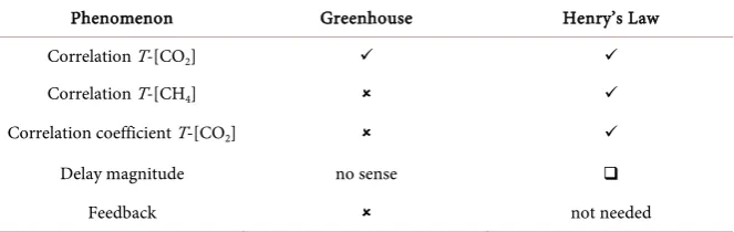
Table 1. Comparison of the two models of greenhouse effect and Henry’s Law describing the observed phenomena. : good. : reasonable. : problematic.

Phenomenon Greenhouse Henry’s Law

Correlation T-[CO2]  

Correlation T-[CH4]  

Correlation coefficient T-[CO2]  

Delay magnitude no sense 

Feedback  not needed

Disclosure of Interests

The author declares not to have any conflict of interests. This research was paid by no grant. It received no funding whatsoever, apart from the salary at the uni-versity where he works. Nor is he member of any climate committees (political or other) or is he linked to companies or NGOs, financially or otherwise. He is not member of any political party or movement. This is an independent work that does not necessarily represent the opinion of his university or of his gov-ernment. The author wishes to thank Prof. Khmelinskii for valuable discussions.

References

[1] King, A. and Schneider, B. (1991) The First Global Revolution. A Report by the Council of the Club of Rome. Orient Longman, Hyderabad, 75.

[2] Ereaut, G. and Segnit, N. (2006) Warm Words: How We Are Telling the Climate Story and Can We Tell It Better? Institute for Public Policy Research, London, Eng-land.

[3] Frank, D.C., et al. (2010) Ensemble reconstruction Constraints on the Global Car-bon Cycle Sensitivity to Climate. Nature, 463, 527-530.

https://doi.org/10.1038/nature08769 [4] Hieb, M. (2007)

http://www.geocraft.com/WVFossils/greenhouse_data.html

[5] Rothman, L.S., et al. (2005) The HITRAN 2004 Molecular Spectroscopic Database. Journal of Quantitative Spectroscopy & Radiative Transfer, 96, 139-204.

https://doi.org/10.1016/j.jqsrt.2004.10.008

[6] Lindzen. R.S. and Choi, Y.-S. (2009) On the Determination of Climate Feedbacks from ERBE Data. Geophysical Research Letters, 36, L16705.

https://doi.org/10.1029/2009GL039628

DOI: 10.4236/jdaip.2018.62003 45 Journal of Data Analysis and Information Processing Seawater at the Conditions Encountered in MSF Desalination Plants. Desalination, 222, 548-571.

[8] Stallinga, P. and Khmelinskii, I. (2014) Application of Signal Analysis to the Cli-mate. International Scholarly Research Notices,2014, Article ID: 161530. https://doi.org/10.1155/2014/161530

[9] Indermühle, A., Monnin, E., Stauffer, B., Stocker, T.F. and Wahlen, M. (2000) At-mospheric CO2 Concentration from 60 to 20 Kyr BP from the Taylor Dome Ice

Core, Antarctica. Geophysical Research Letters, 27, 735-738. https://doi.org/10.1029/1999GL010960

[10] Fischer, H., Wahlen, M., Smith, J., Mastroianni, D. and Deck, B. (1999) Ice Core Records of Atmospheric CO2 around the Last Three Glacial Terminations. Science,

283, 1712-1714.https://doi.org/10.1126/science.283.5408.1712

[11] Nydal, R. and Lovseth, K. (1983) Tracing Bomb 14_{C in the Atmosphere 1962-1980.}

Journal of Geophysical Research, 88, 3621-3642. https://doi.org/10.1029/JC088iC06p03621

[12] Levin, I., et al. (2010) Observations and Modelling of the Global Distribution and Long-Term Trend of Atmospheric 14_CO

2. Tellus, 62, 26-46.

[13] Essenhigh, R.H. (2009) Potential Dependence of Global Warming on the Residence Time (RT) in the Atmosphere of Anthropogenically Sourced Carbon Dioxide. Energy & Fuels, 23, 2773-2784.https://doi.org/10.1021/ef800581r

[14] van der Ent, R.J. and Tuinenburg, O.A. (2016) The Residence Time of Water in the Atmosphere Revisited. Hydrology and Earth System Sciences, 21, 779-790. https://doi.org/10.5194/hess-2016-431

[15] Cawley, G.C. (2011) On the Atmospheric Residence Time of Anthropogenically Sourced Carbon Dioxide. Energy & Fuels, 25, 5503-5513.

https://doi.org/10.1021/ef200914u

[16] Stallinga, P. and Khmelinskii, I. (2014) The Scientific Method in Contemporary (Climate) Research. Energy & Environment, 25, 137-146.