A Fuel-Payload Ratio Based Flight-Segmentation
Benchmark
Kim Kaivanto§∗and Peng Zhang‡
§Lancaster University, Lancaster LA1 4YX, UK ‡Guizhou Minzu University, Guiyang City, PRC 550025
this version: May 8, 2018
Abstract
Airlines and their customers have an interest in determining fuel- and emissions-minimizing flight
segmentation. Starting from K¨uchemann’s Weight Model and the Breguet Range Equation
for cruise-fuel consumption, we build an idealized model of optimal flight segmentation for
maximizing fuel efficiency and minimizing emissions under the assumption that each leg is
operated with an aircraft of segment-length-matching design range. When a multi-leg (≥ 2)
itinerary is most efficient, legs are ideally of equal length. Instrumental to the parsimony of
this flight-segmentation benchmark is a new efficiency metric: Fuel-Payload Ratio (FPR). The
FPR approach has a one-to-one correspondence with the standard microeconomic cost-curves
framework, which avails the standard tools of microeconomic analysis for cost-efficient
design-range determination and optimal flight segmentation. This makes it possible to make direct
comparisons between (i) technically efficient design-range and flight-segmentation solutions and
(ii) their economically efficient counterparts. Even modest fixed-cost components cause the
latter to diverge non-trivially from the former.
Keywords: scheduled passenger air transport, flight segmentation, fuel efficiency, greenhouse
gas emissions, microeconomics
JEL classification: Q54, D62, D03, L93
∗
1 Introduction
Air transportation is caught between two converging fronts. The first is increasing demand for
air transportation, driven by income growth – notably, at a rate faster than income growth itself
– during an era of consistently increasing world Gross Domestic Product (GDP).1 The second
is accelerating anthropogenic climate change, and the consequent need to reduce greenhouse
gas (GHG) emissions drastically in order to avoid global-ecosystem-altering climate change.
Technological innovation and far-reaching policy changes will be required in the medium term
in order to achieve the targets agreed to in the United Nations Framework Convention on Climate
Change (UNFCC COP21).
But in the short run, the GHG footprint of air transportation can be reduced by optimizing
aircraft design-and-deployment decisions within the envelope of current technological
possibil-ity. This builds upon and makes the most of ongoing technological innovation to improve the
efficiency of propulsion technology, improve wing and airframe strength-to-weight ratio by the
introduction composite technology, and improve aerodynamic efficiency by e.g. the introduction
of winglet technology (Cansino and Rom´an, 2017).
Although several methods exist for calculating the GHG emissions of scheduled air transport,
the dominant component common to all methods is mission fuel (see e.g. Kaivanto and Zhang,
2017). Nevertheless mission fuel is not the only determinant of GHG emissions. Non-fuel-based
measures – such as lowering the cruise altitude2and rerouting aircraft trajectories in real time to
mitigate persistent contrail formation – are potentially important complementary components
of emissions-reduction policy packages (Dallara and Kroo, 2011; Campbell et al., 2013). In the
present paper however, the focus is on fuel and the possibilities for economizing on fuel burn
through optimal flight segmentation.
Whereas route-structure variables are among the many that airlines and air-transport
au-thorities typically optimize jointly (e.g. Dumas et al., 2009; Li et al., 2010; Pita et al., 2014;
Dalmau and Prats, 2015), here we tackle the flight-segmentation aspect of route structure in
1
In the post-1970s era, GDP has consistently grown, with the exception of one year in which the world economy absorbed the fallout from the financial crisis (2009). The empirical income elasticity of demand for air transportation services is widely documented to be greater than 1: for every 1% increase in income (i.e. GDP), demand for air transport increases bymorethan 1% (IATA, 2008; Chi and Baek, 2012; Gallet and Doucouliagos, 2014).
2
isolation. By doing so, we abstract from the numerous variables and considerations for which
fuel burn and GHG emissions are traded off in joint optimization exercises. In this sense, we
investigate a pure – and therefore idealized – fuel- and emissions-focused flight-segmentation
benchmark.3
This problem definition is not without precursors in the literature. Yutko and Hansman
(2011) report4 the frequencies of operations (legs flown) by all US carriers at different fractions
of design range (R1), separately for narrow-body aircraft, wide-body aircraft, an regional jets.5
The mean of narrow-body aircraft operations was at 41% ofR1; the mean of wide-body aircraft
operations was at 61% of R1; and the mean of regional-jet aircraft operations was at 39% of
R1. Virtually all passenger air-transport movements are therefore sacrificing fuel and emissions
efficiency by being operated with aircraft of much greater design range. Zeinali and Rutherford
(2010) also document this “inferior environmental performance during actual operation” and
suggest that it may be the result of a ‘one-size-fits-all’ approach in which aircraft are sized to
meet extreme missions – presumably to offer the greatest possible scope for flexible deployment
– rather than to meet representative payload-range missions. Thus, modern jet aircraft are
over-sized and consequently less efficient in operation than current technology is capable of delivering.
Accordingly Zeinali and Rutherford (2010) identify “aircraft rightsizing” as a means of realizing
efficiency improvements and emissions reductions – which they identify as a key challenge for
the International Civil Aviation Organization (ICAO).
In turn Perez and Jansen (2014) advocate coupled design optimization, in which the aircraft’s
design configuration is optimized specifically for taking advantage of Intermediate Stop
Opera-tions (ISOs). The question of how ISO routes should be designed to maximize fuel and GHG
efficiency is also broached by Green (2002), but his recommendations are couched in preliminary
and suggestive language.6 Poll (2011) revisits this question, and finds that significant fuel- and
GHG-related savings are only available for distances greater than 5,500 km. Martinez-Val et al.
3
Even though there may currently be practical impediments to full implementation of the present idealized flight-segmentation method, shifts toward this benchmark yield efficiency improvements. This is similar in spirit to Dalmau and Prats’ (2015) proposal, also published in TRD, for achieving fuel and time savings by flying continuous-cruise climbs, rather than the constant-cruise-altitude flight levels currently operated under Air Traffic Control (ATC) direction.
4
in their analysis of 2006 Bureau of Transportation Statistics (BTS) Form 41 T-100 data 5in their Figures 16, 17 and 18, respectively.
6
(2013) and Langhans et al. (2013) also begin with this question, but find that there is a tension
between the engineering objectives of achieving fuel savings and reducing environmental impact,
on the one hand, and economic cost efficiency, on the other hand. Our investigation aims to
synthesize and deepen the aforementioned results parsimoniously.
This paper’s novel contributions range across three dimensions.
First, the Fuel-Payload Ratio (FPR) efficiency measure – although derived from the same set
of equations Green (2002, 2006) employs – has a direct interpretation in the standard
microeco-nomic framework as the lower envelope of Total Variable Input (TVI) curves, which avails all of
the standard microeconomic analysis tools. Using this microeconomic framework, we illustrate
how Fixed Costs affect Average-Total-Cost-minimizing design range, thereby contributing to our
understanding of the empirical disparity between the design ranges of aircraft purchases (and
stock thereby created) based on economic drivers and the design ranges of aircraft purchases
(and associated stock created) if they were guided purely by technical (fuel, GHG) efficiency.
Second, the present study of flight segmentation aims to sharpen Green’s (2002) somewhat
vague suggestions concerning efficiency-maximizing stage length. Hence the present study is
distinct from, but responds to, complements, and sharpens Green (2002). The advantage of the
FPR-based approach is that its mathematical form provides straightforward answers to these
types of questions.
Third, the sensitivity analysis reported in this study investigates the effects of pertubations
in (i) the ‘lost-fuel’ fractionλof take-off weight that is consumed during takeoff, climb-to-cruise
altitude and acceleration-to-cruise speed, and (ii) the range-performance parameter X, which
is a composite of propulsive efficiency and aerodynamic efficiency. In contrast, Green’s (2002)
sensitivity analysis studies the effects of pertubations in structural constants of proportionality
pertaining to maximum take-off weight and payload. Hence the present study is distinct from,
but complements Green (2002).
In Section 2 we investigate the impact of design range on commercial air transport fuel
effi-ciency by developing a model drawing on K¨uchemann’s (1978) Weight Model and the Breguet
Range Equation for cruise fuel consumption. These two equation families complement each
other. K¨uchemann’s (1978) Weight Model is a standard if not classic7 decomposition of aircraft
take-off weight into components that roughly correspond to airframe empty weight, payload,
en-gines, and mission fuel. The Breguet Range Equation in turn allows cruise range to be expressed
as a function of (i) aircraft initial weight at take-off, (ii) aircraft ‘final weight’ upon landing, after
mission fuel has been consumed, and (iii) range-performance parameters capturing the calorific
energy content of the fuel, the propulsive efficiency of the engine, and the aircraft design’s
lift-to-drag ratio. Using these euqations Green (2002) derived the Payload Fuel Efficiency (PFE)
metric, defined as the product of range and the ratio of the weight of payload to mission fuel. We
build on this in Section 3 to introduce a new efficiency metric, the Fuel-Payload Ratio (FPR),
which captures the technical relationship between mission fuel burn and payload transported to
design range. With the aid of this FPR metric, identification of optimal design range (Section
3.2), as well as optimal thresholds for 1-, 2-, and 3-segment flights (Section 3.3), is
straightfor-ward. Furthermore, 1/FPR may be understood as a short-run production function in a standard
microeconomic sense, from which it follows that the standard short-run curves – marginal and
average product, variable cost and total cost, marginal cost, average variable cost and average
total cost – may also be derived straightforwardly. This makes it possible to undertake
eco-nomic optimization of the design-range decision parsimoniously, without abstracting from any
of the the engineering information contained in Green’s (2002) PFE metric. We conclude with a
sensitivity analysis (Section 4) that complements rather than replicates the sensitivity analysis
undertaken in Green (2002).
2 Flight-range design for fuel efficiency
In the past two decades the literature on optimal aircraft design for environmental impact
reduction has become an important stream within air transport research (Lee at al., 2001; Green,
2009; Dallara, 2011; Dallara and Kroo, 2011). Specifically, the relationship between design range
and fuel efficiency has drawn particular attention (Green, 2002, 2006). However, most studies in
the literature opt for numerical illustration of theoretical predictions, and therefore an analytical
treatment of this topic is often absent. In this section we present a model composed of
well-known results in this literature, and we apply this analytical model to the problem of fuel- and
2.1 Nomenclature
c1 structural constant of proportionality related to maximum take-off weight
c2 structural constant of proportionality related to payload
H calorific value of fuel (energy per unit mass)
OEW operating empty weight
L/D lift-to-drag ratio at cruise
PFE payload fuel efficiency
FPR fuel-payload ratio
R design range
WE weight of engine
WMF weight of mission fuel
WP weight of payload
WTO aircraft weight at takeoff
Winitial aircraft weight at the beginning of cruise
Wfinal aircraft weight at the end of cruise
X aircraft range parameter
λ the fraction of aircraft weight at takeoff as lost fuel
η overall propulsive efficiency
2.2 Theory
K¨uchemann (1978) proposes a basic decomposition of aircraft weight at take-off, which consists
of four components.
WTO =c1WTO+c2WP+WE+WMF (1)
The first term captures necessary mass elements of the aircraft. The second term represents
payload and the fittings/furnishings that vary in proportion to payload. The third term is the
fixed weight of engines. The last term is the weight of mission fuel.
Green (2002) simplifies this model further by assuming that engine weight is also proportional
to the total weight at takeoff and can be incorporated into c1, resulting in the following
As in Green (2002), we introduce the Breguet Range Equation as
R=Xln
Winitial Wfinal
(3)
where R represents the design range and X represents a range-performance parameter defined
as
X =HηL
D (4)
whereH is the calorific value of the fuel,η is the overall propulsion efficiency of the engine and
L
D is the lift-to-drag ratio of the aircraft at cruising speed.
Assume that ‘lost fuel’ – defined as fuel consumed during takeoff, climb-to-cruise altitude
and acceleration-to-cruise speed (Torenbeek, 1997) – weighs a fraction λ of aircraft weight at
takeoff (λWTO). Then we have
Winitial = (1−λ)WTO (5)
Wfinal = Winitial−(WMF−λWTO) (6)
whereWMF represents the total mission fuel weight. In Green (2002),λis assumed to be 2.2%,
while in the present study we take a more general approach and investigate the impact of the
parameter value. Substituting equations (5) and (6) into the Breguet range equation yields
WMF=WTO 1−
1−λ
exp XR !
(7)
By combining this with equation (2) and rearranging, we have the mission fuel weight as a
function of range and payload weight.
WMF=
1 1−λexp
R X −1 c2
1− 1
1−λexp R X
c1
WP (8)
The Greener by Design Technology Sub Group (2002) characterizes fuel efficiency with
‘Pay-load Fuel Efficiency’ (PFE) defined as the ratio of the product of range and pay‘Pay-load to mission
fuel:
PFE = R·WP
WMF
Combining equations (8) and (9) yields
PFE = R(1−λ−exp R X
c1)
c2(exp XR
−1 +λ) (10)
The efficiency maximization problem can be expressed as
max
R PFE s.t. R≥0 .
The derivative of PFE with respect to design range (R) is a nonlinear function, and therefore
optimal R cannot be solved for easily in closed form. We follow Green (2002) in employing a
numerical approach to illustrating the properties of this maximization problem, and conduct a
sensitivity analysis in Section 4.
2.3 Numerical illustration
In order to illustrate how PFE varies with design range, parameter values need to be determined
for X, λ, c1 and c2. Using Fielding’s (1999) data, Green (2002, 2006) estimates c2 to be 2.0.
Green (2006) revisits the estimation ofc1 in light of Nangia (2006), and using Fielding’s (1999)
data Green (2006) estimates c1 to be 0.345.8 We also follow Green (2002, 2006) in employing
the aircraft range parameter X = 30,580km and the lost-fuel fraction λ= 2.2%. Substituting
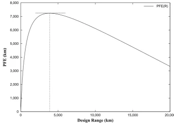
these parameter values into equation (10) and plotting PFE against range R, we obtain Figure
1.
Figure 1 verifies Green’s (2006) finding that efficiency measured by PFE is a concave function
of design range and reaches maximum when design range is in the region of 3,872km for a typical
wide-body swept-wing kerosene-fueled aircraft. When design range is shorter than 3,872km, a
large fraction of mission fuel is consumed in the take-off and climb stage, leading to low efficiency.
When design range exceeds 3,872km, a large mass of mission fuel will be carried for a long
distance before combustion, leading to decreasing efficiency as design range is pushed beyond
3,872km.
8These values forc
Figure 1: Payload fuel efficiency against design range: Wide-body swept-wing kerosene-fueled aircraft.
0 1,000 2,000 3,000 4,000 5,000 6,000 7,000 8,000
0 5,000 10,000 15,000 20,000
PFE (km)
Design Range (km)
PFE(R)
3 Optimal flight segmentation – a new approach
3.1 Fuel-Payload Ratio
We develop a new approach to the finding in Section 2 that yields new insight into the theory,
particularly with regard to economizing on GHG emissions achieved through optimal flight
segmentation. Instead of focusing on Payload Fuel Efficiency PFE), we propose a new metric,
the Fuel-Payload Ratio (FPR), defined as the ratio of mission fuel weight to payload weight.
Following the above-developed model based on K¨uchemann’s Weight Model and the Breguet
Range Equation, FPR can be written as
FPRR =
WMF WP
R
= exp
R X
−1 +λ
1−λ−exp XRc1
·c2 (11)
This ratio measures the mission fuel required to deliver a one-unit payload to a specified range,
using an ideal aircraft with matching design range. We will show that, compared to efficiency
measured by the PFE factor introduced in Section 2, a re-description of the same model using
this ratio brings new insight regarding fuel efficiency and GHG-emissions reduction, in particular
3.2 Numerical illustration
In this numerical example, we continue to employ the parameter values introduced above in
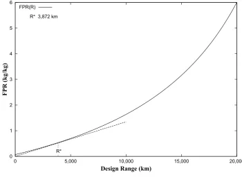
Section 2.3.9 Substituting these parameter values into equation (11) and plotting FPR against
[image:10.595.120.471.208.464.2]range R, we obtain Figure 2.
Figure 2: Fuel-Payload Ratio against design range: Wide-body swept-wing kerosene-fueled air-craft.
0 1 2 3 4 5 6
0 5,000 10,000 15,000 20,000
R* 3,872 km
FPR (kg/kg)
Design Range (km)
FPR(R)
R* R*
Several observations may be made regarding FPR.
Finding 3.1 (Mission fuel increases with R, at an accelerating rate). For a typical
swept-wing kerosene-fueled aircraft, FPR is a convex function of design range. The total weight
of mission fuel required to deliver a one-unit payload to the design range is increasing in design
range at an accelerating rate. Furthermore, this increasing rate (f00 > 0) is itself increasing
(f000 >0). This is due to the fact that as design range increases, more fuel will be carried for a
longer distance before combustion, creating a self-reinforcing feedback loop in the mission fuel
required.
Finding 3.2 (min FPR/km design range = R∗). Figure 2 also contains information
re-garding Payload Fuel Efficiency from Figure 1. If we draw a line segment from the origin to any
9
point along the FPR curve, the slope of this line segment is equal to the inverse of the Payload
Fuel Efficiency, i.e. 1/PFE. The FPR curve’s vertical intercept is at (0,0.070).10 As the line
segment’s end point on the FPR curve moves to the right from the vertical intercept, the slope
first decreases, and then eventually increases. The lowest-slope line segment from the origin
is tangent to the curve at the abscissa coordinate associated with a design range of 3,872km
(rounded to the nearest km). At this design range
FPR
R =
dFPR
dR (12)
and
arg minFPR
R = arg min
dFPR
dR =R
∗ (13)
This is the design range at which minimum FPR/km is achieved.
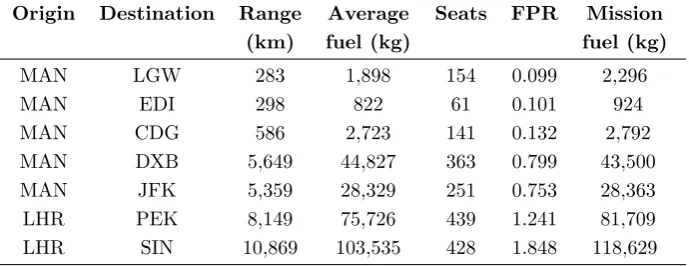
Finding 3.3 (FPR-based mission fuel is validated by ICAO data). The FPR curve in
Figure 2 fits empirical data well. Table 1 contains ICAO data on flight range, average
mission-fuel consumption and average number of seats (columns 3–5).11 Using these data, FPR values
are calculated from Figure 2 and total mission fuel is calculated (rounded to the nearest integer)
assuming a 150kg payload for each average seat. The departure and destination airports are
chosen so that the data contain short-, medium-, long- and ultra-long-haul flights. We can see
that the calculated mission fuel consumption (column 7) fits ICAO average fuel data (column
4) quite well, especially for medium and long range flights. This suggests that the FPR method
in Figure 2 provides a reliable method for estimating mission fuel consumption, especially for
medium- and long-haul flights.
Finding 3.4 (Standard microeconomic interpretation). In a microeconomic context the FPR curve in Figure 2 corresponds to the lower envelope of Total Variable Input (TVI) curves,
where each TVIR0 curve is obtained as the locus of FPR when flying an aircraft optimized for
10
The reason for positive mission fuel at zero range comes as a result of the simplified assumption that fuel for take-off, climb and manoeuvre stand as 2.2% of total weight of the aircraft at take-off, even when range decreases to zero. Zero and very small ranges are included mainly as part of a complete mathematical description and graphic demonstration, but it is understood that they lack meaningful interpretation in practice.
11
Table 1: Average fuel burn ICAO vs. FPR-based mission-fuel calculation
Origin Destination Range Average Seats FPR Mission
(km) fuel (kg) fuel (kg)
MAN LGW 283 1,898 154 0.099 2,296 MAN EDI 298 822 61 0.101 924 MAN CDG 586 2,723 141 0.132 2,792 MAN DXB 5,649 44,827 363 0.799 43,500 MAN JFK 5,359 28,329 251 0.753 28,363 LHR PEK 8,149 75,726 439 1.241 81,709 LHR SIN 10,869 103,535 428 1.848 118,629
design range R0 on legs of length [0,20,000].12 Transposing the axes yields the
R=f(FPR) (14)
curve, which has the microeconomic interpretation of the upper envelope of short-run
‘design-range’ production functions: the horizontal axis indicates the variable input (kg of mission fuel
per kg of payload) and the vertical axis indicates the design range attained. Implicit inf(·) is
the current level of technology that embodies what could be stated explicitly as fixed capitalK.
Placing FPR within a microeconomic framework leads to insights that are typically not
available within a purely technical engineering analysis. For instance, FPRR=
WMF
WP
may be
re-expressed in monetary-unit terms by multiplying equation (11) by the price of kerosene ($/kg)
– i.e. the vertical axis of Figure 2 may be re-indexed by multiplying by the price of kerosene,
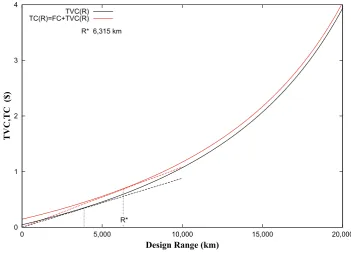
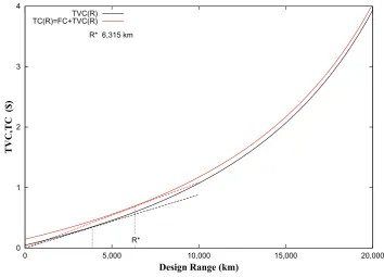
which at the time of writing is 654.8 $/mt or 0.6548 $/kg (see Figure 3).13 On this cost scale,
the FPR becomes the lower envelope of Total Variable Cost (TVC) curves. This opens up the
possibility of investigating the effect of changes in Fixed Costs (FC) on cost-efficient choice of
design range – regardless of whether those Fixed Costs arise from engineering, regulatory (e.g.
environmental regulations), safety and service, or other business-environment considerations.
Figure 3 illustrates how a 10¢ increase in Fixed Cost14increases Average-Total-Cost-minimizing
design range by over 2,400 km.
12
Every range-R0-optimized design has FPR(R0) values that lie on or above the FRP curve pictured in Figure
2. 13
Jet fuel price obtained from The International Air Transport Association (IATA) Jet Fuel Price Monitor on 30 March 2018. http://www.iata.org/publications/economics/fuel-monitor/Pages/index.aspx
Figure 3: Total Variable Cost (TVC) and Total Cost (TC) envelopes against design range, where the Fixed Cost (FC) component of TC is 10¢ per payload kg.
0 1 2 3 4
0 5,000 10,000 15,000 20,000
R* 6,315 km
TVC,TC
($)
Design Range (km)
TVC(R) TC(R)=FC+TVC(R)
R* R*
This microeconomic analysis of the effect of Fixed Costs carries two types of implications.
First, it goes some way to explaining why the stock of aircraft operated on short- and
medium-length segments are ‘oversized’ in terms of design range: economic considerations rather than
purely technical fuel- and GHG-effiiciency considerations weigh heavily in the aircraft purchase
decision. Second, it shows the unintended consequences of introducing regulations – whether
motivated by environmental-protection concerns or not – that increase payload Fixed Cost.
Finally and perhaps most importantly, FPR brings new insight to fuel- and
emissions-efficiency by providing guidance on optimal flight segmentation. We develop this in the next
section.
3.3 Optimal route-segmentation benchmark
Compared to expressing efficiency through Payload Fuel Efficiency, the new representation in
Figure 2 emphasizes mission fuel and GHG emissions directly. This advantage becomes
partic-ularly useful (i) when facing a choice between different route options for an origin-destination
pair, (ii) at the airline set-up stage, or (iii) at the flight-choice stage for a commercial aviation
Consider efficiency as represented by PFE in Figure 1. While the PFE curve perfectly
captures the changing fuel efficiency as a single aircraft is designed for a longer range, it is
unclear how to compare the efficiency levels of multiple aircraft with different design ranges,
when aircraft can be grouped to serve a route containing multiple segments. For example, for
an origin-destination pair 10,000 Great-Circle km apart, would it be more fuel efficient and hence
less environmentally harmful to choose a direct flight using an aircraft with a design range of
10,000km, or to divide the itinerary into segments? If the latter is more efficient, how many
segments and how should the decision maker choose the segmentation optimally?
Answers to these questions are not straightforward from the PFE-based analysis.
The Fuel-Payload Ratio curve, on the other hand, provides straightforward answers to these
questions.
Since FPR represents the ideal mission-fuel consumption to deliver a one-unit payload to a
specified range, when the same unit payload is delivered through segments, the sum of
segment-specific FPR ratios represents the total mission fuel for the whole itinerary, assuming that the
ideal aircraft (with appropriate design range) is used on each segment. As the FPR curve is
convex in design range, this offers unambiguous guidance for minimizing the sum.
We consider three cases: a direct itinerary, an itinerary with two segments, and an itinerary
with three segments. These three cases will suffice for most origin-destination pairs, with the
exception of ultra-long haul itineraries such as London to Sydney, where no direct-flight service
is currently available from any airline. For simplicity assume that a transfer airport is always
available at any point on the Great-Circle line connecting the origin and destination. Given the
convexity of the FPR curve shown in Figure 2, it is straightforward to prove mathematically
that for an itinerary with two segments, the optimal transfer airport is at the midpoint; for an
itinerary with three segments, the optimal refueling airports divide the Great Circle line into
equal thirds (see Appendix A).
The cutoff threshold between the one-segment-is-optimal interval and the
two-segments-are-optimal interval is given by the solution to FPR1 = FPR2, that is the design range R that
solves
c2
exp XR
−1 +λ
1−λ−exp XRc1 !
= 2c2
expR/X2−1 +λ
1−λ−expR/X2c1
Similarly, the cutoff threshold between optimality of two and three segments is given by the
solution to FPR2 = FPR3, which is the design rangeR that solves
2c2 exp R/2 X
−1 +λ
1−λ−exp R/2 X c1
= 3c2
exp R/3 X
−1 +λ
1−λ−exp R/3 X c1
. (16)
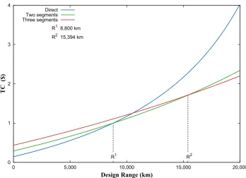
We illustrate these cutoff thresholds graphically.
Using the same numerical estimates as in previous sections15 we plot (in Figure 4) the FPR
against design range for a direct flight, an itinerary segmented into two equal halves, and an
itinerary segmented into three equal thirds. Recall that Figures 1 and 2 both suggest that the
highest efficiency for a single-hop flight (a single takeoff-landing pair) is achieved at a design
range of 3,872km. For distances shorter than 5,433km, dividing the itinerary would result in
segments much shorter than the optimal 3,872km and thus a lower efficiency for the itinerary
overall. Therefore the direct flight remains the most fuel- and hence GHG-efficient. For distances
between 5,433km and 9,462km, an itinerary segmented into two equal halves is most efficient,
as the fuel burn of a direct flight is considerably higher due to the inefficiently high fuel-load
burden it requires. For distances above 9,462km, an itinerary segmented into three equal thirds
becomes most efficient.
Exploiting the TVI interpretation of the FPR curve, we can re-examine the flight-segmentation
problem from the standpoint of minimizing Total Cost (TC). Using the same price for jet
fuel as was used above in Figure 3 (0.6548 $/kg) and maintaining the assumption that Fixed
Cost (FC) per payload kg per leg is 10¢, we plot (in Figure 5) the TC against design range
for a direct flight, an itinerary segmented into two equal halves, and an itinerary segmented
into three equal thirds. Notice that there are large differences between the technically
effi-cient segmentation thresholds (5433km and 9462km) and the economically effieffi-cient
flight-segmentation thresholds (8800km and 15394km) – even when FC is limited to a very modest
10¢ per payload kg per leg.
15
Figure 4: Fuel-Payload Ratio against design range: direct flight, two-segment itinerary, and three-segment itinerary.
0 0.5 1 1.5 2 2.5
0 5,000 10,000 15,000
R1 5,433 km R2 9,462 km
FPR (kg/kg)
Design Range (km) Direct
Two segments Three segments
R1
R1 RR22
Figure 5: Total Cost against design range: direct flight, two-segment itinerary, and three-segment itinerary; Fixed Cost component of TC is 10¢ per payload kg per leg.
0 1 2 3 4
0 5,000 10,000 15,000 20,000
R1 8,800 km R2 15,394 km
TC
($)
Design Range (km) Direct
Two segments Three segments
R1
[image:16.595.123.472.425.677.2]4 Sensitivity analysis
Green (2002) analyzes the sensitivity of optimal design range to pertubations in the parameters
c1andc2, concluding thatc2does not affect the optimal design range while the effect ofc1can be
approximated with a quadratic function. In this study we focus on two other key parameters:
λ (the lost-fuel fraction of aircraft weight at takeoff) and X (the aircraft range parameter).
Hence the present study is distinct from, but complements that undertaken in Green (2002).
We examine the effects of pertubations in λ and X on optimal design range as well as on the
cutoff thresholds that demarcate between optimal one-leg, two-leg, and three-leg segmentation,
for both fuel-saving (and hence GHG-saving) and Total-Cost-saving considerations.
Table 2 shows the impact of varying the lost-fuel fractionλ. We continue to use 2.2% as the
base value for λ, and we present six scenarios of +/− 5%, +/− 10% and +/−20%. For each
scenario, the optimal design range and optimal segmentation thresholds are recorded in columns
2–7, together with the associated percentage changes in parentheses. Several conclusions can be
drawn from Table 2.
First, an increase in the lost-fuel fractionλat takeoff leads to longer optimal design range. As
more fuel is consumed during takeoff, climb-to-cruise altitude and acceleration-to-cruise speed,
the efficiency of short-distance flights drops more sharply than that of longer-distance flights as
any increase in λ has a smaller effect due to (averaging over) the higher total mission fuel of
longer-distance flights.
Second, as λ increases, the increase in optimal design range leads to higher optimal cutoff
thresholds between single-leg and two-leg flights, as well as between two-leg and three-leg flights.
When optimal design range is displaced to the right – e.g. as the result of an increase in λ –
splitting a journey into separate legs becomes advantageous only at even longer ranges where
FPR convexity accelerates the inefficiency penalty accruing from incremental increases in flight
distance.
Third, all three variables (columns 2–7) have a closely fitting log-log-linear relationship with
λ.16 For fuel-saving consideration, a 1% change in λ leads to a 0.425% change in optimal
design range, a 0.421% change in the two-segment threshold, and a 0.423% change in the
three-16
segment threshold. When minimizing TC instead, a 1% change inλ leads to a 0.100% change
in optimal design range, a 0.098% change in the two-segment threshold, and a 0.100% change
in the three-segment threshold. Switching from fuel-saving to TC-saving attenuates sensitivity
[image:18.595.73.524.198.318.2]to pertubations inλ. Note that these changes are of the same algebraic sign as the change inλ.
Table 2: Sensitivity of optimal design range and cutoff thresholds to changes in the lost-fuel fractionλ.
Lost-fuel Optimal Two-segment Three-segment Optimal Two-segment Three-segment fraction (λ) design range threshold threshold design range threshold threshold
(fuel-saving) (fuel-saving) (fuel-saving) (TC-saving) (TC-saving) (TC-saving)
1.76% (-20%) 3,520 (-9.09%) 4,947 (-8.95%) 8,612 (-8.98%) 6,188 (-2.01%) 8,626 (-1.98%) 15,084 (-2.01%) 1.98% (-10%) 3,702 (-4.39%) 5,196 (-4.36%) 9,047 (-4.39%) 6,253 (-0.98%) 8,712 (-1.00%) 15,235 (-1.03%) 2.09% (-5%) 3,789 (-2.14%) 5,320 (-2.08%) 9,264 (-2.09%) 6,285 (-0.48%) 8,757 (-0.49%) 15,317 (-0.50%) 2.2% (0%) 3,872 (0%) 5,433 (0%) 9,462 (0%) 6,315 (0%) 8,800 (0%) 15,394 (0%) 2.31% (+5%) 3,953 (+2.09%) 5,543 (+2.02%) 9,655 (2.04%) 6,348 (+0.52%) 8,844 (+0.50%) 15,470 (+0.49%) 2.42% (+10%) 4,031 (+4.11%) 5,655 (+4.09%) 9,852 (4.12%) 6,379 (+1.01%) 8,884 (+0.95%) 15,543 (+0.97%) 2.64% (+20%) 4,179 (+7.93%) 5,880 (+8.23%) 10,246 (8.29%) 6,439 (+1.96%) 8,973 (+1.97%) 15,695 (+1.96%)
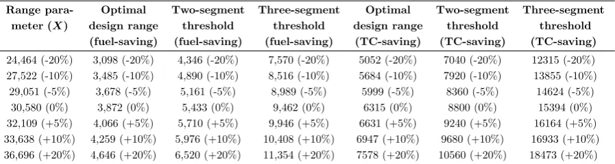
Table 3 reports the corresponding responses to pertubations of the aircraft range parameter
X. Clearly the optimal design range for single-hop flights as well as the segmentation thresholds
are proportional to X. This is because X enters the FPR (11) equations – and therefore also
the segmentation thresholds (15) and (16) – as the denominator to R. Therefore when holding
optimal rangeR∗ and all other parameters constant, an arbitraryd% (d%6= 0%) pertubation of
X renders the originalR∗ suboptimal. The first-order condition is restored, however, by scaling
R∗ by the same d% pertubation. The level of the optimal FPR is left unchanged, although
the optimal design range at which this occurs is scaled by d% (see column 2). Inspection of
equations (15) and (16) confirms that this is true also for the optimal segmentation thresholds
[image:18.595.74.523.611.731.2](see columns 3–7).
Table 3: Sensitivity of optimal design range and cutoff thresholds to changes in the aircraft range parameter X.
Range para- Optimal Two-segment Three-segment Optimal Two-segment Three-segment
meter (X) design range threshold threshold design range threshold threshold
(fuel-saving) (fuel-saving) (fuel-saving) (TC-saving) (TC-saving) (TC-saving)
24,464 (-20%) 3,098 (-20%) 4,346 (-20%) 7,570 (-20%) 5052 (-20%) 7040 (-20%) 12315 (-20%)
27,522 (-10%) 3,485 (-10%) 4,890 (-10%) 8,516 (-10%) 5684 (-10%) 7920 (-10%) 13855 (-10%)
29,051 (-5%) 3,678 (-5%) 5,161 (-5%) 8,989 (-5%) 5999 (-5%) 8360 (-5%) 14624 (-5%)
30,580 (0%) 3,872 (0%) 5,433 (0%) 9,462 (0%) 6315 (0%) 8800 (0%) 15394 (0%)
32,109 (+5%) 4,066 (+5%) 5,710 (+5%) 9,946 (+5%) 6631 (+5%) 9240 (+5%) 16164 (+5%)
33,638 (+10%) 4,259 (+10%) 5,976 (+10%) 10,408 (+10%) 6947 (+10%) 9680 (+10%) 16933 (+10%)
5 Conclusion
In this study we develop a fuel-efficiency model for scheduled passenger air transport built on
K¨uchemann’s (1978) Weight Model and the Breguet Range Equation for cruise fuel consumption.
Through a numerical example we show how the model sheds light on the effect of aircraft
design range on fuel efficiency. Importantly, it is possible to determine fuel-efficiency-maximizing
optimal design range.
Then we introduce a new efficiency metric, the Fuel-Payload Ratio, as an alternative to
complement the existing Payload Fuel Efficiency metric. We show that this new metric verifies
the conventional representation of the model and furthermore complements the model with new
findings. While the PFE curve perfectly captures changing fuel efficiency as a single aircraft
is designed for a longer range, FPR gives guidance on how to compare the efficiency levels of
multiple aircraft with different design ranges, when aircraft can be grouped to serve a flight
route that contains multiple segments. Using the same set of model parameters, we find the
cut-off thresholds demarcating between efficiency of a direct flight, an itinerary with two equal
segments, and an itinerary with three equal segments.
Moreover, the direct interpretation of FPR as the lower envelope of Total Variable Input
curves allows the technical engineering analysis exemplified in Green (2002) to be integrated
with the standard cost-curves-based microeconomic efficiency analysis. In this framework we
have shown that additional fixed costs on payload have the effect of increasing the cost-efficient
design range, causing the latter to diverge from the technically efficient design range. Hence
factors that increase payload fixed costs – regardless of where these costs originate from – can
have the unintended consequence of contributing to ‘wrong sizing’ of the aircraft stock from the
standpoint of fuel efficiency and GHG emissions. Those same factors entail that economically
efficient flight-segmentation thresholds occur at much greater origin-destination distances than
those which would minimize fuel consumption and GHG emissions.
We study the sensitivity of optimal design range and the cut-off distances for different
itinerary structures to model parameters. As the lost fuel fraction λ increases, all the three
ranges increase. A 1% change in λwill lead to a 0.421%–0.425% change in the thresholds
un-der pure fuel-saving optimization, and a 0.098%–0.100% change in the thresholds unun-der pure
lead to proportionate changes in the thresholds.
References
Campbell, S.E, Bragg, M.B., Neogi, N.A., 2013. Fuel-optimal trajectory generation for persistent
contrail mitigation. Journal of Guidance, Control, and Dynamics 36 (6), 1741–1750.
Cansino, J.M, Rom´an, R., 2017. Energy efficiency improvements in air traffic: The case of Airbus
A320 in Spain. Energy Policy 101, 109–122.
Chi, J., Baek, J., 2012. Price and income elasticities of demand for air transportation: Empirical
evidence from US airfreight industry. Journal of Air Transport Management 20, 18–19.
Dallara, E.S., 2011. Aircraft Design for Reduced Climate Impact. PhD Dissertation, Stanford
University, Stanford, CA.
Dallara, E.S., Kroo, I.M., 2011. Aircraft design for reduced climate impact. 49thAIAA Aerospace
Sciences Meeting, 4–7 January 2011, Orlando, FL.
Dalmau, R, Prats, X., 2015. Fuel and time savings by flying continuous cruise climbs: Estimating
the benefit pools for maximum range operations. Transportation Research Part D 35, 62–71.
Dumas, J., Aithnard, F., Soumis, F., 2009. Improving the objective function of the fleet
assign-ment problem. Transportation Research Part B 43 (4), 466–475.
Fielding, J.P., 1999. Introduction to Aircraft Design. Cambridge University Press, Cambridge,
England.
Gallet, C.A., Doucouliagos, H., 2014. The income elasticity of air travel: A meta-analysis. Annals
of Tourism Research 49, 141–155.
Green, J.E., 2002. Greener by design – the technology challenge. Aeronautical Journal 106
(1056), 57–113.
Green, J.E., 2006. K¨uchemann’s weight model as applied in the first greener by design technology
sub group report: A correction, adaptation and commentary. Aeronautical Journal 109 (1099),
Green, J.E., 2009. The potential for reducing the impact of aviation on climate. Technology
Analysis and Strategic Management 21 (1), 39–59.
IATA, 2008. Air Travel Demand. International Air Transport Association (IATA) Economics
Briefing No. 9, Geneva, Switzerland.
ICAO, 2012. ICAO Carbon Emissions Calculator, version 5. International Civil Aviation
Orga-nization (ICAO), Montr´eal, Canada. https://www.icao.int/environmental-protection/
CarbonOffset/Documents/Methodology%20ICAO%20Carbon%20Calculator_v5-2012.
Revised.pdf
Kaivanto, K., Zhang, P., 2017. Rank-order concordance among conflicting emissions estimates
for informing flight choice. Transporation REsearch Part D 50, 418–430.
K¨uchemann, D., 1978. The Aerodynamic Design of Aircraft. Pergamon Press, Oxford.
Langhans, S., Linke, F., Nolte, P., Gollnick, V., 2013. System analysis for an intermediate stop
operations concept on long range routes. Journal of Aircraft 50 (1), 29–37.
Lee, J.J., Lukachko, S.P., Waitz, I.A., Schafer, A., 2001. Historical and future trends in aircraft
performance, cost and emissions. Annual Review of Energy and the Environment 26, 167–200.
Li, Z.-C., Lam, W.H.K., Wong, S.C., Fu, X., 2010. Optimal route allocation in a liberalizing
airline market. Transportation Research Part B 44, 886–902.
Martinez-Val, R., Perez, E., Cuerno, C., Palacin, J.F., 2013. Cost-range trade-off of intermediate
stop operations of long-range transport airplanes. Proceedings of the Institution of Mechanical
Engineers Part G: Journal of Aerospace Engineering 227 (2), 394–404.
Nangia, R.K., 2006. Efficiency parameters for modern commercial aircraft, Aeronautical Journal
110 (1110), 495–510.
Perez, R.E., Jansen, P.W., 2014. Design optimization and staging assignment for long-range
aircraft operations. In AVIATION 2014, AIAA/3AF Aircraft Noise and Emissions Reduction
Symposium, 16–20 June 2014, Atlanta Georgia.
Pita, J.P., Adler, N., Antunes, A.P., 2014. Socially-oriented flight scheduling and fleet assignment
Poll, D.I.A., 2011. On the effect of stage length on the efficiency of air transport. Aeronautical
Journal 115 (1167), 273–283.
Torenbeek, E., 1997. Cruise performance and range prediction reconsidered, Progress in
Aerospace Sciences 33 (5/6), 285–321.
Yutko, B.M., Hansman, R.J., 2011. Approaches to representing aircraft fuel efficiency
perfor-mance for the purpose of a commercial aircraft certification standard. MIT International
Center for Air Transportation, Department of Aeronautics & Astronautics, MIT, Cambridge,
MA.
Zeinali, M., Rutherford, D., 2010. Trends in aircraft efficiency and design parameters.
Interna-tional Council on Clean Transportation, Washington, DC. http://www.theicct.org/2010/
A Mathematical appendix
Noting that the first three derivatives of the FPR function are positive,
FPR =f(R) where f0, f00, f000 >0 ∀R∈R++ (17)
denote the midpoint of the Great-Circle Distance between the origin and the destination airports
Rkm apart as R0 =R/2. Let us conjecture that the minimum whole-itinerary FPR is achieved in a two-leg segmentation when both legs are of length R0. With this segmentation, the total FPR is 2f(R0). Shortening one leg by 4 ∈(0,0.5] entails increasing the length of the other leg by the same amount 4 so that total itinerary length remains 2R0. Now total itinerary FPR may be written as f(R0− 4) +f(R0+4). From f000 >0 it follows that
|f(R0− 4)−f(R0)|< f(R0+4)−f(R0) (18)
and therefore that
f(R0− 4) +f(R0+4)>2f(R0) ∀ 4 ∈(0,0.5] (19)
i.e. that total itinerary FPR is greater under any other division of the total distance than the
equal-length-legs segmentation.
Similar reasoning applies in the three-leg case. RedefiningR0 asR0=R/3, let us conjecture that the minimum whole-itinerary FPR in the three-leg segmentation is 3f(R0). Define three signed deviation terms 41,42,43 ∈ [−0.5,0.5] representing the deviation of legs 1, 2 and 3 from R0 respectively. These deviation terms satisfy 41+42+43 = 0, giving (R0 +41) + (R0+42) + (R0+43) = 3R0.
If 41,42<0 then 43=|41|+|42|; if 41,43 <0 then 42=|41|+|43|; if 42,43 <0 then 41 =|42|+|43|. From f000 >0 it follows that when 41,42 <0,
|f(R0+41)−f(R0)|+|f(R0+42)−f(R0)|< f(R0+|41|+|42|)−f(R0) (20)
and similarly when 41,43<0 and when 42,43 <0.
If 41,42 > 0 then 43 = −(41 +42); if 41,43 > 0 then 42 = −(41 +43); if 42,43 >0 then 41 =−(42+43). From f000>0 it follows that when 41,42 >0,
and similarly when 41,43>0 and when 42,43 >0.
If ∃ 4i= 0, i∈ {1,2,3}, then either there is only one such zero deviation and the problem reduces to that depicted in equations (18) and (19), or then all deviations are zero 4i= 0, ∀i∈ {1,2,3}.
Therefore
f(R0+41) +f(R0+42) +f(R0+43)≥3f(R0) ∀ 4i∈[−0.5,0.5], 3 X
i=1
4i = 0 (22)
i.e. total itinerary FPR is greater under any other division of the total distance than the three
Highlights
• We derive the Fuel-Payload Ratio (FPR) for parsimoniously segmenting itineraries
• Microeconomic analogue of FPR is Total Variable Input curve with respect to design range
• Economically and technically efficient design ranges diverge due to fixed costs on payload
• Fuel-saving segmentation thresholds respond ≥0.42 :1 to lost-fuel fraction (λ) %-increases
A Supplementary Appendix: Responses to Reviewers’ comments
The authors wish to express their gratitude to the Editor and the Reviewers for these first-round
comments, which we find to be valuable and constructive.
In what follows, Reviewers’ text is coded red. Text cited from the original (first) review draft
is codedblue. Authors’ discussion of Reviewers’ comments is codedblack. Text altered in the body of the article is codedmagenta.
Reviewer 1
R1.1 “Authors should make a greater effort explaining why this issue is important. The first
paragraph starts with the methods for calculating GHG but the problem has not been
contextualized.”
Response: We fully concur with the Reviewer.
Remedy: We have introduced two new lead-in paragraphs, the purpose of which is to
provide appropriate contextualization.
New text, p 2: Air transportation is caught between two converging forcing
boundaries. The first is increasing demand for air transportation, driven by
income growth – notably, at a rate faster than income growth itself – during an
era of consistently increasing world Gross Domestic Product (GDP).
[foot-note: In the post-1970s era, GDP has consistently grown, with the exception
of one year in which the world economy absorbed the fallout from the financial
crisis (2009). The empirical income elasticity of demand for air transportation
services is widely documented to be greater than 1: for every 1% increase
in income (i.e. GDP), demand for air transport increases by more than 1%
(IATA, 2008; Chi and Baek, 2012; Gallet and Doucouliagos, 2014).] The
sec-ond is accelerating anthropogenic climate change, and the consequent need to
reduce greenhouse gas (GHG) emissions drastically in order to avoid
global-ecosystem-altering climate change. Technological innovation and far-reaching
policy changes will be required in the medium term in order to achieve the
targets agreed to in the United Nations Framework Convention on Climate
In the short run, the greenhouse gas (GHG) footprint of air transportation
can be reduced by optimizing aircraft design-and-deployment decisions within
the envelope of current technological possibility.
R1.2 “In the introduction section, some acronyms have to be defined the first time is used in
the manuscript, i.e. ICAO.”
Response: We thank the Reviewer for detecting these omissions.
Remedy: We have now ensured that all acronyms and initialisms are defined.
R1.3 “Sections 2, and 3 explain the methodologies that authors have followed in each part of
the analysis but they should be linked further previously in the introduction section in
order to help readers to understand the complete analysis.”
Remedy: We revise the introduction to provide the reader with a roadmap of how Section
2 lays the theoretical groundwork upon which Section 3 builds to derive the FPR metric
and the flight-segmentation results.
Revised text, p 3: In Section 2 we investigate the impact of design range on
commercial air transport fuel efficiency by developing a model drawing on
K¨uchemann’s (1978) Weight Model and the Breguet Range Equation for cruise
fuel consumption. ... ...We build on this in Section 3 to introduce a new
efficiency metric, the Fuel-Payload Ratio (FPR), which captures the
techni-cal relationship between mission fuel burn and payload transported to design
range. With the aid of this FPR metric, identification of optimal design range
(Section 3.2), as well as optimal thresholds for 1-, 2-, and 3-segment flights
(Section 3.3), is straightforward. Furthermore, 1/FPR may be understood
as a short-run production function in a standard microeconomic sense, from
which it follows that the standard short-run curves – marginal and average
product, variable cost and total cost, marginal cost, average variable cost and
average total cost – may also be derived straightforwardly. This makes it
pos-sible to undertake economic optimization of the design-range decision
parsimo-niously, without abstracting from any of the engineering information contained
in Green’s (2002) PFE metric. We conclude with a sensitivity analysis (Section
in Green (2002).
R1.4 “I would suggest to explain further [in] the literature review at the beginning explaining
the reason why these three methodologies are applied. Which are the connexions among
them?”
Remedy: We follow the Reviewer’s suggestion. The introduction now includes new text
that primes the reader to the methodological choices made, and to the connections between
the elements of the subsequent analysis.
New text, p 4: ...These two equation families complement each other. K¨uchemann’s
(1978) Weight Model is a standard if not classic [footnote: Dietrich K¨uchemann
is thought by some to be the finest aerodynamicist of his generation. His
posthumously published (1978)The Aerodynamic Design of Aircraft is widely
regarded as a classic text in aerodynamics.] decomposition of aircraft
take-off weight into components that roughly correspond to airframe empty weight,
payload, engines, and mission fuel. The Breguet Range Equation in turn
al-lows cruise range to be expressed as a function of (i) aircraft initial weight at
take-off, (ii) aircraft ‘final weight’ upon landing, after mission fuel has been
consumed, and (iii) range-performance parameters capturing the calorific
en-ergy content of the fuel, the propulsive efficiency of the engine, and the aircraft
design’s lift-to-drag ratio. By substituting terms from one equation into the
other and accounting for fuel consumed in propelling the aircraft from the
blocks all the way to cruise speed and altitude, Green (2002) derived the
Pay-load Fuel Efficiency (PFE) metric, defined as the product of range and the ratio
of the weight of payload to mission fuel. We build on this in Section 3 to
intro-duce a new efficiency metric, the Fuel-Payload Ratio (FPR), which captures
the technical relationship between mission fuel burn and payload transported
to design range. With the aid of this FPR metric, identification of optimal
de-sign range (Section 3.2), as well as optimal thresholds for 1-, 2-, and 3-segment
flights (Section 3.3), is straightforward. ...
R1.5 “In section 4, sensitivity analysis, there is no reference or comparison of the results with
implemented.”
Response: Whereas Green’s (2002) sensitivity analysis investigates the effects of
pertuba-tions of parametersc1 and c2, the sensitivity analysis conducted in Section 4 of this paper
investigates the effects of pertubations of λ(the ‘lost-fuel’ fraction of take-off weight) and
X (the aircraft range parameter). Hence the Section 4 sensitivity analysis complements
rather than competes with Green’s (2002) sensitivity analysis. A like-for-like comparison
with other sensitivity analyses is not possible for this reason.
Remedy: We clarify the complementary nature of the sensitivity analyses conducted in
this paper and in Green (2002) in the introduction as well as at the beginning of Section
4.
Revised text, p 4: We conclude with a sensitivity analysis (Section 4) that
com-plements rather than replicates the sensitivity analysis undertaken in Green
(2002).
Revised text, p 17: Green (2002) analyzes the sensitivity of optimal design range
to pertubations in the parametersc1 andc2, concluding that c2 does not affect
the optimal design range while the effect of c1 can be approximated with with
a quadratic function. In this study we focus on two other key parameters: λ
(the lost-fuel fraction of aircraft weight at takeoff ) and X (the aircraft range
parameter). Hence the present study is distinct from, but complements that
undertaken in Green (2002).
R1.6 “More efforts should be done by authors to be understood by no specialized readers.”
Response: In addressing the Reviewer’s comments R1.1-5 – as well as in addressing
Re-viewer #2’s comments R2.1-4 – we have aimed for clarity and simplicity. For instance, we
have cut some of the detail on the FPR in the abstract. We have also introduced guidance
for the non-specialist in the introduction (see new text above associated with R1.1). In
the main body of the text, where simplification would entail glossing over relevant
dis-tinctions, we employ structure to aid the reader. For instance as detailed in R1.3, we
explain the Breguet Range Equation as consisting of components (i), (ii), (iii). Also, we
have added further summary and explnation of our results, such as the following addition
New text, p 19: Moreover, the direct interpretation of FPR as the lower
enve-lope of Total Variable Input curves allows the technical engineering analysis
exemplified in Green (2002) to be integrated with the standard
cost-curves-based microeconomic efficiency analysis. In this framework we have shown
that additional fixed costs on payload have the effect of increasing the
cost-efficient design range, causing the latter to diverge from the technically cost-efficient
design range. Hence factors that increase payload fixed costs – regardless of
where these costs originate from – can have the unintended consequence of
contributing to ‘wrong sizing’ of the aircraft stock from the standpoint of fuel
efficiency and GHG emissions. Those same factors entail that economically
ef-ficient flight-segmentation thresholds occur at much greater origin-destination
distances than those which would minimize fuel consumption and GHG
emis-sions.
Reviewer 2
R2.1 “... it is not clear the exact contribution with respect to what was already proposed by
Green in his previous publications. The new proposed metric is quite similar to already
existing metrics and does not seem to provide more insights into the problem assessed. I
would like to see a more clear justification of the novelty and contribution of the research
done.”
Response: Reflecting upon the Reviewer’s comment, we have come to agree that it is
nec-essary to articulate more clearly this paper’s novel contribution and the way in which it is
distinguished from & goes beyond the preceding substantive work by Green (2002, 2006).
As it happens, the work program reported here was designed from its very inception to
complement Green’s (2002) analysis. Any one study – including Green’s (2002)
57-page-long, broad-ranging paper – must be somehow limited and bounded in its aspirations.
Briefly, our paper’s novelty and distinctness occurs in three dimensions.
First, the Fuel-Payload Ratio (FPR) efficiency measure – although derived from the same
set of equations Green (2002, 2006) employs – has a direct interpretation in the standard
microeconomic framework as the lower envelope of Total Variable Input (TVI) curves,
6 for illustration).
We now appreciate that this statement in itself is not equally meaningful to all readers, and
hence requires elaboration. Responding to this need for elaboration, we introduce an
illus-tration of how Fixed Costs affect Average-Total-Cost-minimizing design range (detailed
below in Remedy #2), thereby contributing to our understanding of the empirical
dispar-ity between the design ranges of aircraft purchases (and stock thereby created) based on
economic drivers and the design ranges of aircraft purchases (and associated stock created)
if they were guided purely by technical (fuel, GHG) efficiency.
Second, the present study of flight segmentation aims to sharpen Green’s (2002) somewhat
vague suggestions concerning stage length, i.e.
...it seems likely that a large aircraft designed to cover long distances in stages
of typically, say, 5,000km would have significantly lower seat kilometre costs...
(Green 2002, p 61)
...We recommend that a full study be undertaken of the engineering, operational,
infrastructure, safety, market, economic and total environmental implications of
providing long distance air travel in multi-sector journeys, with no sector longer
than, say, 7,500km. (Green 2002, p 61)
...In the full report ... leads to the suggestion that the most environmentally
friendly solution might be to break long journeys into sectors not exceeding
7,500km... (Green 2002, footnote, p 61)
Hence the present study is distinct from, but responds to, complements, and sharpens
Green (2002).
The advantage of the FPR-based approach is that its mathematical form provides
straight-forward answers to these types of questions.
Third, the sensitivity analysis reported in this study investigates the effects of
varia-tions/pertubations in λ and X – whereas Green’s (2002) sensitivity analysis studies the
effects of varying c1 and c2. Hence the present study is distinct from, but complements
Green (2002).
Remedy #1: In order to ensure that the paper’s findings are more clearly identified and
New headings, pp. 8–11:
Finding 3.1 Mission fuel increases with R, at an accelerating rate
Finding 3.2 min FPR/km design range = R∗
Finding 3.3 FPR-based mission fuel is validated by ICAO data
Finding 3.4 Standard microeconomic interpretation
Remedy #2: To illustrate the distinctness of FPR-based analysis and the significance of
the standard microeconomic analysis tools that this formulation avails, we illustrate the
effect tht a 10¢ increase in Fixed Cost has on economically efficient design range.
New text, pp. 11: Placing FPR within a microeconomic framework leads to
insights that are typically not available within a purely technical engineering
analysis. For instance, FPRR =
WMF
WP
may be re-expressed in
monetary-unit terms by multiplying equation (11) by the price of kerosene ($/kg) – i.e.
the vertical axis of Figure 2 may be re-indexed by multiplying by the price of
kerosene, which at the time of writing is 654.8 $/mt or 0.6548 $/kg (see Figure
3).17 On this cost scale, the FPR becomes the lower envelope of Total Variable
Cost (TVC) curves. This opens up the possibility of investigating the effect
of changes in Fixed Costs (FC) on cost-efficient choice of design range –
re-gardless of whether those Fixed Costs arise from engineering, regulatory (e.g.
environmental regulations), safety and service, or other business-environment
considerations. Figure 3 illustrates how a 10¢ increase in Fixed Cost18
in-creases Average-Total-Cost-minimizing design range by over 2,400 km.
This microeconomic analysis of the effect of Fixed Costs carries two types of
implications. First, it goes some way to explaining why the stock of aircraft
operated on short- and medium-length segments are ‘oversized’ in terms of
design range: economic considerations rather than purely technical fuel- and
GHG-effiiciency considerations weigh heavily in the aircraft purchase decision.
Second, it shows the unintended consequences of introducing regulations –
whether motivated by environmental-protection concerns or not – that increase
payload Fixed Cost.
17
Jet fuel price obtained from the IATA Jet Fuel Price Monitor on 30 March 2018. http://www.
iata.org/publications/economics/fuel-monitor/Pages/index.aspx
18
Figure 3: Total Variable Cost (TVC) and Total Cost (TC) envelopes against design range, where Fixed Cost (FC) is 10¢ per payload kg.
0 1 2 3 4
0 5,000 10,000 15,000 20,000
R* 6,315 km
TVC,TC
($)
Design Range (km)
TVC(R) TC(R)=FC+TVC(R)
R* R*
Remedy #3: In order to highlight the novelty and precision of the FPR-based approach to
determining optimal flight segmentation, we reformat Section 3.3’s introductory-paragraph
structure as follows. The mathematical structure presented through equations (15) and
(16), and associated proof in Appendix A, are self explanatory.
Reformatted text, p 13 : Answers to these questions are not straightforward from
the PFE-based analysis.
The Fuel-Payload Ratio curve, on the other hand, provides straightforward
answers to these questions.
Since FPR represents the ideal mission-fuel consumption to deliver a one-unit
payload to a specified range, when the same unit payload is delivered through
segments, the sum of segment-specific FPR ratios represents the total mission
fuel for the whole itinerary, assuming that the ideal aircraft (with appropriate
design range) is used on each segment. As the FPR curve is convex in design
range, this offers unambiguous guidance for minimizing the sum.
Remedy #4: We revise Section 4’s introductory paragraph to emphasize that the present
Original text, p 13: Green (2002) discusses the sensitivity of optimal design range
to the parameters c1 and c2, concluding that c2 does not affect the optimal
de-sign range while the effect ofc1 can be approximated with a quadratic function.
In this study we focus on two other key parameters: λ (the lost-fuel fraction
of aircraft weight at takeoff ) and X (the aircraft range parameter).
Revised text, p 17: Green (2002) analyzes the sensitivity of optimal design range
to pertubations in the parametersc1 andc2, concluding that c2 does not affect
the optimal design range while the effect of c1 can be approximated with with
a quadratic function. In this study we focus on two other key parameters: λ
(the lost-fuel fraction of aircraft weight at takeoff ) and X (the aircraft range
parameter). Hence the present study is distinct from, but complements that
undertaken in Green (2002).
Remedy #5: In the conclusion we include an additional paragraph that summarises some
of the further implications of the FPR-based approach.
Revised text, p 19: Moreover, the direct interpretation of FPR as the lower
en-velope of Total Variable Input curves allows the technical engineering analysis
exemplified in Green (2002) to be integrated with the standard
cost-curves-based microeconomic efficiency analysis. In this framework we have shown
that additional fixed costs on payload have the effect of increasing the
cost-efficient design range, causing the latter to diverge from the technically cost-efficient
design range. Hence factors that increase payload fixed costs – regardless of
where these costs originate from – can have the unintended consequence of
contributing to ‘wrong sizing’ of the aircraft stock from the standpoint of fuel
efficiency and GHG emissions. Those same factors entail that economically
ef-ficient flight-segmentation thresholds occur at much greater origin-destination
distances than those which would minimize fuel consumption and GHG
emis-sions.
R2.2 “The values given for c1 and c2 coefficients seem very arbitrary. Moreover, are they the
same for all type of aircraft?”
conveys the impression that the coefficients are somewhat arbitrarily ‘set’. The sourcing
of the values for c1 and c2 is detailed at the beginning of Section 2.3. Nevertheless, we
very much agree with the Reviewer that this passage requires re-phrasing and elaboration.
The parameters capture the way in which fuel (GHG) efficiency changesacross aircraft of
different design range, and areestimated from data on 12 different wide-body swept-wing
kerosene-fuelled aircraft.
Remedy: We rewrite the paragraph in which the coefficient values are introduced, with the
intent of clarifying that these are in actual fact estimated values, rather than values that
are arbitrarily ‘set’. And in a footnote, we introduce more detail on how the coefficients
have been estimated.
These parameter values are also mentioned at the beginning of Section 3.2 on p 8, as well
as in Section 3.3 on p 11. In each case, we rewrite the text, paying careful attention to
word choice, and we refer the reader back to Section 3.2 for details.
Original text, p 6: In order to illustrate how PFE varies with design range,
pa-rameter values need to be set for X, c1 and c2. Fielding (1999) introduces a
method for estimating the values of c1 and c2. Green (2002) adopts 0.3 for c1
and 2.0 for c2 for swept-wing kerosene-fuelled aircraft. Green (2006) points
out that when reserve fuel is present, c1 must be adjusted upwards. Following
Nangia’s (2006) proposed value of 4.5% of total weight at takeoff as reserve
fuel, Green (2006) adjusting c1 to 0.345. To maintain comparability, we also
follow Green (2002) in setting the aircraft range parameterX to be 30,580km
and the lost-fuel fraction λto be 2.2%.
Revised text, page 7: In order to illustrate how PFE varies with design range,
parameter values need to be determined for X, λ, c1 and c2. Using Fielding’s
(1999) data, Green (2002, 2006) estimates c2 to be 2.0. Green (2006) revisits
the estimation ofc1 in light of Nangia (2006), and using Fielding’s (1999) data
Green (2006) estimates c1 to be 0.345. [footnote: These values for c1 and
c2 are obtained by fitting OEW = (c1 −0.045)WTO + (c2 −1)WP to Fielding’s
(1999) Table A4.5 (page 188) data on twelve modern wide-body, swept-wing,
kerosene-fueled passenger aircraft, where the parameter0.045reflects Nangia’s
(Green, 2006).] We also follow Green (2002, 2006) in employing the aircraft
range parameter X = 30,580km and the lost-fuel fraction λ= 2.2%.
Original text, p 8: In this numerical example, we continue to follow Green (2002)
in setting 2.0 for c2 for a swept-wing kerosene-fueled aircraft, and we follow
Green (2006) and Nangia (2006) in correcting c1 upwards from 0.3 to 0.345.
Again we follow Green (2002) in setting the aircraft range parameter X to
30,580km and the lost-fuel fraction λ to 2.2%.
Revised text, page 9: In this numerical example, we continue to employ the
pa-rameter values introduced above in Section 2.3. [footnote: c1 = 0.345, c2 = 2.0,
λ= 2.2%, X = 30,580km]
Original text, p 11: Using the same numerical assumptions as in previous
sec-tions, [footnote: We set 2.0 for c2 for a swept-wing kerosene-fueled aircraft,
and follow Green (2006) and Nangia (2006) in correcting c1 upwards to 0.345.
Again we follow Green (2002) in setting the aircraft range parameter X to
30,580km and λ to 2.2%.] we plot ...
Revised text, page 14: Using the same numerical estimates as in previous
sec-tions [footnote: c1 = 0.345, c2 = 2.0, λ= 2.2%, X= 30,580km] we plot ...
R2.3 “Details on the ICAO data used to assess the FPR curve in figure 2 are missing. At least
give a bibliographic reference.”
Response: We thank the Reviewer for spotting this omission.
Remedy: Full reference is provided in a footnote.
Revised text, page 10: Table 1 contains ICAO data on flight range, average
mission-fuel consumption and average number of seats (columns 3–5). [footnote:
ICAO (2012) documents the methodology by which the average fuel (kg) data
have been compiled. The approach employed draws primarily from the EMEP/
CORINAIR Emission Inventory Guidebook, following IPCC guidance.]
R2.4 “As a minor suggestion, the authors may consider the following (or similar) two
publica-tions to cite in their introduction. These tackle the problem of the flight plan optimisation,
Response: These are helpful suggestions, and have been integrated into the revisions
requested by Reviewer 1 to make the paper more accessible to non-specialized readers,