Clustering Algorithms for Huge Datasets: A Mathematical Approach

Clustering Algorithms for Huge Datasets: A

Mathematical Approach

Shyam Mohan J. S.

Assistant Professor, Dept. Of CSE, SCSVMV, Enathur, Kanchipuram, Tamilnadu, India

Shanmugapriya P.

Associate Professor, Dept. Of CSE, SCSVMV, Enathur, Kanchipuram, Tamilnadu, India

ABSTRACT

Identifying clusters for huge datasets are useful for finding out attributes of a particular dataset and thereby providing insights for making effective decision making. In our previous work, we have proved the concept of clustering algorithms for huge datasets theoretically by applying small computations on the available datasets. In this paper, we extend the same work by applying Mathematical calculations for the datasets so as to prove the correctness of our previous work carried out. Our proposed method is applied to various datasets and proved K-Means algorithm mathematically and the experimental calculations performed on various clustering algorithms shows that our approach provides the new idea of clustering techniques that can be applied for any number of huge and complex datasets.

Keywords

Machine Intelligence, Clustering Algorithms

1.

INTRODUCTION

Classifying dataset into groups can be effectively done by Clustering where data points in a particular group share similar features. [1] Some of the applications where Clustering is widely used are: pattern recognition, Customer segmentation, stock market clustering , reduced dimensionality for effective data mining etc.Cluster analysis is done in many ways like K-means, fuzzy means etc.[2][3]

Majority of clustering algorithms fail because of the total number of iterations performed over datasets grows exponentially in size. Big data refers to datasets of huge size. Batch processing or parallel programming technique (MapReduce) provides effective processing of huge datasets. MapReduce is easily scalable that runs on any hardware. The concept of MapReduce is already discussed in our previous works and papers.[4] Parallel programming using MapReduce reduces the time complexity for processing cluster analysis.[5].

2.

BASICS OF DISTANCE AND

SIMILIARITY CALCULATION

For effective clustering, distance (dissimilarity) and similarity measures form the basic idea.[6]. For quantitative datasets, distance is used to find the relationship among data and even similarity features are used for qualitative data.

2.1

Distance Functions

For a normal vector space , the Minkowski distance is used between two points.

Special cases:

 When p=1, It is known as the Manhattan distance.  When p=2, It is known as the Euclidean distance.  In the limit that p --> +infinity, the distance is

known as the Chebyshev distance.

Euclidean distance

For a Euclidean space, distance between two is known as Euclidean distance .

2

Manhattan distance

d(x,y)=

where x and y represent two vectors of length n.

Chebyshev distance

In any vector space, the greatest difference between any coordinate direction is the distance between two vectors.

The correlation distance between two sample vectors in a Pearson's product-momentum is called Pearson correlation distance. The value of correlation coefficient is between [-1, 1], the Pearson distance lies in [0, 2] and measures the linear relationship between the two vectors.

dPearson:(x,y)↦1−Corr(x,y)

Spearman correlation distance

The spearman correlation method is used to compute the correlation between the rank of x and the rank of y variables where x and y sequences are ranked separately. At each position i, the differences in rank are calculated. The distance between sequences X = (X1, X2,……) and Y = (Y1, Y2, ….) is computed using the following formula:

Xi and Yi represent the ith values of X and Y.

In general the value of Spearman Correlation in the range of -1 to -1.

Kendall correlation distance

59

Where P is the set of unordered pairs of distinct elements in

3.

STANDARD K-MEANS

The standard K-means algorithm is an iterative process that guarantees a decrease in total error (value of the objective function f(M)) on each step [7][8].The algorithm is as follows:

1. Choose k initial means s1,s2,---sn , uniformly at random from the set X.

2. For each point xϵX, find the closest mean si and add x to a set Ai.

3. For i = 1,2,----k , set si to be the centroid of the points in Ai.

4. Repeat steps 2 and 3.

5. Step 4 is reached when the optimal solution is obtained. The algorithm takes O(nkd) time for execution.

4.

COMPUTING K-MEANS IN R

Computing K-means in R is done by calculating K-means. This is done by grouping datasets into clusters viz, centers =2, and thereby clusters of 2.We can set the K-means function to start and stop.

Example:

We take two objects A and B with the values tabulated as follows:

Table I : Objects A and B with their coordinate points

values at 1

Values at 2

Values at 3

Values at 4

Values at 5

values at 6

Object A

18 20 30 21 34 32

Object B

100 200 150 300 350 450

Minkowski distance

For input value φ=4,

Minkowski distance = 467.7

Euclidean distance

Object A={18,20,30,21,34,32}

Object B = {100,200,150,300,350,450}

(x,y)={(18,100),(20,200),(30,150),(21,300),(34,350),(32,450)}

Euclidean distance between (18,100) and (32,450) :

d=350.279888

Table II : K-Means Calculation

age spend

Min. :18.00 Min. :100.0

1st Qu.:20.25 1st Qu.:162.5

Median :25.50 Median :250.0

Mean :25.83 Mean :258.3

3rd Qu.:31.50 3rd Qu.:337.5

Max. :34.00 Max. :450.0

Chebyshev distance

Table III : Chebyshev distance Calculation

values at 1

Values at 2

values at 3

values at 4

values at 5

values at 6

Object A

18 20 30 21 34 32

Object B

100 200 150 300 350 450

The Chebyshev distance is 418.

Pearson correlation distance

Table IV : Pearson correlation distance

Values at 1

Values at 2

Values at 3

Values at 4

Values at 5

Values at 6

Object A

18 20 30 21 34 32

Object B

100 200 150 300 350 450

r=0.6241

Spearman correlation distance

R=0.7714

Table V : Kendall correlation distance

Kendall tau Rank Correlation

Kendall tau 0.599999964237213

2-sided p-value 0.13285493850708

Score 9

Var(Score) 28.3333339691162

5.

K-MEANS MAPREDUCE

ALGORITHM (KM-MR)

Input

O :{o1,o2,o3,…..on}; //number of objects to be clustered

X : X number of clusters

Mi : Maximum number of iterations

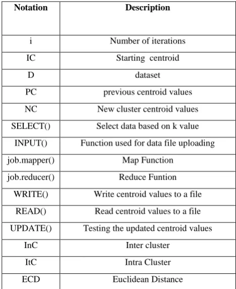
Table VI: Algorithm – Notations used

Notation Description

i Number of iterations

IC Starting centroid

D dataset

PC previous centroid values

NC New cluster centroid values

SELECT() Select data based on k value

INPUT() Function used for data file uploading

job.mapper() Map Function

job.reducer() Reduce Funtion

WRITE() Write centroid values to a file

READ() Read centroid values to a file

UPDATE() Testing the updated centroid values

InC Inter cluster

ItC Intra Cluster

ECD Euclidean Distance

Output :

Desired output with number of clusters

K- Means – MR(values or data) i← 0

For each datapoint d D do IC← SELECT(X,d)

INPUT(d)

WRITE(IC) PC←IC

while (true)

call to job.mapper()

call to job.reducer()

NC = READ ()

If update ((NC,PC)>0)

PC=NC

else

i++

result=READ()

6.

MODIFIED K-MEANS CLUSTERING

ALGORITHM (M - KM)

Input :

M dimensional data objects(m1,m2,m3,……mn) for each

mapper

X : number of clusters

Read starting cluster centroids as i1,i2,i3,…..ik

Output:

output list<a,b>

list_new : new centroid list

set k=0

list_new=0

for all d D

for all ij T do

bi←Ø where bi represents centroid closest to the data object

InC←∞ ItC←∞

For all oi O do

i←0

l(oi) ← Euclidean Distance(oi,oj) , j {1,2,3,…..k}

i←0

b←0

repeat

for each ei E do

minDist← Euclidean Distance (oi,cj) , j {1,2,3,…..k}

if(curr_centroid=0 or l(oi)<minDist) then

update InC

else

update ItC bi←bi+1

i←i+1

create an output list<a,b> with each object and the cluster centroid that it belongs to

repeat until convergence

Reduce Phase Algorithm:

Input :

Let (a,b) →key ,value where a=l(oi)

value= objects assigned centroids by mappers

Oi represents mapper outputs

61 list_new : new centroid list(NC)

list_new=0 NC ← Ø

for all x O1

centroid ← x.key data object ← x.value

NC← dataobject

for all ci M do NC ← Ø

sum_objects ← Ø num_objects ← Ø

for all oi O do sum_objects + = object

num_object++

NC ← (sum_objects/num_objects)

outputlist ← NC list

return NC

Formula to calculate inter and intra clusters

InC =

ItC =

Where InC is inter cluster distance and O1, O2,.are data points in clusters 1 , 2 and so on.

Ai is ith data point in cluster 1 and jth data point in clusters A and B.

7.

DATASETS

The customer datasets that are freely available online. Apart from customer datasets, Iris datasets and US arrest datasets are taken for further processing. All the datasets can be downloaded for free from online that is mentioned in the references.

8.

RESULTS AND COMPARISON OF

DATASETS FROM VARIOUS

CALCULATIONS

As mentioned in section III, K-Means algorithm is calculated in different Mathematical formats and the results are shown in the below figures.

K-Means algorithm works for all datasets, the graph is shown in figure 1. Comparison for the same is shown by taking various other Mathematical formulae that are applied to the same datasets. The graphs shown in figure 2, 3 and 4 are similar to the one showed in figure 1.

Therefore our assumption for the above datasets is correct in other datasets that is proved mathematically.

Figure 1: K-Means for Customer Datasets Overview

Figure 2: Pearson correlation distance

Figure 4 : Kendall correlation distance

9.

CONCLUSION

Our approach for K-Means is applied for Customer datasets and proved to be correct. The same calculations can be applied for other datasets to verify the correctness of the approach. We are trying to apply the same for more complex and huge datasets and apply mathematical logic to prove our concept.

10.

REFERENCES

[1] Jain, Anil K., M. Narasimha Murty, and Patrick J. Flynn. "Data clustering: a review." ACM computing surveys (CSUR) 31, no. 3 (1999): 264-323.

[2] Senthilnath, J., S. N. Omkar, and V. Mani. "Clustering using firefly algorithm: performance study." Swarm and Evolutionary Computation 1, no. 3 (2011): 164-171.

[3] Kanungo, Tapas, David M. Mount, Nathan S. Netanyahu, Christine D. Piatko, Ruth Silverman, and Angela Y. Wu. "An efficient k-means clustering algorithm: Analysis and implementation." Pattern Analysis and Machine Intelligence, IEEE Transactions on 24, no. 7 (2002): 881-892.

[4] Shyam Mohan J S, Shanmugapriya.P ,”Clustering of Huge Datasets using Machine Intelligence Techniques.”IJCA – Vol.181,No.18,September 2018.

[5] Robson L. F. Cordeiro et.al,” Clustering Very Large Multi-dimensional Datasets with MapReduce.” ACM- KDD’11, August 21–24, 2011, San Diego, California, USA.

[6] Dongkuan Xu et.al,” A Comprehensive Survey of Clustering Algorithms.”Springer - Ann. Data. Sci. DOI 10.1007/s40745-015-0040-1.

[7] Max Bodoia ,” MapReduce Algorithms for k-means Clustering.”

[8] Nivranshu Hans et.al,” Big Data Clustering Using Genetic Algorithm On Hadoop MapReduce.” INTERNATIONAL JOURNAL OF SCIENTIFIC & TECHNOLOGY RESEARCH VOLUME 4, ISSUE 04, APRIL 2015 ISSN 2277-8616.