Predicting Survival on Titanic by Applying Exploratory
Data Analytics and Machine Learning Techniques
Yogesh Kakde
Asst. ProfessorAITR, Indore
Shefali Agrawal
UG Scholar AITR, IndoreABSTRACT
The sinking of the RMS Titanic caused the death of thousands of passengers and crew is one of the deadliest maritime disasters in history. One of the reasons that the shipwreck led to such loss of life was that there were not enough lifeboats for the passengers and crew. The interesting observation which comes out from the sinking is that some people were more likely to survive than others, like women, children were the one who got the priority to rescue. The objective is to first explore hidden or previously unknown information by applying exploratory data analytics on available dataset and then apply different machine learning models to complete the analysis of what sorts of people were likely to survive. After this the results of applying machine learning models are compared and analyzed on the basis of accuracy.
General Terms
Data Analytics, Exploratory Data Analytics, Machine Learning, Model Evaluation, Data Science.
Keywords
Data mining, ggplot, Logistic Regression, Random Forest, Feature Engineering, Support Vector Machine, Confusion Matrix.
1.
INTRODUCTION
The most infamous disaster which occurred over a century ago on April 15, 1912, that is well known as sinking of “The Titanic”. The collision with the iceberg ripped off many parts of the Titanic. Many classes of people of all ages and gender where present on that fateful night, but the bad luck was that there were only few life boats to rescue. The dead included a large number of men whose place was given to the many women and children on board. The men travelling in second class were dead on the vine. [1]
Machine learning algorithms are applied to make a prediction which passengers survived at the time of sinking of the Titanic. Features like ticket fare, age, sex, class will be used to make the predictions. Predictive analysis is a procedure that incorporates the use of computational methods to determine important and useful patterns in large data. Using the machine learning algorithms, survival is predicted on different combinations of features.
The objective is to perform exploratory data analytics to mine various information in the dataset available and to know effect of each field on survival of passengers by applying analytics between every field of dataset with “Survival” field. The predictions are done for newer data sets by applying machine learning algorithm. The data analysis will be done on applied algorithms and accuracy will be checked. Different algorithms are compared on the basis of accuracy and the best performing model is suggested for predictions. [2]
2.
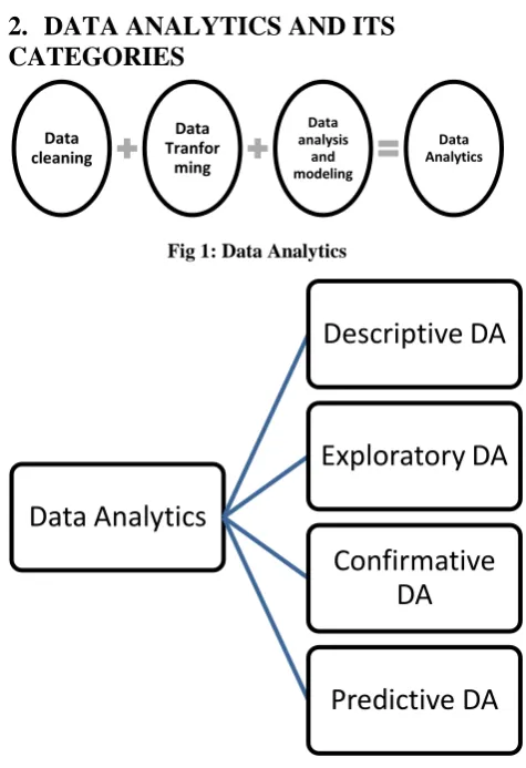
DATA ANALYTICS AND ITS
[image:1.595.312.550.190.537.2]CATEGORIES
Fig 1: Data Analytics
Fig 2: Categories of Data Analytics
3.
PROCESS FLOW
There is a step by step approach to choose a particular model for the current problem. [27] We need to decide whether a particular machine learning model is suitable for our problem or not. Here we can see process flow being followed.
Data cleaning
Data Tranfor
ming
Data analysis
and modeling
Data Analytics
Data Analytics
Descriptive DA
Exploratory DA
Confirmative
DA
Volume 179 – No.44, May 2018
Fig 3: Process of fitting a Machine Learning Model
4.
DESCRIPTION OF DATA
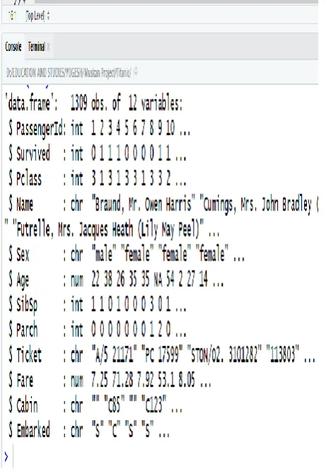
[image:2.595.309.548.81.426.2]In R str() function is used to find structure of dataset that we have in csv file. Below there is a snippet of output of we got by executing str() in R studio.
Fig 4: Structure of input Dataset
[image:2.595.55.286.376.711.2]There is table showing meaning of each attribute.
Table 1. Description of each attribute in our dataset
Attribute Description Factors
Survival Survival of
passenger 0 = No, 1 = Yes
Pclass Ticket class 1 = 1st, 2 = 2nd,
3 = 3rd
Sex Sex Male/Female
Age Age of passengers
in years
sibsp
# of siblings /
spouses aboard the Titanic
parch
# of parents /
children aboard the Titanic
ticket Ticket number
fare Passenger fare
cabin Cabin number
Embarked
Port from where passenger
embarked. C for Cherbourg, Q for Queenstown, S for Southampton
C, Q, S
Now let us explore our dataset by knowing the influence of each attribute on survival of passenger. We will create histograms, Bar plots to achieve this.
5.
DATA CLEANING
Before applying any type of data analytics on the dataset, the data is first cleaned. There are some missing values in the dataset which needs to be handled. In attributes like Age, Cabin and Embarked, missing values are replaced with random sample from existing age. [15]
In case of column Fare we found that there is one passenger with missing fare having passenger id 1044. To put a meaningful value of fair column we first found value of Embarked and Pclass of this passenger. Then median is calculated for fair values of all passenger who whose embarkation and Pclass was same as of passenger id 1044.
6.
EXPLORATORY DATA ANALYSIS
We are going to perform exploratory data analysis for our problem in the first stage. In exploratory data analysis dataset is explored to figure out the features which would influence the survival rate. The data is deeply analysed by finding a relationship between each attribute and survival.
6.1
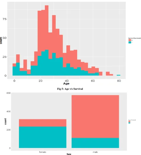
Age verses Survival
Fig 5: Age v/s Survival
Fig 6: Sex v/s Survival
[image:3.595.314.543.624.766.2]In the same way there are some more facts we found. There is a table showing age group and survival rate of that age group.
Table 2. Age Group and Survival Rate Age Group Survival Rate (%)
0-10 53.24675
10-20 38.29787
20-30 37.03704
30-40 40.21739
40-50 34.82143
50-60 34.61538
Volume 179 – No.44, May 2018
Sex verses Survival
From Fig. 6 it is clear that females are more likely to survive than males. We calculated that survival rate of female and male are 74.20382% and 18.89081% respectively.
In similar way relationship between other attributes like fare, cabin, title, family, Pclass, Embarked and survival is found. We extracted the title from attribute ‘name’. We combined parch and sibsp. In this way we will be able to decide emphasis of each attribute on survival of passenger.
7.
METHODOLOGY
7.1 Feature Engineering
Feature engineering is the most important part of data analytics process. It deals with, selecting the features that are used in training and making predictions. In feature engineering the domain knowledge is used to find features in the dataset which are helpful in building machine learning model. It helps in understanding the dataset in terms of modeling. A bad feature selection may lead to less accurate or poor predictive model. The accuracy and the predictive power depend on the choice of correct features. It filters out all the unused or redundant features.
Based on the exploratory analysis above, following features are used age, sex, cabin, title, Pclass, family size (parch plus sibsp columns), fare, embarked. Survival column is chosen as response column. These features are selected because their values have an impact on the rate of survival. These features will be the value of “x” in the bar-plots. If wrong features where selected then even the good algorithm may produce the bad predictions. Therefore, feature engineering acts like a backbone in building an accurate predictive model.
7.2 Machine Learning Models
Various machine learning models are implemented to validate and predict survival.
7.2.1 Logistic Regression
Logistic regression is the technique which works best when dependent variable is dichotomous (binary or categorical). [23] The data description and explaining the relationship between one dependent binary variable and one or more nominal, ordinal, interval or ratio-level independent variables is done with the help of logistic regression. It is used to solve binary classification problem, some of the real life examples are spam detection- predicting if an email is spam or not, health-Predicting if a given mass of tissue is benign or malignant, marketing- predicting if a given user will buy an insurance product or not.
7.2.2 Decision Tree
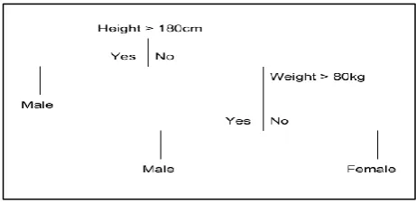
Decision tree is a supervised learning algorithm. This is generally used in problems based on classification. It is suitable for both categorical and continuous input and output variables. Each root node represents a single input variable (x) and a split point on that variable. The dependent variable (y) is present at leaf nodes. For example: Suppose there are two independent variables, i.e. input variables (x) which are height in centimeter and weight in kilograms and the task to find gender of person based on the given data. (Hypothetical example, for demonstration purpose only).
7.2.3 Random Forest
Random forest algorithm is supervised classification algorithm. The algorithm basically makes forest with large number of trees. The higher the number of trees in the forest gives the higher accuracy results. Random forest algorithm
[image:4.595.315.546.139.257.2]can be used for both classification and regression problems. For instance, it will take random samples of 100 observation and 5 randomly chosen initial variables to build a model. The same process is repeated a number of times, then the final prediction is made according to the observations. Final prediction is a function (mean) of each prediction.
Fig 7: Example of a Decision Tree
There are two types of decision tree based on the type of target variable.
1. Categorical Variable Decision Tree: The tree in which target variables have categorical values.
2. Continuous Variable Decision Tree: The tree in which the target variable has continuous values.
7.2.4 Support Vector Machine
Support Vector Machine (SVM) falls in supervised machine learning algorithm. This algorithm is used to solve both classification and regression problems. The classification is performed by constructing hyper planes in a multidimensional space that separates cases of different class labels. For categorical data variables a dummy variable is created with values as either 0 or 1. So, a categorical dependent variable consisting three levels, say (A, B, C) can be represented by a set of three dummy variables:
A: {1, 0, 0}; B: {0, 1, 0}; C: {0, 0, 1}
8.
MODEL EVALUATION
The accuracy of the model is evaluated using “confusion matrix”. A confusion matrix is a table layout that allows to visualize the correctness and the performance of an algorithm.
8.1 Confusion Matrix
A confusion matrix is a method to verify how accurately the classification model works. It gives the actual number of predictions which were correct or incorrect when compared to the actual result of the data. The matrix is of the order N*N, here N is the number of values. Performance of such models is commonly evaluated using the data in the matrix.
Sensitivity
: It defines the percentage of actual positive which are correctly identified, and is complementary to the false negative rate. Sensitivity= true positive/(true negative + false positive). The ideal value for sensitivity is “1.0” and minimum value is “0.0”Specificity:
It measures the proportion of negatives which are correctly identified, and is complementary to the false positive rate. Specificity= true negatives/(true negatives + false positives). The ideal value for specificity is “1.0” and least value is “0.0”.the sum of true positive and false positive (event that makes false prediction and subject result is also false).
Negative Predicted Value:
It is the ratio of true negatives (the event which makes negative prediction and result is also false) and sum of true negative and false negative (event that makes false prediction and subject result is positive). [image:5.595.318.535.83.227.2]8.2 Accuracy:
It gives the measure of percentage of correct prediction done by the model/algorithm. The best value is “1.0” and the worst value is “0.0”.Fig 8: Generalized confusion matrix
In R mathematical calculations are performed and accuracy using each model is found. Here are the accuracies we achieved for each model.
8.2.1 Logistic Regression
Fig 9: Confusion Matrix for Logistic Regression
In the confusion matrix the values of “a, b, c, d” gives the count of true positive, true negative, false positive and false negative respectively. The accuracy of this confusion matrix is close to “1” which shows that the model makes maximum correct predictions.
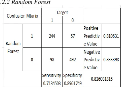
[image:5.595.317.535.195.383.2]7.2.2 Random Forest
Fig 10: Confusion Matrix for Random Forest
[image:5.595.63.273.201.303.2]7.2.3 Decision Tree
Fig 11: Confusion Matrix for Decision Tree
7.2.4 Support Vector Machine
Fig 12: Confusion Matrix for SVM
9.
PREDICTION
Here we can choose any of the models to predict survival of test sample. Since we have evaluated all models by using confusion matrix we will predict by using model which has highest accuracy.
We performed prediction on data dataset by using logistic model and SVM.
10.
GUI IMPLEMENTATION IN R
[image:5.595.58.273.362.513.2] [image:5.595.59.272.594.745.2]Volume 179 – No.44, May 2018
Fig 13: GUI Environment
11.
CONCLUSION
Data cleaning is the first step while performing data analysis. Exploratory data analytics helps one to understand the dataset and the dependency among the attributes. EDA is used to figure out the relationship between the features of the dataset. This is done by using various graphical techniques. The one used above is ggplot and histograms.
By applying EDA some conclusions are drawn and facts are found.
There is high influence of age on survival. We can see from table-2 that as age increases survival decreases.
It can be seen that survival rate of female is very high (approx. 74%) and survival rate of male is very low. This fact can also be verified by extracting titles (Mr, Mrs, Ms etc) from name column. Survival rate with title Mr. is approximately 16% while survival rate for Mrs. is 79%.
We can also see survival v/s Pclass in following table-
Table 3. Passenger Class Vs. Survival Rate Passenger class Survival Rate (%)
1 62.96296
2 47.28261
3 24.23625
We found that Passengers who were travelling in first class is more likely to survive.
We combined parch and sibsp column to know family size of a particular passenger. We found that survival rate increases when family size lies from 0 to 3. But when family size becomes greater than 3, survival rate decrease.
[image:6.595.314.542.512.654.2]Similarly it is found that passengers who has more cabins has higher survival rate.
Table 4. Passenger Class Vs. Survival Rate
Age Group Survival Rate
(0,50] 32.40223
(50,100] 65.42056
(100,150] 79.16667
(150,200] 66.66667
(200,250] 63.63636
(250,300] 66.66667
(500,550] 100
With these figure we can say that higher the fare higher will be survival rate.
In feature engineering the actual parameters to be used while designing the training model and prediction model is found out on the basis of exploratory data analytics process.
The confusion matrix gives the accuracy of all the models, the logistic regression is proves to be best among all with an accuracy of 0.837261504. This means the predictive power of logistic regression in this dataset with the chosen features is very high.
It is clearly stated that the accuracy of the models may vary when the choice of feature modelling is different. Ideally logistic regression and support vector machine are the models which give a good level of accuracy when it comes to classification problem.
12.
FUTURE WORK
This project involves implementation of data analytics and machine learning. This project work can be used as reference to learn implementation of EDA and machine learning from very basic.
In future the idea can be extended by making more advanced graphical user interface with the help of newer libraries like shiny in R. An interactive page can be made, i.e. if the value of a attribute is changed on the scale the values corresponding to its graph (ggplot or histogram) will also change. We can also draw much focused conclusions by combining results we obtained.
13.
REFERENCES
[1] Analyzing Titanic disaster using machine learning algorithms-Computing, Communication and Automation (ICCCA), 2017 International Conference on 21 December 2017, IEEE.
[2] Eric Lam, Chongxuan Tang, "Titanic Machine Learning From Disaster", LamTang-Titanic Machine Learning From Disaster, 2012.
[3] S. Cicoria, J. Sherlock, M. Muniswamaiah, L. Clarke, "Classification of Titanic Passenger Data and Chances of Surviving the Disaster", Proceedings of Student-Faculty Research Day CSIS, pp. 1-6, May 2014.
[4] Corinna Cortes, Vlasdimir Vapnik, “Support-vector networks”, Machine Learning, Volume 20, Issue 3,pp 273-297.
[5] L Breman- “random forests”, Machine Learning, 2001 Ng. CS229 Notes, Standford University, 2012.
[6] SJ Russsel P Norvig-“Artificial intelligence: A modern approach”-2016.
[7] Lonnie Stevans, David L. Gleicher, ”Who Survived the Titanic? A logistic regression analysis”-Article in International Journal of Maritime History, December 2004.
[8] MICHAEL AARON WHITLEY, Using statistical learning to predict survival of passengers on the RMS Titanic by Michael Aaron Whitley, 2015.
[9] Kunal Vyas, Zeshi Zheng, Lin Li, Titanic- Machine Learning From Disaster- 2015.
[10] EECS 349 Titanic- Machine Learning From Disaster, Xiaodong Yang, Northwestern University.
[11] Prediction of Survivors in Titanic Dataset: A Comparitive Study using Machine Learning Algorithms, Tryambak Chatterlee, IJERMT-2017.
[12] An Introduction to Logistic Regression Analysis and Reporting by Chao-Yig Joanne Peng, Kuk Lida Lee & Gary M. Ingersoll, April 2010.
[13] Zhenyan Liu, Yifei Zeng, Yida Yan, Pengfei Zhang and Yong Wang, Machine Learning for Analyzing Malware, Journal of Cyber Security and Mobility, Vol: 6 Issue: 3, July 2017.
[14] Andy Liaw and Metthew Wiener, Classification and Regression by Random Forest, vol. 2/3, December 2002. [15] Galit Shmueli and Otto R. Koppius MIS Quarterly,
Predictive Analytics in Information System Research, , Vol. 35, No. 3(September 2011), pp. 553-572.
[16] john D. Kelleher, Brain Mac Namee, Aoife D’Arcy Fundamentals of Machine Learning for Predictive Data Analytics: Algorithms .
[17] Dr. Neeraj Bhargava, Girja Sharma, Decision Tree Analysis on J48 Algorithm for Data Mining. Volume 3, Issue 6, June 2013.
[18] Data Mining: Practical Machine Learning Tools and Techniques, by Ian H. Witten, Eibe Frank, Mark A. Hall, Christopher J. Pal.
[19] A Comparison of Goodness of Fit Tests for the Logistic Regression Model, D.W. Hosmer, T. Hosmer, S. Le Cessie and S. Lemeshow
[20] Breiman, L. 2001a. Random forests. Machine Learning 45:5-32.
[21] Stuart J. Russell, Peter Norvig, Artificial Intelligence: A Modern Approach, Pearson Education, 2003, pg 697-702.
[22] Cortes, Corinna; and Vapnik, Vladimir N.; "SupportVector Networks", Machine Learning, 20, 1995. [23] Unwin A, Hofmann H (1999). \GUI and Command-line { Conict or Synergy?" In K Berk,M Pourahmadi (eds.), Computing Science and Statistics.
[24] Machine Learning Benchmarks and Random Forest Regression, Segal, Mark R, 2004.