RESEARCH ARTICLE
A CFD SIMULATION OF WATER FLOW THROUGH A VARIABLE AREA VENTURI METER
*Akpan, Patrick Udeme-obong
Department of Mechanical Engineering, University of Nigeria, Nsukka
ARTICLE INFO ABSTRACT
This work Investigates using the Ansys fluent CFD tool, the pressure difference exerted on a bluff body object and discusses the flow field from inlet to outlet. The objectives of this work are to discuss the flow field from inlet to outlet, to investigate the pressure difference exerted 25mm upstream and 25mm downstream of the bluff body object for different volumetric flow rates (4 l/s, 5 l/s and 8 l/s).The total pressure losses across the plate for the 4 l/s, 5 l/s and 8 l/s flows are 17.38 kPa, 27.14 kPa and 69.62 kPa respectively. These losses are partly due to the level of turbulence with the 8 l/s flow having the maximum turbulence intensity of over 250% exceeding those of the 4l/s and 5l/s flows which are ~130% and ~160% respectively. When compared with the mean operating pressure (101.325 kPa), these pressure losses represents 17.1%, 26.8% and 68.7% change for 4l/s 5 l/s and 8 l/s flows respectively.
Copyright © 2014 Akpan, Patrick. This is an open access article distributed under the Creative Commons Attribution License, which permits unrestricted use, distribution, and reproduction in any medium, provided the original work is properly cited.
INTRODUCTION
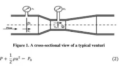
Computational Fluid Dynamics (CFD) is an aspect of fluid mechanics that utilizes numerical methods and algorithms to solve and analyze fluid flow problems (Blazek 2001; Chung 2002). The governing sets of equations which are solved include the continuity equations, Navier-Stokes equations and any additional conservation equations like energy and species concentrations. Computers are used to perform calculations required to simulate the interaction of fluids with surfaces defined by boundary conditions. A venturi meter is used to measure the volumetric flow rate ( ̇) of a fluid by making use of the venturi effect (the reduction of fluid pressure that results when fluid flows through a constricted section of pipe) (Philip et al., 2012; Morris 2001). It could also be used for mixing a liquid with a gas. This venturi effect is an outcome of applying the Bernoulli’s equation (Eq. 1) to an ideal incompressible fluid flow along a conduit surface with varying cross sectional area (see Figure.1).
+12 + = (1)
But since z is approximately constant for the two sectins (1) and (2) in Figure 1, therefore Eq. 1 becomes
*Corresponding author: Akpan, Patrick,
[image:1.595.308.562.419.561.2]Department of Mechanical Engineering, University of Nigeria, Nsukka.
Figure 1. A cross-sectional view of a typical venturi
+ 12 = (2)
Where is the total pressure made up of the static (P) and dynamic ( ) pressures. Applying the continuity equation across section (1) and (2);
̇ = (3)
And combining equations (2) and (3) we get the volumetric flow rate (see Eq. 4) at any section along the flow for an ideal flow expressed as a function of the pressure drop across the constriction lying between sections (1) and (2) along the flow.
̇ = 2( − ) − 1 =
2( − )
1 − (4)
Estimation of Permanent Pressure Loss for the flow through Obstruction type flow meters helps the selection of flow meter
ISSN: 0975-833X
International Journal of Current Research Vol. 6, Issue, 03, pp.5425-5431, March, 2014
INTERNATIONAL JOURNAL OF CURRENT RESEARCH
Article History:
Received 05thDecember, 2013 Received in revised form 10thJanuary, 2014
Accepted 14thFebruary, 2014 Published online 25thMarch, 2014
Key words: CFD Simulation, k-εTurbulence model, Ansys Fluent, Venturi meter, Water flow.
RESEARCH ARTICLE
A CFD SIMULATION OF WATER FLOW THROUGH A VARIABLE AREA VENTURI METER
*Akpan, Patrick Udeme-obong
Department of Mechanical Engineering, University of Nigeria, Nsukka
ARTICLE INFO ABSTRACT
This work Investigates using the Ansys fluent CFD tool, the pressure difference exerted on a bluff body object and discusses the flow field from inlet to outlet. The objectives of this work are to discuss the flow field from inlet to outlet, to investigate the pressure difference exerted 25mm upstream and 25mm downstream of the bluff body object for different volumetric flow rates (4 l/s, 5 l/s and 8 l/s).The total pressure losses across the plate for the 4 l/s, 5 l/s and 8 l/s flows are 17.38 kPa, 27.14 kPa and 69.62 kPa respectively. These losses are partly due to the level of turbulence with the 8 l/s flow having the maximum turbulence intensity of over 250% exceeding those of the 4l/s and 5l/s flows which are ~130% and ~160% respectively. When compared with the mean operating pressure (101.325 kPa), these pressure losses represents 17.1%, 26.8% and 68.7% change for 4l/s 5 l/s and 8 l/s flows respectively.
Copyright © 2014 Akpan, Patrick. This is an open access article distributed under the Creative Commons Attribution License, which permits unrestricted use, distribution, and reproduction in any medium, provided the original work is properly cited.
INTRODUCTION
Computational Fluid Dynamics (CFD) is an aspect of fluid mechanics that utilizes numerical methods and algorithms to solve and analyze fluid flow problems (Blazek 2001; Chung 2002). The governing sets of equations which are solved include the continuity equations, Navier-Stokes equations and any additional conservation equations like energy and species concentrations. Computers are used to perform calculations required to simulate the interaction of fluids with surfaces defined by boundary conditions. A venturi meter is used to measure the volumetric flow rate ( ̇) of a fluid by making use of the venturi effect (the reduction of fluid pressure that results when fluid flows through a constricted section of pipe) (Philip et al., 2012; Morris 2001). It could also be used for mixing a liquid with a gas. This venturi effect is an outcome of applying the Bernoulli’s equation (Eq. 1) to an ideal incompressible fluid flow along a conduit surface with varying cross sectional area (see Figure.1).
+12 + = (1)
But since z is approximately constant for the two sectins (1) and (2) in Figure 1, therefore Eq. 1 becomes
*Corresponding author: Akpan, Patrick,
Department of Mechanical Engineering, University of Nigeria, Nsukka.
Figure 1. A cross-sectional view of a typical venturi
+ 12 = (2)
Where is the total pressure made up of the static (P) and dynamic ( ) pressures. Applying the continuity equation across section (1) and (2);
̇ = (3)
And combining equations (2) and (3) we get the volumetric flow rate (see Eq. 4) at any section along the flow for an ideal flow expressed as a function of the pressure drop across the constriction lying between sections (1) and (2) along the flow.
̇ = 2( − ) − 1 =
2( − )
1 − (4)
Estimation of Permanent Pressure Loss for the flow through Obstruction type flow meters helps the selection of flow meter
ISSN: 0975-833X
International Journal of Current Research Vol. 6, Issue, 03, pp.5425-5431, March, 2014
INTERNATIONAL JOURNAL OF CURRENT RESEARCH
Article History:
Received 05thDecember, 2013 Received in revised form 10thJanuary, 2014
Accepted 14thFebruary, 2014 Published online 25thMarch, 2014
for industrial applications if the operating pressure is known. Experimental determination of permanent pressure loss is both time consuming and expensive (Durst and Wang 1989; Prajapati et al. 2010). This work is a numerical experimentation done to simulate and analyze water flow through a variable area venturi meter using a commercial computational fluid dynamics (CFD) package FLUENT. The objectives of this task are: To discuss the flow field from inlet to outlet , To investigate the pressure difference exerted 25mm upstream and 25mm downstream a bluff body object for different volumetric flow rates (4 l/s, 5 l/s and 8 l/s) and to compare the pressure difference determined from a course and fine mesh.
MATERIALS AND METHODS
Pre-Processing
Geometric Model and Meshing
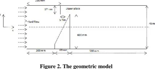
[image:2.595.305.554.348.473.2]The geometric model of the venturi meter that was modeled is shown in Figure 2. The mesh size information for both course and fine are given on Table1. The sizes of the mesh around the bluff body were made so small around the bluff body to capture adequately the physics of the flow problem.
Figure 2. The geometric model
Table 1. Mesh size information of course and fine mesh
Mesh Type
Level Cells Faces Nodes Partitions Cell Zone
Face Zone Course 0 13580 25542 11963 1 1 5 Fine 0 54118 101121 47004 1 1 5
Inlet velocity, Reynolds number and Turbulence Intensity calculation
From the flow parameters given, the inlet area, velocities, Reynolds numbers were calculated. The turbulence intensity ( ) was using Eq. 5. The turbulence intensity calculated for the 4 l/s , 5 l/s and 8 l/s flows are 3.285 % , 3.182 % and 2.976 % respectively. These are medium inlet turbulent intensity cases (Fluent Inc. 2006a).
Flow Parameters Given:
Volumetric flow rates ( ̇) = 4 l/s, 5 l/s and 8 l/s Pipe diameter ( ) = 0.078 m
Density of water (ρ) = 998.2 kg/m3
Dynamic viscosity of water ( ) = 0.001003 kg/ms
= 0.16 × (5)
Processing (Solver Execution)
In setting up the simulation, The Ansys fluent 12.1 version was launched in 2D, double precision mode. And the mesh was checked for errors. As soon as this was done, these procedures were followed:
Solver Properties and Viscous model Selection
Pressure based solver was selected. In this approach, the pressure field is extracted by solving a pressure or pressure correction equation which is obtained by manipulating the continuity and momentum equations. Steady state and absolute velocity formulation were also selected. Since a viscous incompressible flow was considered, with some turbulence intensity, the k- urbulence model based on the eddy viscosity hypothesis was selected to model the fluid flow. The decision to use this turbulence model is that it is reasonably accurate and economic in computational cost (Fluent Inc. 2006b). The solution of two additional equations by this model for the turbulent kinetic energy (TKE) ( ) and turbulent dissipation rate (TDR) ( ) in Eqs. 6 and 7 respectively is used to determine the turbulent eddy viscosity ( )in Eq. 8 which is related to the Reynolds stresses ( ′ ′) in Eq.9.
+ = + + + − (6)
+ = + + + −
(7)
= (8)
′ ′−2
3 = − + (9)
Once the Reynolds stresses are determined, they are used in the Reynolds Average Navier Stokes (RANS) equation (Eq. 10) in conjunction with the continuity equation (Eq. 11) to determine the fluid flow field.
+ = −1 + + + ( ′ ′) (10)
= 0 (11)
[image:2.595.40.291.349.460.2]gradient (Least square cells based), pressure (standard), momentum (Second order upwind), turbulent kinetic energy (second order upwind), turbulent dissipation rate (Second order upwind) The default under-relaxation factors were used: Pressure (0.3), density (1), body forces (1), momentum (0.7), and turbulent kinetic Energy (0.8), and turbulent dissipation rate (0.8), turbulent viscosity. These values are needed to stabilise the solution. The monitor check convergence criteria was set at 10-06for the residuals of continuity, x-velocity, y-velocity, k and .The solution was initialised from the inlet with reference frame relative to the cell zone. The iteration was set at 4000 times for all the flow rates including the course mesh. This is this is to ensure that all the convergence criteria were satisfied.
RESULTS AND DISCUSSION (POST PROCESSING)
The solution for the simulations carried out for the 4 l/s, 5 l/s and 8 l/s flows converged after 3390, 3383 and 3395 iterations respectively. The coarse mesh case converged after 1415 iterations. Please note that only some selected plots representing the resulting flow field are discussed in sections 3.1 -3.5.
Streamlines
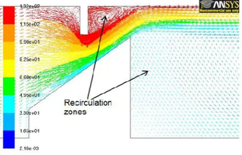
[image:3.595.311.560.104.264.2]Figures 3, 4 and 5 represents the upstream, midstream and downstream streamlines for the 5 l/s case. The flow upstream (Fig. 3) is laminar as the stream lines are in a uniform straight line. At mid-stream (Fig. 4) where turbulence is experienced, it is evident that flow separation and recirculation caused by adverse pressure difference occurs. Two recirculation zones can be seen. As the flow continued downstream (Fig. 5), the dividing streamlines reattached to the walls of the Venturi and continued until it got to the end of the flow. This same pattern was observed from the 4 l/s and 8 l/s inlet flows.
Figure 3. Upstream stream function for 5 l/s
Velocity contours and Vectors
The maximum velocity in the flow field is experienced downstream of the bluff body on the top wall surface (Fig. 6). The reduction in cross sectional area causes increase in velocity. This is also the case with the 4 l/s and 8 l/s flow rate.The maximum recirculation velocity increases in those recirculation zones with increase in volumetric flow rate. The
maximum recirculation velocity for the 4 l/s, 5 l/s and 8 l/s flow rates are – 1.92 m/s, -2.3 m/s and -3.7m/s respectively. The negative sign implies that the flow direction is reverse in the recirculation zones.
[image:3.595.43.291.472.634.2]Figure 4. Mid-stream stream function for 5 l/s
Figure 5. Downstream stream function for 5 l/s flow
Figure 6. X-Velocity vector for the 5 l/s showing details of flow around the Plate
[image:3.595.312.549.491.650.2]Pressure Contours
Figure 7. Total Pressure Contour for 5 l/s
[image:4.595.310.557.257.427.2]The maximum total pressures are 18.3 kPa, 28.5 kPa and 72.9 kPa for the 4 l/s, 5 l/s and 8 l/s flows respectively. The minimum total pressure decreased with increase in volumetric flow rate in the flow field. With the 8 l/s flow rate having the least minimum total pressure of -17.8 kPa (see Table 2).The total pressure change in the flow fields for the 4 l/s, 5 l/s and 8 l/s are 22.70 kPa, 35.46 kPa and 90.7 kPa respectively. When compared to a mean operating pressure of 101.325 kPa, the aforementioned pressure changes represents 22.4%, 35% and 89.5% change.
Table 2. Maximum and Minimum Total Pressures in the Flow fields
Flow rates (l/s)
Maximum value (kPa)
Minimum value (kPa)
Maximum Change
(kPa)
% change relative to the mean operating
pressure 4 18.300 -4.400 22.700 22.4 5 28.500 -6.900 35.460 35.0 8 72.900 -17.800 90.700 89.5
Pressure Difference across Upper Plate
Total pressure is evaluated from the summation of static and dynamic pressure (Eq. 2). , are the total pressures at 25mm upstream and downstream respectively. Each is made up of the static (P) and dynamicpressures ( ).
= + (20)
A. 25mm upstream of bluff body condition
[image:4.595.30.285.436.500.2]The total pressure profile for the different flow rates are shown on Fig.8. The total pressure for 8 l/s flow is the highest due to the fact that its flow velocity on this line is the highest (see Fig. 9). The total pressure is made up of static component mainly. The static pressure component of for the 4l/s , 5 l/s and 8 l/s flows constitutes 95.39%, 95.4% and 95.3% respectively. The maximum total pressure on at this line for the 4l/s, 5l/s and 8 l/s is shown on Table 3.
Figure 8. Total pressure 25mm upstream of upper plate
Figure 9. X-Velocity profiles at 25mm upstream of upper plate
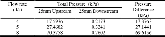
Table 3. Total Pressure (Facet Average) change across upper plate
Flow rate ( l/s)
Total Pressure (kPa) Pressure Difference
(kPa) 25mm Upstream 25mm Downstream
4 17.5936 0.2173 17.3763
5 27.4682 0.3241 27.1441
8 70.3758 0.7602 69.6156
B. 25mm downstream condition
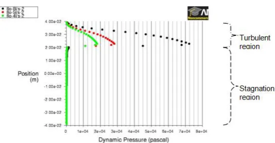
The downstream condition for the three flows has two distinct regions – the stagnation and the turbulent region. The total pressures for the flows are shown in Fig. 10. They are made up of the static and dynamic components. Stagnation region
[image:4.595.298.566.486.546.2]Figure 10. Total pressure 25mm downstream of upper plate
[image:5.595.155.439.600.748.2]Figure 11. X - Velocity 25mm downstream of the upper plate
Figure 12. Turbulence intensity at 25mm downstream of upper plate
(see Fig.12) exceeding those of the 4l/s and 5l/s flows which are ~130% and ~160% respectively. when compared with the mean operating pressure, the pressure difference represents 17.1% , 26.8% and 68.7% change for the 4 l/s , 5 l/s and 8 l/s flows respectively.
Pressure Difference across upper Plate (Course versus Fine Mesh)
[image:6.595.306.558.80.123.2]The graphical representation of the total pressures 25mm upstream and downstream for the coarse and fine mesh used for the 5 l/s are shown on Fig. 14 and 15 respectively. The upstream section shows different profiles for the upstream pressures for the coarse and fine mesh (see Fig. 14). Table 4 shows the computed values for the total pressures for both meshes. The difference between the computed total pressure difference across the upper plate for the coarse and fine mesh is 0.464 kPa which represents 1.68 % increment over the fine mesh result. This implies that our solution for the coarse mesh is grid independent considering the fact that with ~299 % increase in number of cells from 13,580 cells (coarse grid) to 54,118 cells (fine grid), only 1.68% change was obtained in pressure difference. Within 1.68% error limit, the solutions from the coarse mesh could relied on , hence the reduction in the computational cost of using the fine mesh.
[image:6.595.44.289.354.525.2]Figure 14. Total pressure 25mm upstream for Coarse and Fine mesh (5 l/s flow)
Figure 15. Total Pressure 25mm downstream for coarse and fine mesh (5 l/s flow)
Table 4. Total Pressure (Facet Average) 25mm upstream and downstream for 5 l/s Flow
Mesh Total pressure (kPa) Difference (kPa)Pressure 25mm upstream 25mm downstream
Fine 27.4681 0.3241 27.144 Coarse 27.8777 0.2697 27.608
Conclusion
The numerical experimentation carried out in this study, to simulate the flow of water in a variable area venture meter using the commercially available CFD package Ansys fluent 12.0 version has shown that the pressure drop 25mm upstream and downstream of the upper plate is proportional the volumetric flow rate across the plate. This proportionality is not linear. The total pressure drop across the plate for the 4 l/s, 5 l/s and 8 l/s flows are 17.38 kPa, 27.14 kPa and 69.62 kPa respectively. The losses in pressure across the plate are partly due to the level of turbulence (over 250%), which exceeds the values for the 4l/s and 5l/s flows which are ~130% and 160% respectively (see Fig. 12). When compared with the mean operating pressure (101.325 kPa), these pressure losses across the vertical plate represents 17.1%, 26.8% and 68.7% change for 4l/s and 5l/s flow situations. The difference between the computed total pressure difference for the coarse and fine mesh is 0.464 kPa. This represents 1.68 % increment over the fine mesh result. Within a reasonable error limit of 1.68% the results of the coarse mesh could be relied on, thus saving computational cost. Though results obtained in this work may not be relied on 100% because of the errors associated with the modelling, discretisation and iteration, it could serve as a good starting point for further study.
Nomenclatures
Symbol Definition Unit
Area [m2]
Pipe diameter [m]
Force per unit mass [m/ s2] Acceleration due to gravity [m/s2] Turbulence Intensity [%] Turbulent kinetic energy [m2/s2]
Static pressure [m2] Total Pressure [N/ m2]
Density [kg/m3]
Time [s]
Velocity [m/s]
Kinematic viscosity [m2/s]
̇ Volumetric flow rate [m /s]
Displacement [m]
Elevation [m]
Dynamic viscosity [kg/ms] Turbulent eddy viscosity [m2/s] Turbulent dissipation rate [m2/s3] Turbulent kinetic energy Prandtl Number [-] Turbulent dissipation rate Prandtl number [-] Subscripts
1 upstream 2 downstream
[image:6.595.43.290.559.732.2]Acknowledgement
The author wishes to specially appreciate Esso-Exploration and Production Nigeria Limited (EEPNL) for sponsoring my MSc programme at Cranfield University, UK where I got the opportunity to use the computational resources of the Applied Mathematics and Computing group, Cranfield University, UK for this research work.
REFERENCES
Blazek, J. 2001. Computational fluid dynamics: principles and applications. Elsevier Science, Oxford.
Chung, T. J. 2002. Computational fluid dynamics.Cambridge University Press, Cambridge.
Durst, F. and Wang, A.B. 1989. Experimental and numerical investigation of the axisymmetric, turbulent pipe flow over a wall- mounted thin obstacle, Seventh Symposium on Turbulent Shear Flows, Stanford University, 21-23 August Fluent Inc. 2006a. Fluent 6.3 user guide documentation. Fluent
Inc., Lebanon.
Fluent Inc. 2006b. Fluent 6.3 tutorial guide documentation. Fluent Inc., Lebanon.
Morris A. S. 2001. Measurement and instrumentation principles. Butterworth-Heinemann publishers, oxford. Patankar, S. V. and Spalding, D. B. 1972. A calculation
procedure for heat, mass and momentum transfer in three-dimensional parabolic flows. International J. Heat and Mass Transfer, 15, 1787.
Philip J, Sharma A., Jain N., and Nithin T. 2012. “Optimization of venturi flow meter model for the angle of divergence with minimal pressure drop by computational fluid dynamics method international conference on recent development in engineering and technology, 5th august, Mysore, ISBN-978-93-82208-00-6.
Prajapati C. B., Patel V.K., Singh S.N. and Seshadri V. 2010. CFD analysis of permanent pressure loss for different types of flow meters in industrial applications: Proceedings of the 37th National and 4th International Conference on Fluid Mechanics and Fluid Power December 16-18, 2010, IIT Madras, Chennai, India.