Deep Video Precoding

Deep Video Precoding

Eirina Bourtsoulatze, Aaron Chadha, Ilya Fadeev, Vasileios Giotsas, and Yiannis Andreopoulos

Abstract—Several groups worldwide are currently investigating how deep learning may advance the state-of-the-art in image and video coding. An open question is how to make deep neural networks work in conjunction with existing (and upcoming) video codecs, such as MPEG H.264/AVC, H.265/HEVC, VVC, Google VP9 and AOMedia AV1, as well as existing container and transport formats, without imposing any changes at the client side. Such compatibility is a crucial aspect when it comes to practical deployment, especially when considering the fact that the video content industry and hardware manufacturers are expected to remain committed to supporting these standards for the foreseeable future.

We propose to use deep neural networks as precoders for current and future video codecs and adaptive video streaming systems. In our current design, the core precoding component comprises a cascaded structure of downscaling neural networks that operates during video encoding, prior to transmission. This is coupled with a precoding mode selection algorithm for each independently-decodable stream segment, which adjusts the downscaling factor according to scene characteristics, the utilized encoder, and the desired bitrate and encoding configuration. Our framework is compatible with all current and future codec and transport standards, as our deep precoding network structure is trained in conjunction with linear upscaling filters (e.g., the bilinear filter), which are supported by all web video players. Results with FHD (1080p) and UHD (2160p) content and widely-used H.264/AVC, H.265/HEVC and VP9 encoders show that coupling such standards with the proposed deep video precoding allows for 15% to 45% rate reduction under encoding con-figurations and bitrates suitable for video-on-demand adaptive streaming systems. The use of precoding can also lead to encoding complexity reduction, which is essential for cost-effective cloud deployment of complex encoders like H.265/HEVC and VP9, especially when considering the prominence of high-resolution adaptive video streaming.

Index Terms—video coding, neural networks, downscaling, upscaling, adaptive streaming, DASH/HLS

I. INTRODUCTION

I

and NOW TV than to traditional pay TV services.1 The

proliferation of over-the-top (OTT) streaming content has been matched by an appetite for high-resolution content. For example, 50% of the US homes will have UHD/4K TVs by 2020. At the same time, costs of 4K camera equipment have been falling rapidly. Looking ahead, 8K TVs were introduced at the 2018 CES by several major manufacturers and several broadcasters announced they will begin 8K broadcasts in time for the 2020 Olympic games in Japan. Alas, for most countries,

All authors are with iSIZE Ltd., 3 Falconet Court, 123 Wapping High Street, London, E1W 3NX, United Kingdom, email: [email protected].

1

https://www.ofcom.org.uk/about-ofcom/latest/media/media-releases/2018/streaming-overtakes-pay-tv

even the delivery of FHD (1080p) content is still plagued by broadband infrastructure problems.

To get round this problem, OTT content providers resort to adaptive streaming technologies, such as Dynamic Adaptive Streaming over HTTP (DASH) and HTTP Live Streaming (HLS), where the streaming server is offering bitrate/resolution ladders via the so-called “manifest” file [1], [2]. This allows the client device to switch to a range of lower resolutions and bitrates when the connection bandwidth does not suf-fice to support the high-quality/full-resolution video bitstream [1]. In order to produce the bitrate/resolution ladders, high-resolution frames are downscaled to lower high-resolutions, with the frame dimensions being reduced with decreased bitrate. Within all current adaptive streaming systems, this is done using standard downscaling filters, such as the bicubic filter, and the chosen resolution per bitrate stays constant throughout the content’s duration and is indicated in the manifest file. At the client side, if the chosen bitrate corresponds to low-resolution frames, these frames are upscaled after decoding to match the resolution capabilities of the client’s device. Unfortunately, the impact on visual quality from the widely-used bicubic downscaling and the lack of dynamic resolution adaptation per bitrate can be quite severe [3]. In principle, this could be remedied by post-decoding learnable video upscaling solutions similar to learnable super-resolution techniques for still images [4], [5]. However, their deployment requires substantial changes to the client device, which are usually too cumbersome and complex to make in practice (a.k.a., the hidden technical debt of machine learning [6]). For example, convolutional neural network (CNN) based upscalers with tens of millions of parameters cannot be supported by mainstream CPU-based web browsers that support DASH and HLS video playback.

A. Precoding for Video Communications

Precoding has been initially proposed for MIMO wireless communications as the means to preprocess the transmitted symbols and perform transmit diversity [7]. Precoding is similar to channel equalization, but the key difference is that one has to optimize the precoder with the operation of the utilized receiver. While channel equalization aims to minimize channel errors, a precoder aims to minimize the error in the receiver output.

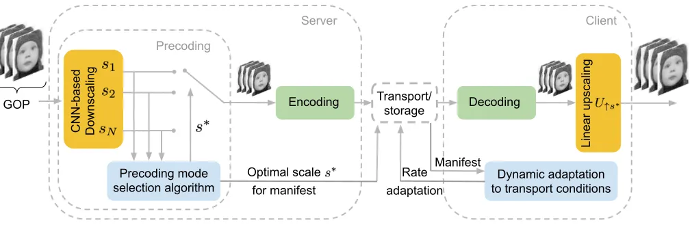
In this paper, we introduce the concept of precoding for adaptive video streaming. As illustrated in Fig. 1, precoding for video is done by preprocessing the input video frames of each independently-decodable group of pictures (GOP) prior to standard encoding, while allowing a standard video decoder and player to decode and display them without requiring any modifications. The key idea of precoding is to minimize the

CNN-based _Downscaling

Precoding mode selection algorithm

Encoding Transport/ Decoding

storage GOP

Linear upscaling

Precoding

Server Client

Dynamic adaptation to transport conditions Optimal scale

for manifest

Rate adaptation

Manifest

Fig. 1. Proposed deep video precoding framework. The precoding module performs dynamic resolution adaptation during encoding, prior to streaming. The optimal scale factor is chosen by our adaptive precoding mode selection algorithm which operates per GOP, bitrate and codec and is passed to the server-based manifest file that points all adaptive streaming clients to the available content chunks (GOPs) and their bitrate and resolution settings.

distortion at the output of the client’s player. To achieve this, we leverage on the support for multiple resolutions at the player side and introduce a multi-scale precoding convolu-tional neural network (CNN) that progressively downscales input high-resolution frames over multiple scale factors. A mode selection algorithm then selects the best precoding mode (i.e., resolution) to use per GOP based on the GOP frame content, bitrate and codec characteristics. The precoding CNN is designed to compact information in such a way that the aliasing and blurring artifacts generated during linear upscaling are mitigated. This is because, in the vast majority of devices, video upscaling is performed by means of linear filters. Thus, our proposed deep video precoding solution focuses on matching standard video players’ built-in linear upscaling filter implementations, such as the bilinear filter2_.

Our experiments with standard FHD (1080p) and UHD (2160p) test content from the XIPH repository and well-established implementations of H.264/AVC, H.265/HEVC and VP9 encoders show that, by using deep precoding modes for downscaling, we can significantly reduce the distortion of video playback compared to conventional downscaling filters and fixed downscaling modes used in standard DASH/HLS streaming systems. We further demonstrate through extensive experimentation that the proposed adaptive precoding mode selection achieves 15%-45% bitrate reduction for FHD and UHD content encoding at typical bitrate ranges used in com-mercial deployments. An important effect of the proposed precoding is that video encoding can be accelerated, since many GOPs tend to be shrunk by the precoder to only 6%-64% of their original size, depending on the selected downscaling factor. This is beneficial when considering cloud deployments

2_{Despite an abundance of possible upscaling filters, in order to remain}

effi-cient over a multitude of client devices, most web browsers only support the bilinear filter for image and video upscaling in YUV colorspace, e.g., see the Chromium source code that uses libyuv, https://chromium.googlesource.com.

of such encoders, especially, in view of upcoming standards with increased encoding complexity.

In summary, our contributions are as follows:

• the concept of deep precoding for video delivery is intro-duced as the means of enhancement of the rate-distortion characteristics of any video codec without requiring any changes on the client/decoder side;

• a multi-scale precoding CNN is proposed, which

down-scales high-resolution frames over multiple scale factors and is trained to mitigate the aliasing and blurring arti-facts generated by standard linear upscaling filters;

• an adaptive precoding mode selection algorithm is

pro-posed, which adaptively selects the optimal resolution prior to encoding.

precoding is done in its entirety during content encoding and remains agnostic to the transport conditions experienced during each individual video bitstream delivery.

B. Paper Organization

The remainder of this paper is organized as follows. In Sec. II, we review related work. The proposed multi-scale deep precoding network architecture design, loss function, and implementation and training details are presented in Sec. III. The precoding mode selection is presented in Sec. IV. Exper-imental results are given in Sec. V, and Sec. VI concludes the paper.

II. RELATED WORK

Content-adaptive encoding has emerged as a popular solu-tion for quality or bitrate gains in standards-based video en-coding. Most commercial providers have already demonstrated content-adaptive encoding solutions, typically in the form of bitrate adaptation based on combinations of perceptual metrics, i.e., lowering the encoding bitrate for scenes that are deemed to be simple enough for a standard encoder to process. Such solutions can also be extended to other encoder parameter adaptations, and their essence is in the coupling of a visual quality profile to a pre-cooked encoder-specific tuning recipe. More broadly, resolution adaptation in image and video coding has been explored by several authors. Starting from non-learnable designs, Tsaig et al. [8] explored the design of optimal decimation and interpolation filters for block image coders like JPEG and showed that low-bitrate image coding between 0.05 bits-per-pixel (bpp) to 0.35 bpp benefits from such designs. Georgis et al. [9] proposed backprojection-based upscaling that is tailored to Gaussian kernel downscaling and showed that such approaches can be beneficial for FHD and UHD/4K encoding with H.264/AVC and HEVC up to 10mbps and 5mbps, respectively. Kopfet al. [10] proposed a content-adaptive method, wherein filter kernel coefficients are adapted with respect to image content. Oztireli et al. [11] proposed an optimization framework to minimize structural similarity between the nearest-neighbor upsampled low-resolution image and the high-resolution image. Recently, Katsavounidiset al. [3], [12] proposed the notion of the dynamic optimizer in video encoding: each scene is downscaled to a range of resolutions and is subsequently compressed to a range of bitrates. After upscaling to full resolution, the convex hull of bitrates/qualities is produced in order to select the best operating resolution for each video segment. Quality can be measured with a wide range of metrics, ranging from simple peak signal to noise ratio (PSNR) to complex fusion-based metrics like the video multimethod assessment fusion (VMAF) metric [13]. While Bjontegaard distortion-rate (BD-rate) [14] gains of 30% have been shown in experiments for H.264/AVC and VP9, the dynamic optimizer requires very significant computational resources, while it still uses non-learnable downscaling filters. Overall, while such methods have shown the possibility of rate saving via image and video downscaling, they have not managed to outperform classical bicubic downscaling within the context of practical encoding. This has led most researchers

and practitioners to conclude that downscaling with bicubic or Lanczos filters is the best approach, and instead the focus has shifted on upscaling solutions at the client (i.e., decoder) side that learn to recover image detail assuming such downscaling operators. This shift has been largely fuelled by the success of deep CNN architectures for single image super-resolution, that have set the state-of-the-art, with recent architectures like VDSR [15], EDSR [16], FSRCNN [17], DRCN [18] and DBPN [4] achieving several dB higher PSNR in the luminance channel of standard image benchmarks for lossless image upscaling. Thus, Afonsoet al.propose a spatio-temporal reso-lution adaptation where a CNN-based super-resoreso-lution model is used to reconstruct full-resolution content [19]. Liet al.[20] introduce the block adaptive resolution coding framework for intra frame coding, where each block within a frame is either downscaled or coded at original resolution and then upscaled with a trained CNN at the decoder side. This concept was later extended to include P and B frames as well [21]. Differently from the previous methods that operate in the pixel domain, Liuet al.perform down and upsampling in the residue domain and design upsampling CNN for residue super resolution (SR) with the help of the motion compensated prediction signal [22]. However, regardless of the domain where they operate, the common principle of all these works is that they use hand-crafted filters for downscaling and perform upscaling at the decoder side using codec-tailored CNN models integrated in the coding standard which requires modifications to the codec. While most research efforts have focused on learning optimal upscaling filters [23], inspired by the success of autoencoders for image compression [24], [25], some recent works revise the problem of joint downscaling and upscaling using deep CNN-based methods. Shocheret al.[26] recently proposed an upscaling method using deep learning, which trains an image-specific CNN with high and low-resolution pairs of patches extracted from the test image itself. Weberet al.[27] used convolutional filters to preserve important visual details, and Houet al.[28] recently proposed a deep perceptual loss based method. Kimet al.[29] proposed an image down-scaling/upscaling method using a deep convolutional autoen-coder, and achieved state-of-the-art results on standard image benchmarks. An end-to-end image compression framework for low bitrates compatible with existing image coding standards is introduced in [30]. It comprises two CNNs: one for image compaction prior to encoding and one for post-processing after decoding. Adaptive spatio-temporal decomposition prior to encoding, followed by CNN-based spatio-temporal upscaling

after decoding has been proposed by Afonso et al. and was

side that cannot be supported by existing video players as they break away from current standards. Therefore, despite the significant advances that may be offered by all these methods in their future incarnations, they do not consider the stringent complexity and standards compatibility constraints imposed when dealing with adaptive video streaming under DASH or HLS-compliant clients like web browsers. Our work fills this gap by offering deep video precoding as the means to optimize existing video encoders with the entirety of the precoding process taking place on the server side and not requiring any change in the video transport, decoding and display side.

III. MULTI-SCALE PRECODING NETWORKS

While any downscaling method can be used with the video precoding framework of Fig. 1, to enhance the performance of our proposal in a data-driven manner, we introduce a multi-scale precoding neural network. The precoding network comprises a series of CNN precoding blocks that progressively downscale high resolution (HR) video frames over multiple scale factors. We design the precoding CNN to compact information such that a standard linear upscaler at the video player side will be able to recover in the best possible way. This is the complete opposite of recent image upscaling architectures that assume simple bicubic downscaling and an extremely complex super-resolution CNN architecture at the video player side. For example, EDSR [5] comprises over 40 million parameters and would be highly impractical on the client side for 30-60 frame-per-second (fps) FHD/UHD video. In the following subsections, we describe the design of the proposed multi-scale precoding networks, including the net-work architecture, loss function, and details of implementation and training.

A. Network Architecture

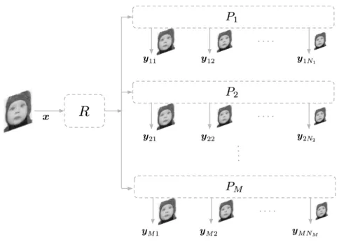
The overall architecture of the precoding network is

de-picted in Fig. 2. It consists of a “root” mapping R

fol-lowed by M parallelized precoding streams Pm. The

net-work progressively downscales individual luminance frames

x ∈ RH×W(where H and W are the height and width,

respectively) over the scale factors in S. Considering that the human eye is most sensitive to luma information, we intentionally process only the luminance (Y) channel with the precoding network and not the chrominance (Cb, Cr) channels, in order to avoid unnecessary computation. Dong et al. [34] support this claim empirically and, additionally, find that training a network on all three channels can actually worsen performance due to the network falling into a bad local minimum. We also note that this permits for chroma subsampling (e.g., YUV420) as the chrominance channels (Cb,Cr) are downscaled independently using the standard bicubic filter.

1) Root mapping: The root mappingR, illustrated in Fig 3, comprises two convolutional layers and extracts a set of

high-dimensional feature maps r ∈ RH×W×K from the inputx,

whereKis the number of output channels of the root mapping. The root mappingRconstitutes less abstract features (such as edges) that are common amongst all precoding streams and

Fig. 2. The architecture of our multi-scale precoding network for video down-scaling, comprising a root mappingRand precoding streamsP1, P2, . . . PM.

The luminance frame of each input video frame is downsampled to multiple lower resolutions by the precoding network at the server via the precoding streams.

Fig. 3. Root mappingRandm-th precoding streamPm. The root mapping

extracts high-dimensional feature maps r and is shared by all precoding streams. The precoding streamPmcontains a sequence of precoding blocks

and progressively downsamples the input high-resolution frames over a set of Nmscale factors.

scale factors. Therefore, this module is shared between all precoding streams, which helps in reducing complexity.

2) Precoding stream: The extracted feature maps r are passed to the precoding streams. As depicted in Fig. 3, a

precoding streamPmcomprises a sequence ofNmprecoding

blocks, which progressively downscale the input over a subset of Nm scale factors, Sm = {sm1, sm2, . . . , smNm} ⊆ S, where 1 < sm1 < sm2 < · · · < smNm. The allocation of scale factors to a precoding stream is done in such a way that: (i)complexity is shared equally between streams for efficient parallel processing and(ii)the ratio of most of the consecutive pairs of scalessm(n−1), smn within a stream is constant, i.e.,

αmn = smn/sm(n−1) = αm ∈ Z+. Such construction of

Fig. 4. Precoding block design, comprising a series of 3×3 and 1×1 convolutions. The linear downscaling operation D↓αmn is only performed

when the downscaling to the target resolution cannot be achieved via stride in the first convolutional layer. The linear mapping learned from the first layer (pre-activation function) is passed to the output of the second3×3 convolutional layer (post-activation function) with a skip connection and pixel-wise summation.

similar scales and enables parameter sharing within each precoding stream, thus further reducing the computational complexity. Most importantly, it renders our network amenable to standard encoding resolution ladders, such as those used in DASH/HLS streaming [2].

Given a precoding streamPm, then-th constituent

precod-ing block receives a function of the output map pm(n−1) ∈

RH/sm(n−1)×W/sm(n−1)×K _{from the preceding block and}

out-puts embedding pmn ∈ RH/smn×W/smn×K_{. Notably, we}

utilize a global residual learning strategy, where we use a skip connection and perform a pixel-wise summation between the root feature maps r (pre-activation function and after linear downscaling to the correct resolution with a linear downscaling operator D↓smn) and pmn. Similar global residual learning implementations have also been adopted by SR models [35]– [37]. In our case, our precoding stream effectively follows a pre-activation configuration [38] without batch normaliza-tion. We find empirically that convergence during training is generally faster with global residual learning, as the precoding blocks only have to learn the residual map to remove distortion introduced by downscaling operations.

The resulting downscaled feature map is finally mapped by a single convolutional layer Fmn to ymn. Importantly,

the sequence of precoding blocks only operates in a higher dimensional feature space without any heavy bottlenecks. It is then the job of convolutional layers Fmn to aggregate block outputs into single channel representations of the input x,

downscaled by a factor of smn. For Nm precoding blocks

and set of Nm scale factors Sm, the embedding stream

outputs a set ofNmcorresponding downscaled representations Ym={ym1,ym2, . . . ,ymNm} of the inputx.

The output activations inYmare clipped (rescaled) between

the minimum and maximum pixel intensities and each repre-sentation can, thus, be passed to the codec as a downscaled low resolution (LR) frame. These frames can then be individually upscaled to the original resolution using a linear upscaling

U↑s on the client side, such as bilinear, lanczos or bicubic,

where ↑s indicates upscaling by scale factor s. We refer to the upscaled frame generated from the downscaled frameymn

as xˆmnand denote the set ofNmupscaled representations of

x asXˆm={xˆm1,xˆm2, . . . ,xˆmNm}.

3) Precoding block: Our precoding block, which consti-tutes the primary component of our network, is illustrated in

Fig. 4. The precoding block consists of alternating 3×3 and 1×1convolutional layers, where each layer is followed by a parametric ReLU (PReLU) [39] activation function. The1×1 convolution is used as an efficient means for channel reduction in order to reduce the overall number of multiply-accumulates (MACs) for computation.

The n-th precoding block in the m-th precoding stream

is effectively responsible for downscaling the original high resolution frame by a factor ofsmn. In order to maintain low

complexity, it is important to downscale to the target resolution as early as possible. Therefore, we group all downsampling operations with the first convolutional layer in each precoding block. Denoting the input to the precoding block asimn, the

output of the first convolutional layer Cmn of the precoding block ascmn (as labelled in Figure 4) and spatial stride ask:

cmn=

(

Cmn(imn;k=αmn), ifαmn∈Z+ Cmn(D↓αmn(imn);k= 1), otherwise

(1)

In other words, downscaling is implemented in the first convolutional layer with a stride if αmn is an integer; other-wise we use a preceding linear downscaling operationD↓αmn (bilinear or bicubic).

The aim of the precoding block is to reduce aliasing artifacts in a data-driven manner. Considering that the upscaling opera-tions are linear and, therefore, heavily constrained, the network is asymmetric and the precoding structure can not simply learn to pseudo invert the upscaling. If that were to be the case, it would simply result in a traditional linear anti-aliasing filter, i.e., a lowpass filter that removes the high frequency components of the image in a globally-tuned manner, such that the image can be properly resolved. Removing the high fre-quencies from the image leads to blurring. Adaptive deblurring is an inverse problem, as there is typically limited information in the blurred image to uniquely determine a viable input. As such, within our proposed precoding structure, we can respectively model the anti-aliasing and deblurring processes as a function composition of linear and non-linear mappings. As illustrated in Fig. 4, this is implemented with a skip connection between linear and non-linear paths, as utilized in ResNet [40] and its variants, again following the pre-activation structure. In order to ensure that the output of the non-linear path has full range (−∞,∞), we can initialize the final PReLu before the skip connection such that it approximates an identity function.

B. Loss Function

Given the luminance channel of a ground-truth frame x∈

RH×W (with Y ranging between 16-235 as per ITU-R BT.601

conversion), our goal is to learn the parameters for the root

R and all precoding streams P1, P2, . . . PM. We denote the root module parameters as θ and the parameters of the m-th precoding stream asφm. For them-th precoding stream with

Lm( ˆXm,x;θ,φm) =

1

I I

X

i=1

Nm X

n=1

xˆ

(i)

mn−x(i)

+λ

∇xˆ

(i)

mn− ∇x

(i)

(2)

The first term represents the L1 loss between each generated upscaled frame xˆmn = U↑smn(ymn) and the ground-truth

frame x, summed over all Nm scales, whereymn=Fm,n◦

Pm,↓s_mn ◦R(x;θ,φm) and Pm,↓smn is the part of the m -th precoding stream -that includes all precoding blocks up to the n-th block and is responsible for downscaling the input

feature maps r by the scale factor smn. The second term

represents the L1 loss between the first order derivatives of the generated high resolution and ground-truth frames. As the first order derivatives correspond to edge extraction, the second term acts as an edge preservation regularization for improving perceptual quality. We set the weight coefficient

λ to 0.5 for all experiments; empirically, this was found to produce the best visual quality in output frames. Contrary to recent work [29], we do not add a loss function constraint between the downscaling and upscaling as our upscaling is only linear and, therefore, already heavily constrains the downscaled frames. Most importantly, we do not include the codec in the training process and train end-to-end (i.e., without encoding/transcoding), such that the model does not learn codec specific dependencies and is able to generalize to mul-tiple codecs. Finally, as we train the parallelized multi-scale precoding network over all streams synchronously, our final loss function is the summation of (2) over all M precoding streams:

L( ˆX,x;θ,φ) =

M

X

m=1

Lm( ˆXm,x;θ,φm) (3)

whereXˆ = ˆX1∪Xˆ2∪· · ·∪XˆM andφ={φ1,φ2, . . . ,φM}.

C. Implementation and Training Details

In our proposed multi-scale precoding network, we initialize all kernels using the method of Xavier intialization [41]. We use PReLU as the activation function, as indicated in Fig. 3 and 4. We use zero padding to ensure that all layers are the same size and downscaling is only controlled by a downsampling operation such as a stride or a linear downscaling filter.

The root mapping R comprises a single 3 ×3 and 1 ×1

convolutional layers. We set the number of channels in all 1×1 and3×3 convolutional layers to 4 and 8, respectively (excluding Fm,n, which uses a kernel size of 3×3 but with

only a single output channel).

Our final parallelized implementation comprises three pre-coding streams P1, P2 and P3, with the set of scale factors

S \ {1} partitioned into three subsets: S1 = {4/3,2,4},

S2 = {3/2,3,6} and S3 = {5/4,5/2}. Collectively, these include all representative scale factors used in DASH/HLS streaming systems [2], as well as additional scale factors that offer higher flexibility in our adaptive mode selection algorithm. In terms of complexity, for a 1920×1080×4 -dimensional feature map (assuming no downscaling), a single

precoding block requires approximately only 1.33G MACs for downscaling and 640 parameters. Our final implementation requires only 3.38G MACs and 5.5K parameters over all scales for an FHD input frame (1920×1080), including root mapping and all precoding streams.

We train the root module and all precoding streams end-to-end with linear upscaling, without the codec, on images from the DIV2K [42] training set. We train all models with the Adam optimizer with a batch size of 32 for 200k iterations. The initial learning rate is set as 0.001 and decayed by a factor of 0.1 at 100k iterations. We use data augmentation during training, by randomly flipping the images and train with a

120×120 random crops extracted from the DIV2K images.

All experiments were conducted in Tensorflow on NVIDIA K80 GPUs. We do not use Tensorflow’s built-in linear image resizing functions and rewrite all linear upscaling/downscaling functions from scratch, such that they match standard FFmpeg and OpenCV implementations.

IV. ADAPTIVE VIDEO PRECODING

Given the trained multi-scale precoding network, the mode selection algorithm operates on a per GOP, bitrate and codec basis. The goal of mode selection is to determine the optimal precoding scale factor for each GOP. While one can use operational rate-distortion (RD) models for H.264/AVC or H.265/HEVC [43] for evaluation of the best precoding modes, such models cannot encapsulate the complex and sequence-dependent RD behavior of each codec preset. On the other hand, exhaustive search solutions like the Netflix dynamic optimizer [3] require numerous highly-complex encodings per bitrate and scale factor. This makes them impractical for high-volume/low-cost encoding systems. Our approach provides a middle ground between these two opposites by computing operational rate-distortion characteristics of the video encoder for each precoding mode and video segment in an efficient manner.

The precoding mode selection algorithm is outlined in Algorithm 1 and comprises three steps. The first step is to obtain the rate-distortion characteristics of each precoding mode (scale). LetS={s1, s2, . . . , sN}be the complete set of

scale factors that may include the native (i.e., full) resolution. Each GOP segment g is precoded into all possible scales in S with the multi-scale precoding network. Lethi denote the

precoded version of GOP g using scale factor si ∈ S. All

precoded versions of GOPg are then encoded with the video encoder’s preset and encoding parameters. As such, per scale

factor si, we obtain a single GOP encoding, which, after

decoding and upscaling to the native resolution, produces a single rate-distortion point (Ri, Di) on the RD plane.3 _This

provides significant reduction of the required encodings versus approaches like the Netflix dynamic optimizer, which needs a convex hull of several rate-distortion points per scale factor

si, i.e., several encodings per scale factor [3]. To accelerate this step even further and avoid unnecessary computational

3_{We use mean squared error (MSE) to measure distortion. Even though}

overhead, we introduce a “footprinting” process: instead of encoding all frames of the GOP, we perform selective encoding of only a few frames, e.g., keeping only every n-th frame in the GOP. This significantly speeds up the initial encoding step, especially if multiple precoding modes are considered, as n

times fewer frames need to be precoded and encoded per scale factor. We store the set of tuplesR={(Ri, Di,hi, si)}|S|_i=1.

Once all the RD points are obtained, we start the pruning process. First, we eliminate all precoding modes, whose RD points do not provide for a monotonically decreasing RD curve. That is, for every precoding mode i, if there exists a precoding modej, such thatRj≤Ri andDj < Di, thesi

precoding mode is pruned out. If, after this elimination pro-cedure, the number of remaining precoding modes is greater than two, we further prune out precoding modes by eliminating those modes whose RD points do not lie on the convex hull of the remaining RD points [44], [3]. We refer to the set of pruned tuples asRpruned⊆R. After the pruning stage, we re-encode the remaining precoded GOP representationshi using

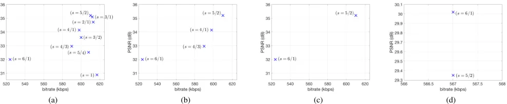
constant bitrate (CBR) encoding. The bitrate used for the CBR encoding is equal to the average of the bitrates of all RD points remaining after the elimination step. After decoding and upscaling to the native resolution, we obtain a new set of tuples,R_pruned0 , corresponding to the CBR encoding. This final step of the algorithm essentially remaps the RD points that remain after the pruning process to a common bitrate value, which is enforced by the CBR encoding. The optimal precoding modes∗is then selected as the mode providing the lowest distortion among this new set of remapped RD points. For illustration purposes, we demonstrate in Fig. 5a-5d the operation of the mode selection algorithm on the first

GOP (first 30 frames) of the aspen FHD sequence when

the latter is encoded with H.264/AVC with target bitrate set to 500kbps. For downscaling, we use nine scale factors S ={1,5/4,4/3,3/2,2,5/2,3,4,6} with our trained multi-scale precoding network (described in Section III), while upscaling is performed using the bilinear filter. Fig. 5a shows the set of RD points obtained after precoding the GOP for

each scale factor in S and encoding with H.264/AVC via

VBV encoding with the CRF values of Table I, which is representative of real-world streaming presets [33], and both maximum bitrate and buffer size set to 500kbps. As shown in Fig. 5b, the RD points (and the corresponding precoding modes) that do not provide for a monotonically increasing rate-PSNR curve are eliminated from the RD plane. Since there are more than two points remaining after this step, we next prune out the points that do not lie on the convex hull,

which leaves us with two candidate precoding modes s= 6

and s = 5/2. We finally re-encode the GOP, precoded with the two modes, with CBR encoding at 567kbps, which is the average bitrate of the two points in Fig. 5c. This results in the two RD points shown in Fig. 5d. The selected precoding mode is s∗ = 6, since it renders the highest PSNR value between the two points. Notice that the CBR encoding acts as an RD remapping and leads to both modes obtaining lower PSNR values than their PSNRs under VBV encoding. However, the absolute PSNR values are not relevant, since we are looking for the maximum PSNR under CBR; the final precoding mode

is applied on the entire GOP and the encoding uses the VBV encoding mode preset. Finally, it is also of interest to notice that for this low-bitrate case, thes= 1case (full resolution) is immediately shown to be suboptimal, and the mode selection is left to select from the higher-quality/higher-bitrate mode of

s = 5/2 and the lower-quality/lower-bitrate mode of s = 6, with the latter prevailing when remapping the two points into CBR encoding at their average rate.

Algorithm 1 : Algorithm for adaptive mode selection Input: GOP segmentg, complete set of scale factorsS Output: optimal precoding modes∗, optimal precoded version

h∗ of GOP segmentg

1: procedure MODESELECTION(g,S)

.Step 1: Extract RD points for all precoding modes

2: R← {}

3: for eachs∈S do

4: h← PRECODE(g, s)

5: (e, R)← ENCODE(h, preset, params) 6: hˆ ← DECODE(e)

7: gˆ ← UPSCALE(hˆ) 8: D← kˆg−gk2

9: R←R∪ {(R, D,h, s)}

10: end for

.Step 2: Prune out RD points

11: Rsorted←((Ri, Di,hi, si)∈R|Ri> Ri−1)|S|i=1 12: Rpruned← {Rsorted[1]};Dref ←D1

13: if|S|>1then

14: fori= 2 to |S|do

15: (Ri, Di)←Rsorted[i] 16: ifDi< Dref then

17: Rpruned←Rpruned∪ {(Ri, Di,hi, si)}

18: Dref ←Di

19: end if

20: end for

21: end if

22: if|Rpruned|>2 then

23: Rpruned ←CONVEXHULL(Rpruned)

24: end if

.Step 3: Re-encode remaining RD points with CBR

25: R0_pruned← {}

26: for each(R, D,h, s)∈Rpruned do

27: (e, R)← ENCODE(h, preset, params, ‘CBR’) 28: hˆ ← DECODE(e)

29: gˆ ← UPSCALE(hˆ) 30: D← kˆg−gk2

31: R0_pruned ←R0_pruned∪ {(R, D,h, s)}

32: end for

33: (R∗, D∗,h∗, s∗)←minD(R0pruned) 34: end procedure

V. EXPERIMENTALRESULTS

(a) (b) (c) (d)

Fig. 5. Illustration of the operation of the proposed precoding mode selection algorithm during the encoding of the first 30 frames of theaspenFHD video sequence. (a) RD points corresponding to all encodings of the first GOP with H.264/AVC for all scale factors inS. (b) Remaining RD points after the pruning of the points in (a) that do not provide for a monotonically increasing RD curve. (c) RD points remaining after the elimination of the points that do not lie on the convex hull of the RD points in (b). (d) Remapping of the RD points in (c) with CBR encoding at average bitrate after the pruning process.

TABLE I

CRFVALUES FOR LIBX264AND LIBX265AND SPEED FOR LIBVPX-VP9 UNDER OUR UTILIZED PRECODING MODES.

Encoders

libx264 libx265 libvpx-vp9

Scale

factors

1 23 -

-5/4 23 -

-4/3 23 23 speed=1

3/2 23 23 speed=1

2 18 18 speed=1

5/2 18 18 speed=1

3 18 18 speed=1

4 18 18 speed=1

6 18 18 speed=1

of standard linear downscaling filters for individual precoding modes. Then, we evaluate the entire adaptive video precoding framework by comparing it to standard video codecs via their FFmpeg open-source implementations, as well as to external highly-regarded video encoders that act as third-party anchors.

A. Content and Test Settings

The test content comprises 16 FHD (1920×1080) and

14 UHD (3840 × 2160) standard video sequences in

8-bit YUV420 format from the XIPH collection4_{, which}

has also been used in AOMedia video encoding standard-ization efforts. The FHD test content comprises the se-quences aspen, blue sky, controlled burn, rush field cuts, sunflower, rush hour, old town cross, crowd run, tractor, touchdown, riverbed, red kayak, west wind easy, pedes-trian area,ducks take off,park joy, which have frame rates between 25fps and 50fps. The UHD sequences used in the tests are Netflix BarScene, Netflix Boat, Netflix BoxingPractice, Netflix Crosswalk,Netfix Dancers,Netflix DinnerScene, Net-flix DrivingPOV, Netflix FoodMarket, Netflix FoodMarket2,

4_{https://media.xiph.org/video/derf/ The 4K (4096×2160) sequences used}

were cropped to the3840×2160(UHD) section of the central portion and were encoded to 8-bit YUV420 format (using x265 lossless compression) prior to encoding to produce UHD sequences. For the experiments of Section V-B, we used only the first 240 frames of these UHD sequences as well as the standard two-pass rate control settings in FFmpeg [45]. This corresponds to the typical configuration used in general-purpose video encoding. For the experiments of Section V-C, we used the VBV encoding settings for libx264 that correspond to OTT streaming scenarios and can be found in FFmpeg documentation [46] and the downscaling factors and CRF values of Table I.

Netflix Narrator, Netflix RitualDance, Netflix RollerCoaster, Netflix Tango,Netflix TunnelFlag, all at 60fps.

Performance is measured in terms of average PSNR and average VMAF, calculated with the tools made available by Netflix [13]. Average PSNR is the arithmetic mean of the PSNR values of all YUV channels of each frame. Similarly to PSNR, VMAF is measured per frame and the average VMAF is obtained by taking the arithmetic mean over all frames. While PSNR has been used for decades as a visual quality metric, VMAF is a relatively recent perceptual video quality metric adopted by the video streaming community, which has been shown to correlate very well with the human perception of video quality. It is a self-interpretable[0,100]visual quality scoring metric that uses a pretrained fusion approach to merge several state-of-the-art individual visual quality scores into a single metric. Both PSNR and VMAF are calculated on native resolution frames after decoding and upscaling with the bilinear filter that is supported by all video players and web browsers.

B. Evaluation of Precoding Modes

We first evaluate the performance of our proposed multi-scale precoding network against the bicubic and Lanczos filters, which are the two standard downscaling filters sup-ported by all mainstream encoding libraries like FFmpeg. We focus on three indicative scale factors on FHD content, opting for a very common scenario of H.264/AVC encoding under its FFmpeg libx264 implementation. Specifically, we use the “medium” preset, two pass rate control mode [45], GOP=30, and bitrate range of0.5−10Mbps.

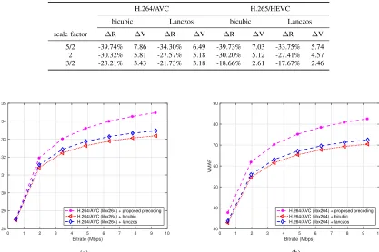
BD-rate [14] gains with respect to PSNR and VMAF are shown in Table II and Table III, respectively. Our precoding is shown to consistently outperform bicubic and Lanczos downscaling for all modes. For PSNR, its BD-rate gains ranged from 8% to 25%, while, for VMAF, rate reduction of 18%-40% is obtained. Indicative rate-distortion curves with

respect to PSNR and VMAF for s = 5/2 factor are shown

TABLE II

BD-RATE(∆R)ANDBD-PSNR (∆P)RESULTS FOR REPRESENTATIVE DOWNSCALING FACTORS.

H.264/AVC H.265/HEVC

bicubic Lanczos bicubic Lanczos

scale factor ∆R ∆P ∆R ∆P ∆R ∆P ∆R ∆P

5/2 -24.70% 0.61dB -19.21% 0.45dB -25.17% 0.55dB -18.84% 0.39dB 2 -18.85% 0.56dB -14.71% 0.42dB -19.25% 0.52dB -14.46% 0.37dB 3/2 -17.11% 0.45dB -11.75% 0.31dB -13.18% 0.32dB -8.26% 0.20dB

TABLE III

BD-RATE(∆R)ANDBD-VMAF (∆V)FOR REPRESENTATIVE DOWNSCALING FACTORS.

H.264/AVC H.265/HEVC

bicubic Lanczos bicubic Lanczos

scale factor ∆R ∆V ∆R ∆V ∆R ∆V ∆R ∆V

5/2 -39.74% 7.86 -34.30% 6.49 -39.73% 7.03 -33.75% 5.74 2 -30.32% 5.81 -27.57% 5.18 -30.20% 5.12 -27.41% 4.57 3/2 -23.21% 3.43 -21.73% 3.18 -18.66% 2.61 -17.67% 2.46

0 1 2 3 4 5 6 7 8 9 10 Bitrate (Mbps)

28 29 30 31 32 33 34 35

Y- PSNR (dB)

H.264/AVC (libx264) + proposed precoding H.264/AVC (libx264) + bicubic H.264/AVC (libx264) + lanczos

(a)

0 1 2 3 4 5 6 7 8 9 10

Bitrate (Mbps) 30

40 50 60 70 80 90

VMAF

H.264/AVC (libx264) + proposed precoding H.264/AVC (libx264) + bicubic H.264/AVC (libx264) + lanczos

(b)

Fig. 6. Rate-distortion curves in terms of (a) PSNR and (b) VMAF for FHD content encoded with H.264/AVC and scale factors= 5/2.

TABLE IV

BD-RATE(∆R)ANDBD-PSNR (∆P)FORFHDCONTENT.

AVC + iSIZE HEVC + iSIZE VP9 + iSIZE

∆R ∆P ∆R ∆P ∆R ∆P

AVC -14.18% 0.70dB - - -

-HEVC - - -8.46% 0.26dB -

-VP9 - - - - -28.95% 1.03dB

AWS -19.50% 0.81dB - - -25.50% 0.74dB

are shown in Fig. 7 and Fig. 8. The improvement in visual fidelity demonstrated in the figures is also captured by the (ap-prox.) 10-point average VMAF difference shown at the 5Mbps point of Fig. 6b. Several of the FHD and UHD video sequences encoded with the proposed precoding and H.264/AVC (and the corresponding H.264/AVC encoded results) are also available for visual inspection at www.isize.co/portfolio/demo. They can be played with any DASH player, since our proposal does not

TABLE V

BD-RATE(∆R)ANDBD-VMAF (∆V)FORFHDCONTENT.

AVC + iSIZE HEVC + iSIZE VP9 + iSIZE

∆R ∆V ∆R ∆V ∆R ∆V

AVC -28.07% 8.35 - - -

-HEVC - - -15.60% 2.91 -

-VP9 - - - - -24.13% 4.61

AWS -43.28% 11.94 - - -30.34% 4.92

require any change at the streaming or client side.

C. Evaluation of Adaptive Precoding for Video-on-Demand Encoding

appro-TABLE VI

BD-RATE(∆R)ANDBD-PSNR (∆P)FORUHDCONTENT.

AVC + iSIZE HEVC + iSIZE VP9 + iSIZE

∆R ∆P ∆R ∆P ∆R ∆P

AVC -53.77% 4.17dB - - -

-HEVC - - -16.63% 0.50dB -

-VP9 - - - - -44.73% 1.57dB

AWS -45.79% 3.38dB - - -39.20% 1.25dB

TABLE VII

BD-RATE(∆R)ANDBD-VMAF (∆V)FORUHDCONTENT.

AVC + iSIZE HEVC + iSIZE VP9 + iSIZE

∆R ∆V ∆R ∆V ∆R ∆V

AVC -46.93% 14.98 - - -

-HEVC - - -21.19% 3.76 -

-VP9 - - - - -30.13% 4.10

AWS -73.13% 31.98 - - -62.61% 13.42

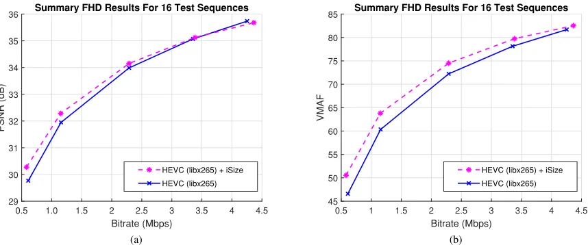
priate for highly-optimized video-on-demand (VOD) encoding systems that are widely deployed today for video delivery. Our evaluation focuses on average bitrate-PSNR and birate-VMAF curves for our test FHD and UHD sequences and we present the results for: H.264/AVC in Fig. 9 and Fig. 10; H.265/HEVC in Fig. 11 and Fig. 12; and VP9 in Fig. 13 and Fig. 14. The corresponding BD-rate gains of our approach in conjunction with each of these encoders vs. the corresponding encoder implementations are presented in Tables IV-VII. For the proposed precoding method, we use footprinting with speed up factor 5, i.e., only every 5th frame is processed during the selection of the best precoding mode, and the same encoding configuration is used as for the corresponding baseline encoder.

Regarding H.264/AVC and H.265/HEVC, we use the high-optimized “slower” preset and VBV encoding for

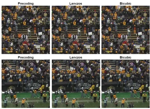
Fig. 7. Two segments of frame 25 of thecrowd runFHD sequence encoded at 5000Kbps with the settings corresponding to Fig. 6. The precoded stream preserves the lettering and overall shapes significantly better than Lanczos and bicubic downscaling. Best viewed under magnification.

Fig. 8. Two segments of frame 77 ofrush field cutsFHD sequence encoded at 5000Kbps with the settings of Fig. 6. The precoded stream preserves the ge-ometric structures significantly better than Lanczos and bicubic downscaling. Best viewed under magnification.

libx264/libx265, with GOP=90, and the widely-used crf=23 configuration for VBV (see footnote 4 for further details). For our approach, we employed (per codec) the precoding modes and crf values shown in Table I. To illustrate that our gains are achieved over a commercially competitive VOD encoding setup, for H.264/AVC we also include results

with the high-performing AWS MediaConvert encoder5 _using

the MULTI PASS HQ H.264/AVC profile and its recently-announced high-performance QVBR mode with the default value of quality level 7. The results of Tables IV-VII show that, against the H.264/AVC libx264 implementation, the av-erage rate saving of our approach for both FHD and UHD resolution under both metrics (PSNR and VMAF) is 36%; the corresponding saving of our approach against H.264/AVC AWS MediaConvert is 45%. For H.265/HEVC libx265, the average saving of our approach is 15%.

Regarding VP9, we employed constant quality encoding with min-max rate (see more details at [48]), GOP=90 frames, maxrate=1.45×minrate, speed=1 for lower-resolution encod-ing (see Table I) and speed=2 for the full-resolution encodencod-ing anchor, since we only utilize downscaled versions with 6% to 64% of the video pixels of the original resolution. Additional bitrate reduction may be achievable by utilizing VBV encoding in libvpx-vp9, but we opted not to use VBV encoding to make our comparison balanced with the VP9 implementation provided by the AWS Elastic Transcoder, which was used as our external benchmark for VP9. The settings of the Elastic Transcoder jobs were based on the built-in presets6_{, which}

we customized to match the desired output video codec, resolution, bitrate, and GOP size, and we set the framerate

5_{AWS tools do not support H.265/HEVC, so no corresponding benchmark}

is presented for that encoder from implementations external to FFmpeg. However, libx265 is well recognized as a state-of-the-art implementation and is frequently used in encoding benchmarks [47].

6

according to the input video framerate. Such customization is necessary because the built-in presets do not follow the input video parameters and they serve mainly as boilerplates. The results of Tables IV-VII show that, against the VP9 libvpx-vp9 implementation, the average rate saving of our approach for both FHD and UHD resolution under both metrics (PSNR and VMAF) is 32%; the corresponding saving of our approach against VP9 AWS Elastic Transcoder, the corresponding saving is 39%.

D. Runtime Analysis for Cloud-based VOD Encoding

Since VOD encoding configurations are typically deployed over a cloud implementation, it is of interest to benchmark the complexity of encoding with our deep video precoding modes versus the corresponding plain encoder. Table VIII presents benchmarks for typical precoding scales on an AWS t2.2xlarge instance with each precoding and encoding running in two threads on two of the Intel Xeon 3.3GHz CPUs. The results correspond to the average processing of each GOP (comprising 90 frames and excluding I/O). By comparing the standard encoding time per video coding standard (scale 1) with our precoding and encoding time for the remaining scales, we see that, as scale increases, the encoding time reduces by up to a factor of five, while precoding time remains quasi-constant. The rate savings versus downscaling by these factors using bicubic and Lanczos filters are shown in Table II and Table III (for FHD content). These results indicate that, especially for the case of complex encoding standards like H.265/HEVC and VP9 that require long encoding times for high-quality VOD streaming systems, the combination of precoding with the appropriate ratio may allow for a more efficient realization on a cloud platform with substantial reduction in rate (or improvement in quality) than using linear filters. In this con-text, precoding effectively acts as a data-driven pre-encoding compaction mechanism in the pixel domain, which allows for accelerated encoding, with the client linearly upscaling to the full resolution and producing high quality video.

VI. CONCLUSION

We propose the concept of deep video precoding based on convolutional neural networks, with the current focus being on downscaling-based compaction under DASH/HLS adaptation. A key aspect of our approach is that it remains backward compatible to existing systems and does not require any change for the streaming, decoder, and display components of a VOD solution. Given that our approach does not alter the encoding process, it offers an additional optimization dimension going beyond content-adaptive encoding and codec parameter optimization. Indeed, experiments show that it brings benefits on top of such well-known optimizations: under high-performing two-pass and VBR-based FHD and UHD video encoding, our precoding offers 15%-45% bitrate saving versus leading AVC/H.264, HEVC and VP9 encoders. The compaction features of our solution ensure that, not only bitrate is saved, but also that video encoding complexity reduction can be achieved, especially for HEVC and VP9 VOD encoding. Future work may consider how to extend the notion

of precoding beyond DASH/HLS systems by learning to adaptively preprocess video inputs such that they are optimally recovered by current decoders under specified bitrate ranges of interest.

REFERENCES

[1] I. Sodagar, “The MPEG-DASH standard for multimedia streaming over the internet,”IEEE multimedia, vol. 18, no. 4, pp. 62–67, 2011. [2] D. Weinberger, “Choosing the right video bitrate for streaming HLS

and DASH,” Feb 2015. [Online]. Available: https://bitmovin.com/ video-bitrate-streaming-hls-dash/

[3] I. Katsavounidis, “Dynamic optimizer: A perceptual video encoding optimization framework,”The Netflix Tech Blog, 2018.

[4] M. Haris, G. Shakhnarovich, and N. Ukita, “Deep back-projection networks for super-resolution,” inProc. of the IEEE Conf. on Computer Vision and Pattern Recognition (CVPR), 2018, pp. 1664–1673. [5] B. Lim, S. Son, H. Kim, S. Nah, and K. M. Lee, “Enhanced deep residual

networks for single image super-resolution,” inProc. of the IEEE Conf. on Computer Vision and Pattern Recognition Workshops (CVPRW), July 2017, pp. 1132–1140.

[6] D. Sculley, G. Holt, D. Golovin, E. Davydov, T. Phillips, D. Ebner, V. Chaudhary, M. Young, J.-F. Crespo, and D. Dennison, “Hidden technical debt in machine learning systems,” in Advances in neural information processing systems, 2015, pp. 2503–2511.

[7] A. Wiesel, Y. C. Eldar, and S. Shamai, “Linear precoding via conic opti-mization for fixed MIMO receivers,”IEEE Trans. on Signal Processing, vol. 54, no. 1, pp. 161–176, Jan 2006.

[8] Y. Tsaig, M. Elad, P. Milanfar, and G. H. Golub, “Variable projection for near-optimal filtering in low bit-rate block coders,”IEEE Transactions on Circuits and Systems for Video Technology, vol. 15, no. 1, pp. 154– 160, 2005.

[9] G. Georgis, G. Lentaris, and D. Reisis, “Reduced complexity superreso-lution for low-bitrate video compression,”IEEE Trans. on Circuits and Systems for Video Technology, vol. 26, no. 2, pp. 332–345, 2016. [10] J. Kopf, A. Shamir, and P. Peers, “Content-adaptive image downscaling,”

ACM Trans. on Graphics (TOG), vol. 32, no. 6, p. 173, 2013. [11] A. C. ¨Oztireli and M. Gross, “Perceptually based downscaling of

images,”ACM Trans. on Graphics (TOG), vol. 34, no. 4, p. 77, 2015. [12] C. G. Bampis, Z. Li, I. Katsavounidis, T.-Y. Huang, C. Ekanadham,

and A. C. Bovik, “Towards perceptually optimized end-to-end adaptive video streaming,”arXiv preprint arXiv:1808.03898, 2018.

[13] Z. Li, A. Aaron, I. Katsavounidis, A. Moorthy, and M. Manohara, “Toward a practical perceptual video quality metric,”The Netflix Tech Blog, vol. 6, 2016.

[14] G. Bjontegaard, “Calculation of average psnr differences between rd-curves,”VCEG-M33, 2001.

[15] J. Kim, J. Kwon Lee, and K. Mu Lee, “Accurate image super-resolution using very deep convolutional networks,” in Proc. of the IEEE Conf. on Computer Vision and Pattern Recognition (CVPR), 2016, pp. 1646– 1654.

[16] B. Lim, S. Son, H. Kim, S. Nah, and K. Mu Lee, “Enhanced deep resid-ual networks for single image super-resolution,” inProc. of the IEEE Conference on Computer Vision and Pattern Recognition Workshops, 2017, pp. 136–144.

[17] C. Dong, C. C. Loy, and X. Tang, “Accelerating the super-resolution convolutional neural network,” inProc. of the European Conference on Computer Vision (ECCV). Springer, 2016, pp. 391–407.

[18] J. Kim, J. Kwon Lee, and K. Mu Lee, “Deeply-recursive convolutional network for image super-resolution,” inProc. of the IEEE Conference on Computer Vision and Pattern Recognition (CVPR), 2016, pp. 1637– 1645.

[19] M. Afonso, F. Zhang, and D. R. Bull, “Video compression based on spatio-temporal resolution adaptation,” IEEE Trans. on Circuits and Systems for Video Technology, vol. 29, no. 1, pp. 275–280, 2019. [20] Y. Li, D. Liu, H. Li, L. Li, F. Wu, H. Zhang, and H. Yang, “Convolutional

neural network-based block up-sampling for intra frame coding,”IEEE Trans. on Circuits and Systems for Video Technology, vol. 28, no. 9, pp. 2316–2330, Sep. 2018.

[21] J. Lin, D. Liu, H. Yang, H. Li, and F. Wu, “Convolutional neural network-based block up-sampling for HEVC,”IEEE Trans. on Circuits and Systems for Video Technology, 2018.

0 1 2 3 4 5 6 7

Bitrate (Mb s)

26 28 30 32 34 36

P

S

N

R

(d

B

)

Summary FHD Results For 16 Test Sequences

AVC/H.264 (libx264) + iSize AVC/H.264 (libx264) AWS MediaConvert QVBR

(a)

0 1 2 3 4 5 6 7

Bitrate (Mb s)

20 30 40 50 60 70 80 90

V

M

A

F

Summary FHD Results For 16 Test Sequences

AVC/H.264 (libx264) + iSize AVC/H.264 (libx264) AWS MediaConvert QVBR

(b)

Fig. 9. Performance comparison of H.264/AVC encoding with proposed adaptive precoding versus standalone H.264/AVC encoding and AWS MediaConvert H.264/AVC encoder (QVBR mode) on FHD content: (a) PSNR and (b) VMAF.

0 2 4 6 8 10 12 14

Bitrate (Mb s)

25 27 29 31 33 35 37 39

P

S

N

R

(d

B

)

Summary UHD Results For 14 Test Sequences

AVC/H.264 (libx264) + iSize AVC/H.264 (libx264) AWS MediaConvert QVBR

(a)

0 2 4 6 8 10 12 14

Bitrate (Mb s)

10 20 30 40 50 60 70 80 90

V

M

A

F

Summary UHD Results For 14 Test Sequences

AVC/H.264 (libx264) + iSize AVC/H.264 (libx264) AWS MediaConvert QVBR

(b)

Fig. 10. Performance comparison of H.264/AVC encoding with proposed adaptive precoding versus standalone H.264/AVC encoding and AWS MediaConvert H.264/AVC encoder (QVBR mode) on UHD content: (a) PSNR and (b) VMAF.

0.5 1.0 1.5 2 2.5 3 3.5 4 4.5

Bitrate (Mb s)

29 30 31 32 33 34 35 36

P

S

N

R

(d

B

)

Summary FHD Results For 16 Test Sequences

HEVC (libx265) + iSize HEVC (libx265)

(a)

0.5 1 1.5 2 2.5 3 3.5 4 4.5

Bitrate (Mb s)

45 50 55 60 65 70 75 80 85

V

M

A

F

Summary FHD Results For 16 Test Sequences

HEVC (libx265) + iSize HEVC (libx265)

(b)

0 2 4 6 8 10 12

Bitrate (Mb s)

33 34 35 36 37 38 39 40 41

P

S

N

R

(d

B

)

Summary UHD Results For 14 Test Sequences

HEVC (libx265) + iSize HEVC (libx265)

(a)

0 2 4 6 8 10 12

Bitrate (Mb s)

60 65 70 75 80 85 90 95

V

M

A

F

Summary UHD Results For 14 Test Sequences

HEVC (libx265) + iSize HEVC (libx265)

(b)

Fig. 12. Performance comparison of H.265/HEVC encoding with proposed adaptive precoding versus standalone H.265/HEVC encoding on UHD content: (a) PSNR and (b) VMAF.

0 1 2 3 4 5 6 7 8

Bitrate (Mb s)

30 31 32 33 34 35 36

P

S

N

R

(d

B

)

Summary FHD Results For 16 Test Sequences

VP9 (libvpx-vp9) + iSize VP9 (libvpx-vp9) AWS Elastic Transcoder

(a)

0 1 2 3 4 5 6 7 8

Bitrate (Mb s)

45 50 55 60 65 70 75 80 85

V

M

A

F

Summary FHD Results For 16 Test Sequences

VP9 (libvpx-vp9) + iSize VP9 (libvpx-vp9) AWS Elastic Transcoder

(b)

Fig. 13. Performance comparison of VP9 encoding with proposed adaptive precoding versus standalone VP9 encoding and AWS Elastic Transcoder VP9 encoder on FHD content: (a) PSNR and (b) VMAF

0 5 10 15 20

Bitrate (Mb s)

32 33 34 35 36 37 38 39 40

P

S

N

R

(d

B

)

Summary UHD Results For 14 Test Sequences

VP9 (libvpx-vp9) + iSize VP9 (libvpx-vp9) AWS Elastic Transcoder

(a)

0 5 10 15 20

Bitrate (Mb s)

40 50 60 70 80 90 100

V

M

A

F

Summary UHD Results For 14 Test Sequences

VP9 (libvpx-vp9) + iSize VP9 (libvpx-vp9) AWS Elastic Transcoder

(b)

TABLE VIII

AVERAGE RUNTIME(MSEC PERGOPONCPU)FOR REPRESENTATIVE DOWNSCALING FACTORS AND MULTIPLE ENCODING BITRATES.

Precoding AVC HEVC VP9

s FHD UHD FHD UHD FHD UHD FHD UHD

1 0 0 1451 4928 11002 54016 3072 594400

3/2 671 4067 745 1982 7634 32565 2107 318445

2 775 4468 529 1854 7476 31786 1763 221522

5/2 703 4408 358 1008 6292 14692 1015 156259

[23] D. Liu, Y. Li, J. Lin, H. Li, and F. Wu, “Deep learning-based video coding: A review and a case study,”arXiv preprint arXiv:1904.12462, 2018.

[24] L. Theis, W. Shi, A. Cunnigham, and F. Husz´ar, “Lossy image com-pression with compressive autoencoders,” inProc. of the Int. Conf. on Learning Representations (ICLR), 2017.

[25] O. Rippel and L. Bourdev, “Real-time adaptive image compression,” in Proc. Int. Conf. on Machine Learning (ICML), vol. 70, Aug. 2017, pp. 2922–2930.

[26] A. Shocher, N. Cohen, and M. Irani, ““zero-shot” super-resolution using deep internal learning,” inProc. of the IEEE Conference on Computer Vision and Pattern Recognition, 2018, pp. 3118–3126.

[27] N. Weber, M. Waechter, S. C. Amend, S. Guthe, and M. Goesele, “Rapid, detail-preserving image downscaling,”ACM Trans. on Graphics (TOG), vol. 35, no. 6, p. 205, 2016.

[28] X. Hou, J. Duan, and G. Qiu, “Deep feature consistent deep image transformations: Downscaling, decolorization and HDR tone mapping,” arXiv preprint arXiv:1707.09482, 2017.

[29] H. Kim, M. Choi, B. Lim, and K. Mu Lee, “Task-aware image downscaling,” inProc. of the European Conference on Computer Vision (ECCV), 2018, pp. 399–414.

[30] F. Jiang, W. Tao, S. Liu, J. Ren, X. Guo, and D. Zhao, “An end-to-end compression framework based on convolutional neural networks,”IEEE Transactions on Circuits and Systems for Video Technology, vol. 28, no. 10, pp. 3007–3018, Oct 2018.

[31] M. Afonso, F. Zhang, and D. R. Bull, “Video compression based on spatio-temporal resolution adaptation,”IEEE Transactions on Circuits and Systems for Video Technology, vol. 29, no. 1, pp. 275–280, 2018. [32] O. Rippel, S. Nair, C. Lew, S. Branson, A. G. Anderson, and L. Bourdev,

“Learned video compression,”arXiv preprint arXiv:1811.06981, 2018. [33] A. Asan, I.-H. Mkwawa, L. Sun, W. Robitza, and A. C. Begen,

“Optimum encoding approaches on video resolution changes: A com-parative study,” in2018 25th IEEE International Conference on Image Processing (ICIP). IEEE, 2018, pp. 1003–1007.

[34] C. Dong, C. C. Loy, K. He, and X. Tang, “Image super-resolution using deep convolutional networks,”IEEE Trans. on Pattern Analysis and Machine Intelligence, vol. 38, no. 2, pp. 295–307, 2016. [35] W.-S. Lai, J.-B. Huang, N. Ahuja, and M.-H. Yang, “Deep Laplacian

pyramid networks for fast and accurate super-resolution,” in Proc. of the IEEE Conf. on Computer Vision and Pattern Recognition (CVPR), 2017, pp. 624–632.

[36] Y. Tai, J. Yang, and X. Liu, “Image super-resolution via deep recursive residual network,” inProc. of the IEEE Conference on Computer Vision and Pattern Recognition (CVPR), 2017, pp. 3147–3155.

[37] Y. Tai, J. Yang, X. Liu, and C. Xu, “Memnet: A persistent memory network for image restoration,” in Proc. of the IEEE Int. Conf. on Computer Vision (ICCV), 2017, pp. 4539–4547.

[38] K. He, X. Zhang, S. Ren, and J. Sun, “Identity mappings in deep residual networks,” inProc. of the European Conf. on Computer Vision (ECCV). Springer, 2016, pp. 630–645.

[39] ——, “Delving deep into rectifiers: Surpassing human-level performance on imagenet classification,” inProc. of the IEEE Int. Conf. on Computer Vision (ICCV), ser. ICCV ’15. Washington, DC, USA: IEEE Computer Society, 2015, pp. 1026–1034.

[40] ——, “Deep residual learning for image recognition,” inProc. of the IEEE Conf. on Computer Vision and Pattern Recognition (CVPR), 2016, pp. 770–778.

[41] X. Glorot and Y. Bengio, “Understanding the difficulty of training deep feedforward neural networks,” inProc. of the13th Int. Conf. on Artificial Intelligence and Statistics, 2010, pp. 249–256.

[42] E. Agustsson and R. Timofte, “NTIRE 2017 challenge on single image super-resolution: Dataset and study,” in Proc. of the IEEE Conf. on

Computer Vision and Pattern Recognition Workshops, 2017, pp. 126– 135.

[43] S. Ma, Wen Gao, and Yan Lu, “Rate-distortion analysis for H.264/AVC video coding and its application to rate control,”IEEE Trans. on Circuits and Systems for Video Technology, vol. 15, no. 12, pp. 1533–1544, Dec 2005.

[44] A. Ortega and K. Ramchandran, “Rate-distortion methods for image and video compression,”IEEE Signal Processing Magazine, vol. 15, no. 6, pp. 23–50, Nov 1998.

[45] “FFmpeg,” https://trac.ffmpeg.org/wiki/Encode/H.264#twopass. [46] “FFmpeg,” https://trac.ffmpeg.org/wiki/Encode/H.264#

AdditionalInformationTips.

[47] J. D. Cock, A. Mavlankar, A. Moorthy, and A. Aaron, “A large-scale video codec comparison of x264, x265 and libvpx for practical VOD applications,” inProc. of SPIE Applications of Digital Image Processing XXXIX, vol. 9971, 2016.