Artificial Algorithms Comparative Study

International Research Journal of Engineering and Technology

(IRJET) e-ISSN: 2395-0056

Volume: 06 Issue: 09 | Sep2019 www.irjet.net p-ISSN: 2395-0072

© 2019, IRJET | Impact Factor value: 7.34 | ISO 9001:2008 Certified Journal | Page 847

ARTIFICIAL ALGORITHMS COMPARATIVE STUDY

Kaushik Indranil Patil

1

_{, Simran Sachin Sura}

2

1

_{Nashik District Maratha Vidya Prasarak Samaj's Karmaveer Baburao Thakare College of Engineering, Nashik,}

Maharashtra, India.

2

_{Smt.Kashibai Navale College of Engineering, Vadgaon, Pune, Maharashtra, India.}

---***---Abstract

— This paper showcases a comparative study of

some commonly used Artificial Intelligence algorithms such as Heuristics, A*algorithm, KNN, Linear Regression. In this paper, we illustrated an example of each algorithm describing its solution. Through this paper, the author demonstrates the variety of problems that can be solved by the above mentioned AI algorithms thus giving the reader an idea about which algorithm to apply to which AI problem.

Key Words: Artificial intelligence, Heuristics, A*, KNN, Linear Regression.

1. INTRODUCTION

Conventional computer programming lacks the ability to solve complex problems where the output result varies greatly on a number of inputs Thus, It has become necessary to develop some methods to solve a certain type of problems which can not be efficiently solved by conventional computer programming. As an example, let’s consider a chess-playing program. Theoretically, there are

around _{legal moves possible in a chess game. Now}

it is practically impossible to program a machine to handle each and every of possible moves. Thus, it is necessary to develop a machine which is able to play the game of chess in a way similar to how humans play. Thus came the evolution of Artificial Intelligence algorithms.

There doesn’t exist such an algorithm called “Unified Artificial Intelligence Algorithm”. There are many artificial intelligence algorithms developed but one algorithm for all doesn't exist. Thus it becomes very necessary to be able to recognize which algorithm to be applied to which scenario. In this paper, we have presented five types of AI algorithms namely Heuristics, A* algorithm, Linear Regression, KNN.

Section I: Introduction, introduces the paper topic. Section II: Heuristic Algorithm, discusses the analysis of heuristic algorithm and how water jug problem can be solved using heuristics. Section III: A* algorithm discusses the types of pathfinding algorithms and discusses A* algorithm in-depth with pseudo code. Section IV: Linear Regression discusses the Linear Regression algorithm in detail, Section V: KNN, which introduces to KNN algorithm with some visual examples. Section VI: Concludes the paper.

2. HEURISTICS ALGORITHM

A Heuristic is a technique to solve a problem faster than the classical method such as looping through a number of steps until a solution is reached, or to find an approximate solution when classic methods cannot. Heuristic algorithms can be called a shortcut which improves optimization, completeness, accuracy, precision and speed. At each branching step of the heuristic algorithm, it evaluates the information that is available and makes a decision on which branch is to be followed next. It does so by ranking alternatives. The Heuristic algorithm is often effective but does not guarantee to work in every case.

2.1 Solving the Water Jug Problem

Heuristic solutions rely upon problem-solving methods evolved from practical experience, they are rules of thumb that try to estimate an acceptable, computationally effective solution, as close as possible to the optimal one. However, they do not guarantee that a solution will be obtained at all. They are only believed to work in most situations. There are specific heuristics that are applicable to a particular situation, and general heuristics that are applicable to a large range of problems. Let us consider a heuristic for the generalized water jugs problem: if the rest is lower than the capacity of jug A, the problem has no solution (obvious); if the rest is a multiple of the greatest common divisor of A and B, the problem has no solution (the solution results from combining the differences between A and B; e.g. with A=6 and B=3, it is impossible to obtain a rest equal to 2, because all the differences will be multiples of three); since the solution of this problem is based on the water exchange between the two containers in order to obtain the differences, there are two strategies that lead to the solution for any problem. Let value ‘A’ and value ‘B’ be the quantities of the two jugs, respectively. Let rest be the quantity that is to be obtained in the first jug.

Strategy 1: while (valA != rest) { if (valB != B && valA == 0) FillA(); if (valB == B) EmptyB(); Pour FromAtoB(); }

International Research Journal of Engineering and Technology

(IRJET) e-ISSN: 2395-0056

Volume: 06 Issue: 09 | Sep2019 www.irjet.net p-ISSN: 2395-0072

[image:2.595.53.259.81.244.2]

© 2019, IRJET | Impact Factor value: 7.34 | ISO 9001:2008 Certified Journal | Page 848

Fig - 1: Efficiency of the Heuristic method. X-Axis: Steps to

Solution, Y-Axis: Efficiency.

In this way, building a solution tree is not required and solving is done without additional memory costs. However, since they are heuristic solutions, the adequate strategy should be determined from case to case. For example, if the value of A=6 and value of B=5 and the rest is 2, the first strategy finds the solution in 6 steps, while the latter does in 14 steps. If A=11, B=6 and the rest is 7, the first strategy finds the solution in 24 steps, and the latter is only 8.

3. A* ALGORITHM

A pathfinding algorithm initializes graph search by starting at one vertex and exploring adjacent vertices until the destination vertex is reached, generally with the intent of finding the most optimal route but not necessarily the most efficient. Pathfinding algorithm consists of two phases

1. Finding the path between two given nodes.

2. Finding the most optimal path between the two nodes.

Types of pathfinding algorithm:

1. Exhaustive.

2. Eliminatory.

Let's first look at what Exhaustive algorithms are.

1. Exhaustive pathfinding algorithms

The most primitive pathfinding algorithms are Breadth-first and Depth-Breadth-first. This algorithm finds the path between two nodes by exhausting all the possibilities, starting from a given node. These algorithm run in O(|V| + |E|), or linear time, where V is the number of vertices, and E is the number of Edges between vertices.

Another yet complicated pathfinding algorithm for finding the optimal path is the Bellman-Ford algorithm, which yields the time complexity of O(|V||E|), or quadratic time.

However, it is not necessary to examine all the possible paths to find the optimum one.

2. Eliminatory pathfinding algorithms

The eliminatory algorithms consist of Dijkstra and A* pathfinding algorithms. In this project, A* algorithm is implemented due to the high time cost of Dijkstra and the inability of Dijkstra to evaluate negative edge weights.

3.1 A star algorithm

:

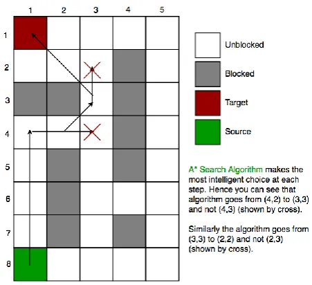
A* is a variant of Dijkstra's algorithm. A* assigns a weight to each open node which is equal to the weight of the edge to that node in addition to the approximate distance between that node and the finish. This approximate distance is found by the heuristic 1 and represents a minimum possible distance between that node and the end. This enables it to eliminate longer paths once an initial path is found. If there exists a path of length x between the start and finish, and the minimum distance between a node and the finish is greater than the distance x, that node does not need to be examined. A* uses this heuristic to improve on the behaviour relative to Dijkstra's algorithm. When the heuristic evaluates to zero, A* is equivalent to Dijkstra's algorithm[12]. As the heuristic estimate increases in magnitude and also gets closer to the true distance, A* continues to find optimal paths and runs faster because it needs to examine fewer nodes than before thus less computation required. A* examines the fewest nodes when the value of the heuristic is exactly the true distance,

Fig - 2. Illustration of A* search algorithm[13].

A* f cost calculation equation:

f(n) = g(n) + h(n) … (1)

Where:

[image:2.595.318.544.453.659.2]

International Research Journal of Engineering and Technology

(IRJET) e-ISSN: 2395-0056

Volume: 06 Issue: 09 | Sep2019 www.irjet.net p-ISSN: 2395-0072

© 2019, IRJET | Impact Factor value: 7.34 | ISO 9001:2008 Certified Journal | Page 849

excluding the unwalkable path.

h is the cost of the present node from the ending point including the unwalkable path.

[image:3.595.330.542.120.245.2]

f is the resultant cost.

Fig Fid - 3: A* pseudo code[11]

Application of A* in real-world scenarios:

1. Calculate the shortest path between two locations

on a map.

2. A* is vastly used in game development wherein it

is required to obtain the shortest path between two points.

3. Parsing Stochastic grammars in Natural Language

Processing.

4. LINEAR REGRESSION

Let's get to know about Linear Regression algorithm with the help of an example first, consider a situation wherein, you are required to arrange random logs of work in ascending order of their weight, but there is a condition: you are not allowed to weigh each log, so you have only one option: to guess the weight of each log just by visual analysis. This is exactly the type of problem which can be solved by linear regression.

The Linear regression algorithm uses the mathematical equation: y = bx + a. This equation describes the line of best fit for the relationship between the dependent variable(y) and the independent variable(x).

Following equation governs the Linear regression algorithm[16]:

Where Eq. 2 gives the y-intercept(a) and Eq. 3 gives the slope of line(b).

Thus Linear Regression is very significant due to the following reasons:

1. It helps understand the strength of the

relationship between the outcome and the predictor variable.

2. Linear Regression can make an adjustment for the

effect of covariance.

3. Through Linear Regression, we can get to know

the risk factor affecting the dependent variable.

4. It also helps in quantifying new cases in our

problem statement.

Regression analysis provides us with three things[14]:

1. Description: Relation between dependent and

independent variables.

2. Estimation: Value of the dependent variable can be

estimated from observed values on the independent variables.

3. Risk factor: Upcoming risk factor can be predicted

beforehand to avoid a critical situation in certain analysis scenarios.

Assumptions for linear regression[15]:

1. Values of the independent variable on the X-axis is

set by the researcher.

2. The value of X-axis does not have any

experimental error.

3. All the values of Y are independent of each other

International Research Journal of Engineering and Technology

(IRJET) e-ISSN: 2395-0056

Volume: 06 Issue: 09 | Sep2019 www.irjet.net p-ISSN: 2395-0072

[image:4.595.44.291.59.209.2]

© 2019, IRJET | Impact Factor value: 7.34 | ISO 9001:2008 Certified Journal | Page 850

Fig - 4. A plot of cricket runs vs over, Blue Line depicts the

current score, the yellow line shows expected score.

Applications of Linear Regression algorithm:

1. Data prediction involving one dependent and one

independent variable.

2. Customer Survey analysis.

3. Market Research Studies.

5. KNN ALGORITHM

KNN is one of the most popular. KNN is used for

classification and prediction problems involving

[image:4.595.322.517.86.248.2]

regression. KNN is generally used in a scenario involving multiple data points which need to be classified on the basis of certain aspects. KNN clusters data points based on some similarities they exhibit,

Fig - 5. Pseudo Code for KNN algorithm.

[image:4.595.77.253.454.677.2]

Let’s consider the example below to get a clear idea of the algorithm:

Fig - 6. Example of KNN algorithm.

KNN is used to classify and clusterize input datasets based on certain parameters.

Most commonly used distance functions for calculating distance between input data points are Euclidean and Manhattan [17][18].

=

√∑

… (4)

∑

|

|

… (5)

Where Eq. 4 gives the Euclidean distance and Eq. 5 gives Manhattan distance. While Euclidean distance is most commonly used, the Manhattan method is used for continuous variables.

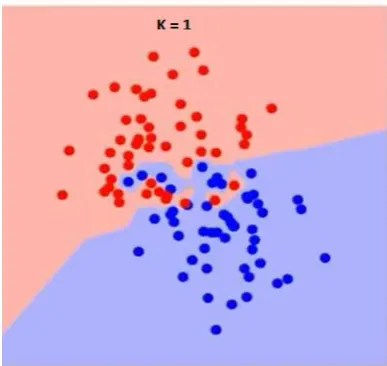
Increasing the K factor makes the algorithm more aggressive. So the classifying boundary between input data points smoothes out. On the other hand, reducing the K factor makes the algorithm more lenient and thus while the classification of data points the reduced K algorithm also considers some conflicting data points also.

Let’s have a look at the figure below showing the effect of the K factor in the KNN algorithm[19].

[image:4.595.334.528.557.740.2]

International Research Journal of Engineering and Technology

(IRJET) e-ISSN: 2395-0056

Volume: 06 Issue: 09 | Sep2019 www.irjet.net p-ISSN: 2395-0072

[image:5.595.65.267.67.282.2]

© 2019, IRJET | Impact Factor value: 7.34 | ISO 9001:2008 Certified Journal | Page 851

Fig - 7. Classification of data points having two classified

regions with K factor kept = 7.

Thus from the above figures: Fig 6 and Fig 7. We can observe that increasing K factor makes the algorithm more aggressive.

Keeping the K factor is up to the engineer, there is a certain trend of value of K and the error rate produced by the algorithm. Following is the graphical representation:

Fig - 8: Graph of Effect of K value on KNN accuracy, K value on the X-Axis, and error rate on the Y-Axis[19].

6. CONCLUSION

In this paper, we have compared various commonly used Artificial Intelligence algorithms with their description, significance, mathematical model as well as their applications. Thus we have successfully showcased the usage of each algorithm in various real-life scenarios. From this paper, one can differentiate between various A algorithms and apply the most suitable algorithm on the given problem.

REFERENCES

[1] Harris R. Creative Problem Solving: A Step by Step Approach, Pyrczak, Los Angeles, 2002.

[2] Boldi P., Santini M., Vigna S. Measuring with Jugs, Theoretical Computer Science, no. 282, pp. 259-270, 2002.

[3] Russell S. J., Norvig P. Artificial Intelligence: A Modern Approach, Prentice Hall, Englewood Cliffs, New.

[4] A Heuristic for Solving the Generalized Water Jugs Problem Bulletin of the Polytechnic Institute of Iasi, tome LI (LV), section Automatic Control and Computer Science.

[5] Vinod Goel, Sketches of thought, MIT Press, 1995, pp.

87 and 88.

[6] Bonnie Averbach and Orin Chein, Problem Solving Through

Recreational Mathematics, Courier Dover Publications,

2000, pp.

156.

[7] H. E. Dudeney, in Strand Magazine vol. 68 (July 1924),

pp. 97 and

214

[8] Pseudo code for Crypt arithmetic problem from https://www.google.com/amp/s/www.geeksforgeeks.org /solving-cryptarithmetic-puzzles-backtracking-8/amp/

[9] Desiani, Anita and Arhami, Muhammad. 2006. Konsep Kecerdasan Buatan. Yogyakarta, Indonesia: C.V Andi Offset.

[10] Ms. Avinash Kaur, Ms. Purva Sharma, Ms.Apurva Verma, International Journal of Scientific and Research Publications, Volume 4, Issue 3, March 2014.

[11] A star algorithm through

https://www.youtube.com/watch?v=-L-WgKMFuhE by

Sebastian Lague.

[12] For detail A* understanding:

http://theory.stanford.edu/~amitp/GameProgramming/H euristic

[13] A* Search Algorithm Blog, GeeksforGeeks.org

[14] Astrid Schneider, Gerhard Hommel, and Maria Blettner; Linear Regression Analysis Part 14 of a Series on Evaluation of Scientific Publications.

[15] Khushbu Kumari, Suniti Yadav; Linear regression analysis study

[image:5.595.49.277.414.573.2]

International Research Journal of Engineering and Technology

(IRJET) e-ISSN: 2395-0056

Volume: 06 Issue: 09 | Sep2019 www.irjet.net p-ISSN: 2395-0072

© 2019, IRJET | Impact Factor value: 7.34 | ISO 9001:2008 Certified Journal | Page 852

[17] Li-Yu Hu, Min-Wei Huang, Shih-Wen Ke, and

Chih-Fong Tsai; The distance function effect on k-nearest neighbor classification for medical datasets.

[18] Punam Mulak, Nitin Talha; Analysis of Distance Measures Using K-Nearest Neighbor Algorithm on KDD Dataset.