A Swarm based Algorithm for Solving Economic Load Dispatch Problem

A Swarm-based Algorithm for Solving Economic Load

Dispatch Problem

Esraa Salem Al-Manaseer

Al-Balqa Applied University Al-Salt, Jordan

Hind Mousa Al-hamadeen

Al-Salt, Jordan

Abdelaziz I. Hammouri

Applied University Al-Salt, Jordan

ABSTRACT

Economic Load Dispatch problem (ELD) is considered a NP-hard combinatorial optimization problem. The function of (ELD) determines low price process regarding a power system through dispatching the power generation sources in order according to supply the load demand. In this paper, one of the most known electrical problems has been displayed by the (ELD). Various methods have been used to make the ELD solutions better, most well-known employing meta-heuristic algorithms. The aim of paper is to find the optimal or near-optimal ELD fuel cost (fuel cost with the minimum cost) by involving a newly created meta-heuristic algorithm, mainly Salp Swarm Algorithm (SSA). Using four test systems generating datasets, the swarm intelligence (SI) has contributed in creating the notion of SSA to get the required value of the present approach. Moreover, it will be measured and contrasted with other similar types or with those of the same significant style that are available in the literature. Accordingly, the results make it clear that the SSA is able to represent the ELD problem and it able to obtain acceptable solutions.

Keywords

Economic Load Dispatch, Salp Swarm-Based Algorithm, swarm intelligence, optimization, meta-heuristic, population based algorithm.

1.

INTRODUCTION

Economic Load Dispatch problem (ELD) is considered a NP-hard combinatorial optimization problem. The function of (ELD) determines low price process regarding a power system through dispatching the power generation sources in order to supply the load demand. In this research, one of the most known electrical problems has been displayed by the (ELD). Various methods have been used to make the ELD solutions better, most well known employing meta-heuristic algorithms.

The major aim in this paper is to attempt solving the problem of Economic Load Dispatch (ELD) by using one of the newest meta-heuristics algorithms (Salp Swarm Algorithm), and making some amendments to this Algorithm.

2.

ELD PROBLEM FORMULATION

The Economic Load Dispatch (ELD) is a vital operation in a fashionable power grid like unit commitment, Load prediction, At the Market Transfer Capability (ATC) calculations, Security Analysis, and planning of fuel purchase etc. To approach the problem of ELD, different numerical optimization techniques have been employed [1]. In classical way, ELD problem is overcome by depending mathematical programs that built upon optimization methods and mechanisms such as: lambda iteration, gradient method [2], [3]. Complex restricted ELD is tackled by intelligent methods.

These methods include various algorithms: genetic algorithm (GA) [4], Evolutionary Programming (EP) [5], Tabu Search [6], and Particle Swarm Optimization (PSO) [3, 7] etc. For calculation simplicity, current ways are used the second order fuel value functions that involve approximation and constraints area unit which is handled singly, though generally valve-point effects area unit thought-about.

ELD is known as a process at the aim of sharing the total load of power system among the several power generation stations in order to achieve highest economy of operation. However, it is possible solving the problem of the ELD (nonlinear optimization problem) by producing an ideal amount of power from the fossil fuel. This can be achieved by downsizing the fuel cost as well as satisfying all system restrictions of power system. It is necessary noting that, the careful and smart scheduling of the generating units will decrease the cost of operating cost significantly besides assuring higher reliability and security of power system [8, 9].

The “classical economic dispatch” downside to find the best combination of power generation that minimizes the whole fuel value, whereas satisfying the whole needed demand are often formulated in the following equation: [6, 10] :

+ ) (1) Where:

 Fi (Pi) denotes Total Fuel Cost ($/h).

 ai, bi, ci denotes Fuel cost parameters of generator i.

 Pi denotes the generated power of generator i (MW Mega Watt).

 n denotes the quantity of generators.  Constraints

The optimization drawback is confined by two kind’s constraints

1. Equality constraints

The volume power generated should stay the equal as like the total request in addition to the total transmission losses.

(2)

Where:

2. inequality constraints

It is necessary that power generation of each generator takes place between extreme and lowest values of power generation, which can be defined as the following:

Pi(min) ≤Pi≤Pi(max) (3)

Where: Pi(min) is the minimum generation of power. And Pi(max) is the maximum generation of power.

In ELD with ‘‘valve point loadings’’, where objective function F is showed using complicated equation, as shown in the eq. (1.4):

F = min ( )

=min( )

(4)

Where: ai, bi, ci, ei, fi are the cost coefficients of unit i.

Hence, the aim of the ELD problem is decreasing the total fuel cost at the thermal power plants and respond with the requirement of a power system while satisfying equality and a set of inequality constraints [11].

We suggested and introduced a newly greated algorithm for solving this problem, it is called “Salp Swarm algorithm (SSA)” which helps to obtain:

1. An improved solution with low fuel cost.

2. Improve the initial random solutions.

3.

META-HEURISTIC ALGORITHM

FOR ELD

The researcher interested in meta-heuristic techniques, especially in the last years, in many different areas that focus on many different issues, such as: scheduling problems [12-16], data classification [17], time series [18, 19], data clustering [20, 21], and global optimization [22]. Because of these methods, have multiple capabilities, the researchers concerned in depending them in developing solutions for the aim of resolving ELD. Based on the obtained results, it was found that applying such these methods on ELD achieved high efficiency and provided robust solutions.

We provide a number of algorithms, which have dealt with Economic Load Dispatch.

 Particle Swarm Optimization:  Genetic Algorithm

 Harmony Search Algorithm  Grey Wolf Algorithm  Krill Herd Algorithm  Salp Swarm Algorithm  Differential Evolution  Cuckoo Search

 Teaching Learning Based Optimization  Social Spider Algorithm

 Backtracking Search Algorithm  Chaotic Bat Algorithm

3.1

Work Mechanism of Salp Swarm

Algorithm

Salp Swarm Algorithm (SSA) [23] is a novel optimization algorithm for solving optimization problem. The main revelation of SSA is the swarming behaviour of salps when navigating and foraging in oceans.

Salps are also pelagic tunicates together with a complicated life cycle that alternates sexual (solitary) and asexual (aggregate) generations. Huge swarms of salps periodically improve with remarkable rapidity and contain enormous numbers regarding animals. These swarms are well known to many oceanographers as nuisances that clog plankton nets, however, Salps also play an essential energetic role great areas of the ocean. [24].

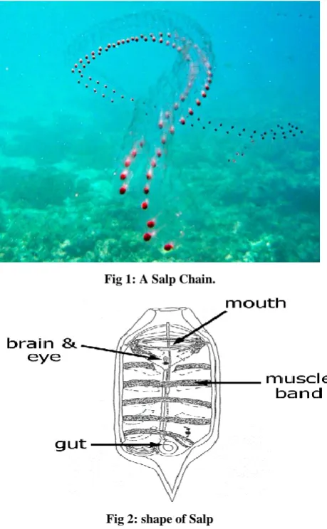
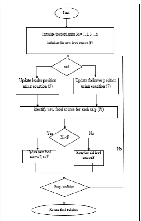
Biological researches of this creature are still in the early milestones, mainly because their living habitats are extremely inaccessible, and it is fairly difficult to sustain them in a laboratory environment. One of the most interesting behavioral characteristics of salps is their highly sophisticated swarming behavior. In deep oceans, salps often form a swarm called salp chain. This chain is illustrated in Figure 1, and the shape of salp is shown in Figure (2) below.

Fig 1: A Salp Chain.

Fig 2: shape of Salp

followers depend on other salps in the chain. A design concept of salp chain is established in (Figure 3). [23, 25, 26].

Fig 3: Illustration of a Salp Chain.

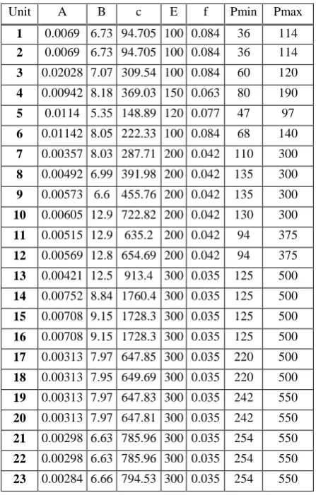
Figure 4 and 5 shows the flowchart and the pseudo-code of the original SSA, respectively.

Fig 4: Flowchart of SSA.

Fig 5: Pseudo code of the SSA algorithm

3.2

Improvement Phase for the SSA

algorithm

Improve the initial solution by update the position of the leader as shown in the following equation:

= – – –

(5)

Where ( ) shows the position of the salp heading a chain (the leader)in a given (j-th) dimension. ( ) is the position of a food source in the (j-th) dimension, while ( ) indicates the upper bound of the(j-th) dimension, ( ) represents the lower bound of the (j-th) dimension. (C1), (C2), and (C3) are just

random numbers.

The above equation shows that the leader only modifies its current position depending on the food source location. The coefficient (C1), is the most significant parameter in the SSA,

since it balances both the exploration, and exploitation as defined in following equation [23]:

C1=2

(6)

Where (l) is the current iteration and (L) is the maximum number of iterations.

The parameters (C2) and (C3) are random numbers uniformly

generated in the interval of [0,1]. In fact, they dictate the step size and whether the next position in the (j-th) dimension should be leaning towards positive or negative infinity.

The below equation (Newton’s law of motion) is applied to modify the following salps positions [23].

Xji= at2 + v0t (7)

where (i≥2), (Xj-i) shows the position of the(i-th) follower salp

in the (j-th) dimension, (t) stands for time, and (v0) is the

initial speed, (a) is calculated as shown in the following equation:

a=vfinal/v0 (8)

where v = (x-x0)/t Because the time used to attain

between iterations is equal to (1), and v0 is assumed to equal zero. Eventually, the following equation can be produced:

Xji= (Xji + Xji-1) (9)

Where (i≥2) and (xji) shows the position of an (i-th) follower salp in a (j-th) dimension.

SSA goes through several steps: firstly, the SSA algorithm initiates several salp at unsystematic positions to approach the global optimum. After that, it computes the each individual salp fitness to locate the fittest salp. Once the fittest salp is determined, its position is assigned to the variable (F), which denotes the food source that a certain salp chain is targeting. In the time being, the coefficient (C1) is changed for each of the dimensions, and the leading and following salps positions are consequently modified. If any of the salps goes astray beyond the search space, it will be located and brought back to be included within the search space margins.

4.

EXPERIMENTAL RESULTS

The SSA performance was assessed in this research through four testing systems (6, 13, 15, 40) generating units.

4.1

Input Parameters

Experiments of the SSA were implemented using Net Beans IDE 8.2 platform on a Windows 10 pro operating system, and a mother board of Intel Core i7 8th generation CPU, and an 8 GB DDRAM. Input parameters in the four testing systems (6 generators, 13 generators, 15 generators, and 40 generators) were incorporated in all of the experiments that were conducted based on the values shown in the below tables (1,.2,.3, and.4) [27, 28].

Table 1: Shows Input Parameters of the First Testing System1 (6 Generators)

Unit A B C Pmin Pmax

1 0.0070 7.0 240 100 500

2 0.0095 10.0 200 50 200

3 0.0090 8.5 220 80 300

4 0.0090 11.0 200 50 150

5 0.0080 10.5 220 50 200

6 0.0095 12.0 190 50 120

Table 2: Shows Input Parameters of the Second Testing System2 (13 Generators)

Unit A B C E f Pmin Pmax

1 0.00028 8.1 550 300 0.035 0 680

2 0.00056 8.1 309 200 0.042 0 360

3 0.00056 8.1 307 200 0.042 0 360

4 0.00324 7.74 240 150 0.063 60 180

5 0.00324 7.74 240 150 0.063 60 180

6 0.00324 7.74 240 150 0.063 60 180

7 0.00324 7.74 240 150 0.063 60 180

8 0.00324 7.74 240 150 0.063 60 180

9 0.00324 7.74 240 150 0.063 60 180

10 0.00284 8.6 126 100 0.084 40 120

11 0.00284 8.6 126 100 0.084 40 120

12 0.00284 8.6 126 100 0.084 55 120

13 0.00284 8.6 126 100 0.084 55 120

Table 3: Shows Input Parameters of the Third Testing System3 (15 Generators)

Unit A B C Pmin Pmax

1 0.000299 10.1 671 150 455

2 0.000183 10.2 574 150 455

3 0.001126 8.8 374 20 130

4 0.001126 8.8 374 20 130

5 0.000205 10.4 461 150 470

6 0.000301 10.1 630 135 460

7 0.000364 9.8 548 135 465

8 0.000338 11.2 227 60 300

9 0.000807 11.2 173 25 162

10 0.001203 10.7 175 25 160

11 0.003586 10.2 186 20 80

12 0.005513 9.9 230 20 80

13 0.000371 13.1 225 25 85

14 0.001929 12.1 309 15 55

15 0.004447 12.4 23 15 55

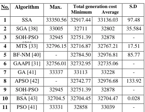
Table 4: Shows Input Parameters of the Fourth Testing System4 (40 Generators)

Unit A B c E f Pmin Pmax

1 0.0069 6.73 94.705 100 0.084 36 114

2 0.0069 6.73 94.705 100 0.084 36 114

3 0.02028 7.07 309.54 100 0.084 60 120

4 0.00942 8.18 369.03 150 0.063 80 190

5 0.0114 5.35 148.89 120 0.077 47 97

6 0.01142 8.05 222.33 100 0.084 68 140

7 0.00357 8.03 287.71 200 0.042 110 300

8 0.00492 6.99 391.98 200 0.042 135 300

9 0.00573 6.6 455.76 200 0.042 135 300

10 0.00605 12.9 722.82 200 0.042 130 300

11 0.00515 12.9 635.2 200 0.042 94 375

12 0.00569 12.8 654.69 200 0.042 94 375

13 0.00421 12.5 913.4 300 0.035 125 500

14 0.00752 8.84 1760.4 300 0.035 125 500

15 0.00708 9.15 1728.3 300 0.035 125 500

16 0.00708 9.15 1728.3 300 0.035 125 500

17 0.00313 7.97 647.85 300 0.035 220 500

18 0.00313 7.95 649.69 300 0.035 220 500

19 0.00313 7.97 647.83 300 0.035 242 550

20 0.00313 7.97 647.81 300 0.035 242 550

21 0.00298 6.63 785.96 300 0.035 254 550

22 0.00298 6.63 785.96 300 0.035 254 550

24 0.00284 6.66 794.53 300 0.035 254 550

25 0.00277 7.1 801.32 300 0.035 254 550

26 0.00277 7.1 801.32 300 0.035 254 550

27 0.52124 3.33 1055.1 120 0.077 10 150

28 0.52124 3.33 1055.1 120 0.077 10 150

29 0.52124 3.33 1055.1 120 0.077 10 150

30 0.0114 5.35 148.89 120 0.077 47 97

31 0.0016 6.43 222.92 150 0.063 60 190

32 0.0016 6.43 222.92 150 0.063 60 190

33 0.0016 6.43 222.92 150 0.063 60 190

34 0.0001 8.95 107.87 200 0.042 90 200

35 0.0001 8.62 116.58 200 0.042 90 200

36 0.0001 8.62 116.58 200 0.042 90 200

37 0.0161 5.88 307.45 80 0.098 25 110

38 0.0161 5.88 307.45 80 0.098 25 110

39 0.0161 5.88 307.45 80 0.098 25 110

40 0.00313 7.97 647.83 300 0.035 242 550

4.2

Comparison with Methods

In this paper there are four different testing systems of different computational complexity levels were carried out to test the SSA algorithm effectiveness. 50 individual trial runs were carried out to determine the performance of SSA . The results of the optimum and mean fuel cost were listed for each of the four testing systems. For the 6 generators problem, the average run time was around (18.82101 seconds), which was the first testing system, and (31.6979 seconds) for the 40generators problem, which was the last testing system. The comparisons are illustrated in tables below.

Table 5: Fuel Cost and Statistical Results for 50Trial Runs of the First Testing System1 (6 Unit Testing System)

No. Algorithm Mean

Fuel Cost ($/hr) Best Fuel Cost ($/hr) Max. Fuel Cost($/hr) Run Time (s) S. D

1 SSA 15470.32 15444.88 15515.83 18.82 17.95

2 NPSOLRS [29]

15454 15450 15452 NA NA

3 DE[30] 15449.62 15449.58 15449.65 3.634 NA

4 GA[31] 15469.21 15451.66 15519.87 NA NA

5 MABC [32] 15449.89 15449.89 15449.89 0.62 0.0

6 GAAPI[31] 15449.81 15449.78 15449.85 NA NA

7 MTS [33] 15451.17 15450.06 15450.06 1.29 0.93

8 SA[33] 15488.98 15461.1 15461.1 50.36 28.37

9 TS[33] 15472.56 15454.89 15454.89 20.55 13.72

10 CBA [27] 15454.76 15450.23 15518.65 0.704 2.97

These results show that SSA is significantly better than other algorithms in the comparison in generating. In terms of standard deviation, the values that were acquired by SSA are much less than most of the methods compared with, which confirms that the SSA algorithm is stable in finding at optimal solutions. Whereas the minimum value of the Mean Fuel Cost is (15,449.81$/hr). In addition, the minimum value of the Max. Fuel Cost is (15,449.6508 $/hr). Moreover, the minimum run time is (0.62s) and the minimum standard deviation is (0.9287). Table 6 shows a testing system that has

just over twice the number of generator, which consists of 13generators with a load demand of 1800 MW. It contains valve point loading, which can introduce a number of local minima, thus creating a multimodal cost curve. The best cost achieved by SSA is (18,751.11 $/hr). It is taken into account that all the generations meet the generation limit constraints.

Table 6: Fuel Cost and Statistical Results for 50Trial Runs of the Second Testing System2 (13 Unit Testing System)

no. Algorithm Mean

Fuel Cost ($/hr) Best Fuel Cost ($/hr) Max. Fuel Cost ($/hr) Run Time (S) S. D

1 SSA 18810.18 18751.11 19019.61 12.48 112.3

2 PSO-SQP [34] 18029.99 17969.93 NA 33.97 NA

3 HCRO-DE [35]

17960.59 17960.38 17961.04 4.91 0.069

4 EP [34] 18127.06 17994.07 NA 157.43 NA

5 CE-SQP [36] 17965.97 17963.85 NA NA NA

6 PSO [34] 18205.78 18030.72 NA 77.37 NA

7 EP-SQP [35] 18106.93 17991.03 NA 121.93 NA

8 CEP [37] 18190.32 18048.21 18404.04 NA NA

9 IFEP [37] 18127.06 17994.07 18267.42 NA NA

10 CGA_MU [36]

- 17975.34 NA NA NA

11 CBA[3] 17965.48 17963.83 17995.22 0.97 6.85

Table 7: Convergence Results for 50Trial Runs of the Third Testing System3 (15 Unit Testing System)

No. Algorithm Max. Total generation cost

Minimum Average S.D

1 SSA 33350.56 32917.44 33136.03 97.48

2 SGA [38] 33005 32711 32802 35.584

3 SOH-PSO [39]

32945 32751.39 32878 -

4 MTS [33] 32796.15 32716.87 32767.21 17.51

5 BF-NM [40] - 32784.50 32976.81 85.77

6 GAAPI [31] 32756.01 32732.95 32735.06 -

7 GA [41] 33337 33113 33228 -

8 APSO [42] - 32742.77 32976.68 133.92

9 SOH-PSO [39]

32945 32751.39 32878 -

10 BSA [43] 32704.5 32704.45 32704.47 0.028

11 PSO [41] 33331 32858 33039 -

This testing system consists of 15 generating units. The data used is obtained from Table 3 and the power demand is 2630 MW. The results achieved by SSA are compared with other methods in Table (7). The results in this table show that the other methods achieved better results in terms of best fuel cost, which make them better than SSA.

superior to the results achieved by SSA, however, SSA ranked seventh of twenty methods for run time.

Figures (6,7,8, and 9) indicate the graphs on the convergence curve of the best obtained solutions in each iteration for the SSA algorithm for a normal run. As shown in these figure the SSA have a fast convergence, where it can improve the solution quickly at the beginning of the search process, after that, the SSA entered the stagnant stage, where the solution has been improved slowly. The comparison showed impressive SSA results exceeding the ones generated by other existing methods found in the literature review, especially when the number of generators used was small.

Table 8: Fuel Cost and Statistical Results for 50 Trial Runs of the Fourth Testing System4 (40 Unit Testing

System)

No Algorithm Mean Fuel Cost

Best Fuel Cost

Max Fuel Cost

Run Time

S.D

1 SSA 141542.2 128875.1 155701.6 31.70 6539.4

2 PSO-SQP [24]

122245.2 122094.6 NA NA NA

3 DSD [36] - 121412.5 NA NA NA

4 HCRO-DE [35]

121413.1 121412.5 121415.68 7.64 91

5 NPSO-LRS

[29]

122209.3 121664.4 122981.5 3.93 NA

6 MABC [32]

121431.58 121412.59 121493.19 1.92 18.1

7 DE [30] 121439.89 121412.68 121479.63 31.503 NA

8 CE-SQP [36]

121423.65 121412.88 NA NA NA

9 BSA [28] 121474.88 121415.61 121524.95 13.12 NA

10 CRO [35] 121418.03 121416.69 121422.92 8.15 0.88

11 AA (Dist.) [44]

121788.7 1217887 NA NA NA

12 QPS [3] 122225.07 121448.21 121994.03 48.25 114.08

13 CSO [29] 121936.19 121461.67 NA NA 32

14 SOH-PSO [39]

121853.57 121501.14 122446.3 NA NA

15 θ-PSO [3] 121509.84 121420.90 121852.42 103.96 92.40

16 BBO [45] 121508.03 121426.95 121688.66 NA NA

17 SQPSO [3]

121455.7 121412.57 121709.56 47.24 49.81

18 EP-SQP [34]

122379.63 122323.97 NA 997.73 NA

19 SCA [46] 125235.13 122713.68 130918.39 130.23 NA

20 CBA [33] 121418.98 121412.54 121436.15 1.55 1.611

Fig 6: Convergence curve for the SSA for the Test System 1 (6-generators).

Fig 7: Convergence curve for the SSA for the Test System 2 (13-generators).

Fig 8: Convergence curve for the SSA for the Test System 3 (15-generators)

5.

CONCLUSIONS AND FUTURE

WORK

This paper is suggesting a new method to tackle ELD, in order to provide a good solution within reasonable time.in this research, ELD has been addressed by employing a newly created meta-heuristic method called SSA. The proposed approach was evaluated by using four testing systems with 6,13,15,40 units respectively for generating stations. The ELD problem was resolved by SSA in a MATLAB environment, and then the results obtained by using SSA were compared with other methods as mentioned earlier. SSA outperformed the other methods in the comparison for a smaller number of generators. Conversely, the performance of SSA decreased as the number of generators increased.

The main limitation is the inability to test the SSA on real-world problems, as this method was only tested using standard ELD problem instances. The performance of the SSA algorithm degraded with the problem size increases. Consequently, it is crucial to test the ability of SSA to address similar problems on different real world perspective.

In this future, we can enhance the performance of SSA on tackling the ELD problem by Incorporating SSA with other single or population based on meta-heuristic algorithms, and testing it on a large database.

6.

REFERENCES

[1] S. Sarangi, Particle Swarm Optimisation applied to Economic Load Dispatch problem, 2009.

[2] B. Jeddi, V. Vahidinasab, Energy Conversion and Management 78 (2014) 661-675.

[3] V. Hosseinnezhad, M. Rafiee, M. Ahmadian, M.T. Ameli, International Journal of Electrical Power & Energy Systems 63 (2014) 311-322.

[4] E.E. Elattar, International Journal of Electrical Power & Energy Systems 69 (2015) 18-26.

[5] L. dos Santos Coelho, T.C. Bora, V.C. Mariani, International Journal of Electrical Power & Energy Systems 57 (2014) 178-188.

[6] V.K. Kamboj, S. Bath, J. Dhillon, Neural Computing and Applications 27 (2016) 1301-1316.

[7] M. Basu, International Journal of Electrical Power & Energy Systems 69 (2015) 304-312.

[8] B. Mandal, P.K. Roy, S. Mandal, International journal of electrical power & energy systems 57 (2014) 1-10.

[9] L.I. Wong, M. Sulaiman, M. Mohamed, M.S. Hong, Grey Wolf Optimizer for solving economic dispatch problems, 2014 IEEE International Conference on Power and Energy (PECon), IEEE, 2014, pp. 150-154.

[10] S. Banerjee, D. Maity, C.K. Chanda, International Journal of Electrical Power & Energy Systems 73 (2015) 456-464.

[11] M. Subathra, S.E. Selvan, T.A.A. Victoire, A.H. Christinal, U. Amato, IEEE Systems Journal 9 (2014) 1031-1044.

[12] A.I. HAMMOURI, B. ALRIFAI, Journal of Theoretical & Applied Information Technology 70 (2014).

[13] I.A. Doush, M.A. Al-Betar, M.A. Awadallah, A.I. Hammouri, M. Ra’ed, S. ElMustafa, H. ALkhraisat, Journal of Intelligent Systems (2018).

[14] A.I. Hammouri, E.T.A. Samra, M.A. Al-Betar, R.M. Khalil, Z. Alasmer, M. Kanan, A Dragonfly Algorithm for Solving Traveling Salesman Problem, 2018 8th IEEE International Conference on Control System, Computing and Engineering (ICCSCE), IEEE, 2018, pp. 136-141.

[15] A.I. Hammouri, M. Alweshah, E.A. Hezzam, M. Asmaran, International Journal of Soft Computing 12 (2017) 103-111.

[16] I.A. Doush, M.A. Al-Betar, M.A. Awadallah, E. Santos, A.I. Hammouri, M. Mafarjeh, Z. AlMeraj, Applied Soft Computing (2019) 105861.

[17] M. Alweshah, A.I. Hammouri, S. Tedmori, International Journal of Data Mining, Modelling and Management 9 (2017) 142-162.

[18] M. Alweshah, H. Rashaideh, A.I. Hammouri, H. Tayyeb, M. Ababneh, International journal of data analysis techniques and strategies 9 (2017) 237-247.

[19] H. Al Nsour, M. Alweshah, A.I. Hammouri, H. Al Ofeishat, S. Mirjalili, Journal of Intelligent Systems.

[20] A.I. Hammouri, S. Abdullah, Biogeography-Based optimisation for data clustering, 13th International Conference on New Trends in Intelligent Software Methodology Tools, and Techniques, SoMeT 2014, IOS Press, 2014, pp. 951-963.

[21] A.I. Hammouri, S. Abdullah, International Journal of Data Analysis Techniques and Strategies 8 (2016) 281-295.

[22] M.A. Al-Betar, M.A. Awadallah, I.A. Doush, A.I. Hammouri, M. Mafarja, Z.A.A. Alyasseri, The Journal of Supercomputing (2019) 1-44.

[23] S. Mirjalili, A.H. Gandomi, S.Z. Mirjalili, S. Saremi, H. Faris, S.M. Mirjalili, Advances in Engineering Software 114 (2017) 163-191.

[24] L. Madin, Marine Biology 25 (1974) 143-147.

[25] H.T. Ibrahim, W.J. Mazher, O.N. Ucan, O. Bayat, INTERNATIONAL JOURNAL OF COMPUTER SCIENCE AND NETWORK SECURITY 12 (2017) 13.

[26] R. Abbassi, A. Abbassi, A.A. Heidari, S. Mirjalili, Energy conversion and management 179 (2019) 362-372.

[27] B. Adarsh, T. Raghunathan, T. Jayabarathi, X.-S. Yang, Energy 96 (2016) 666-675.

[28] M. Modiri-Delshad, N.A. Rahim, Energy 77 (2014) 372-381.

[29] A.I. Selvakumar, K. Thanushkodi, IEEE transactions on power systems 22 (2007) 42-51.

[30] W.T. Elsayed, E.F. El-Saadany, IEEE Transactions on power systems 30 (2014) 2179-2189.

[31] I. Ciornei, E. Kyriakides, IEEE Transactions on power systems 27 (2011) 233-242.

[33] S. Pothiya, I. Ngamroo, W. Kongprawechnon, Energy Conversion and Management 49 (2008) 506-516.

[34] T.A.A. Victoire, A.E. Jeyakumar, Electric Power Systems Research 71 (2004) 51-59.

[35] P.K. Roy, S. Bhui, C. Paul, Applied Soft Computing 24 (2014) 109-125.

[36] J. Zhan, Q. Li, Q. Hu, Q. Wu, C. Li, H. Qiu, M. Zhang, S. Yin, Chemical Communications 50 (2014) 722-724.

[37] N. Sinha, R. Chakrabarti, P. Chattopadhyay, IEEE Transactions on evolutionary computation 7 (2003) 83-94.

[38] C.-C. Kuo, Energy Conversion and Management 49 (2008) 3571-3577.

[39] K.T. Chaturvedi, M. Pandit, L. Srivastava, IEEE transactions on power systems 23 (2008) 1079-1087.

[40] B. Panigrahi, V.R. Pandi, IET generation, transmission & distribution 2 (2008) 556-565.

[41] Z.-L. Gaing, IEEE transactions on power systems 18 (2003) 1187-1195.

[42] B. Panigrahi, V.R. Pandi, S. Das, Energy conversion and management 49 (2008) 1407-1415.

[43] M. Modiri-Delshad, S.H.A. Kaboli, E. Taslimi-Renani, N.A. Rahim, Energy 116 (2016) 637-649.

[44] G. Binetti, A. Davoudi, D. Naso, B. Turchiano, F.L. Lewis, IEEE Transactions on Industrial Informatics 10 (2013) 1124-1132.

[45] A. Bhattacharya, P.K. Chattopadhyay, IEEE transactions on power systems 25 (2009) 1064-1077.