Salient Object Detection Via Two-Stage Graphs
Yi Liu, Jungong Han, Qiang Zhang, and Long Wang
Abstract—Despite recent advances made in salient object detection using graph theory, the approach still suffers from accuracy problems when the image is characterized by a complex structure, either in the foreground or background, causing erroneous saliency segmentation. This fundamental challenge is mainly attributed to the fact that most of existing graph-based methods take only theadjacently spatial consistencyamong graph nodes into consideration. In this paper, we tackle this issue from a coarse-to-fine perspective and propose a two-stage-graphs approach for salient object detection, in whichtwo graphs having the same nodes but different edges are employed. Specifically, a weighted joint robust sparse representation (WJRSR) model, rather than the commonly used manifold ranking model, helps to compute the saliency value of each node in the first-stage graph, thereby providing a saliency map at the coarse level. In the second-stage graph, along with the adjacently spatial consistency, a new regionally spatial consistency among graph nodes is considered in order to refine the coarse saliency map, assuring uniform saliency assignment even in complex scenes.
Particularly, the second stage is generic enough to be integrated in existing salient object detectors, enabling to improve their
per-formance.Experimental results on benchmark datasets validate
the effectiveness and superiority of the proposed scheme over related state-of-the-art methods.
Index Terms—Salient object detection, two-stage graphs, ro-bust sparse representation, manifold ranking
I. INTRODUCTION
S
ALIENCY detection aims to find the regions or objects catching human eye attention in a scene for further processing [1]. During the past two decades, research in this field has grown in two pathways: eye fixation prediction in human vision [2], [3] and salient object detection in computer vision [4]–[8]. The former topic focuses on identifying the fixation points of a human viewer at the first glance [9], [10], whereas the latter topic tends to locate or/and segment the most conspicuous objects from the scene [11]. Because of its low computational cost, salient object detection has emerged as a powerful image pre-processing tool in image segmentation [12], object recognition [13], image retrieval [14], image fusion [15], etc.Recently, graph theory has been adopted in salient object detection [6]–[8], [16]–[19] due to its simplicity and efficiency. A typical graph-based saliency detection usually consists of three algorithmic components. First, a graph is constructed,
Yi Liu and Qiang Zhang are with Key Laboratory of Electronic E-quipment Structure Design, Ministry of Education, Xidian University, X-i’an Shaanxi 710071, China, and also with Center for Complex Systems, School of Mechano-Electronic Engineering, Xidian University, Xi’an Shaanxi 710071, China. Email: yLiu [email protected], [email protected]. Qiang Zhang is the corresponding author.
Jungong Han is with School of Computing and Communications, Lancaster University, Lancashire, LA1 4YW, U.K.. Email: [email protected].
Long Wang is with Center for Systems and Control, College of Engineering, Peking University, Beijing 100871, China. Email: [email protected].
background seed nodes foreground seed nodes unknown nodes
Input Image Saliency map
(c) Proposed two-stage graphs
Update for initial saliency values Update for graph edges
(b) Two-stage scoring
Update for initial saliency values No update for graph edges
(a) One-stage
No update for initial saliency values No update for graph edges
regionally spatial consistency
adjacently spatial consistency
background candidates foreground candidates
Fig. 1: Illustrations of the proposed two-stage graphs against the previous graph-based methods. Details are described in the text.
including graph nodes1, e.g., pixels [20], patches [19], or superpixels [6]–[8], and graph edges, i.e., node connections. Secondly, some seed nodes (i.e., background or foreground seed nodes) are selected to determine the initial saliency values of nodes [6]–[8], [19], [20]. Finally, saliency values of nodes are computed based on the initial saliency values via some methods, such as manifold ranking [6]–[8], [21], random walks ranking [21], etc.
In the graph-based methods, graph construction is a vital issue, especially the graph edges that bridge the nodes. Most graph-based methods adopt a regular graph constructed by connecting each node with its neighbors [6]–[8], [19], in which the spatial consistency within a local neighborhood is adequately considered. Recently, the global contrast has been taken into account by connecting each node with the boundary nodes [8]. Moreover, any pairs of boundary nodes are connected to achieve a close-loop graph [6]–[8], [19]. Another important issue for the graph-based methods is the initial saliency values of nodes (also called selection of seed nodes). To this end, background seed nodes are usually ab-stracted to determine the initial saliency values of nodes from the boundary regions based on the boundary prior [6]–[8], [19]. While for other methods, the initial saliency values of nodes rely on the coarse detection results [6], [21].
Existing graph-based salient object detection methods can be divided into two categories: one-stage and two-stage s-coring, as shown in Fig. 1(a) and (b). In the first category, as shown in Fig. 1(a), saliency is propagated via a one-stage process [8], [19]. The initial saliency values of nodes are determined merely by selecting background seed nodes,
(a) (b) (c) (d) (e) (f) (g) (h)
Fig. 2: Detection results of different graph-based salient object detection methods. (a) Original images; (b) GS; (c) BSCA; (d) RW MR; (e) MR; (f) TLLT; (g) OUR; (h) Ground truth. (b) and (c) are one-stage based methods. (d) - (f) are two-stage scoring based methods.
which makes the whole system sensitive to the initial saliency values. This can easily end up mislabeling some backgrounds as foregrounds. Such an exemplar can be found in the last row of Fig. 2(b) and (e), where some backgrounds are wrongly detected as foregrounds.
In the second category, as shown in Fig. 1(b), saliency is computed via a two-stage scoring process [6], [21]. In these methods, the initial saliency values of graph nodes at the second stage are updated according to the coarse detection results obtained from the first stage, which certainly enhances the robustness of the initial saliency values (as shown in the last row in Fig. 2(d) and (f)).
More importantly, those graph-based methods only consider
theadjacently spatial consistency, i.e., each node is connected
to its local neighbors2. It is very clear that the two-stage scoring based methods employ only the adjacently spatial
consistency at both stages, and also, the graph edges are not
updated in the second-stage graph, which means essentially only a single graph is employed in the two-stage scoring based methods. This degrades the uniformity of the detected foregrounds and inevitably generates some “holes” in the detected salient objects. For instance, as shown in the first row of Fig. 2(b)-(f), the one-stage and two-stage scoring based methods achieve poor foreground uniformity in the nonhomogeneous regions. Especially, as shown in the second row of Fig. 2, although the salient objects have almost the same appearance within the inner regions, nonuniformity could still be encountered when such methods are applied. Furthermore, it is hard for the one-stage and two-stage scoring based methods to separate the foreground from the background completely and uniformly in the complex scene. For example, these methods fail to detect the foreground due to the similar appearance between foreground and background (as displayed in the third row of Fig. 2(b)-(f)) or complicated background (as displayed in the last row of Fig. 2(b)-(f)). Such undesirable detection results are attributed to the fact that the adjacently
spatial consistencycan reflect the relationships between nodes
in the simple cases, but may fail in the nonhomogeneous regions or complex scenes.
In this paper, we tackle the above-mentioned problems from a coarse-to-fine perspective and propose a
two-stage-graphs-2It is noted that, in some graphs, each node is not only connected to the neighboring nodes, but also connected to the nodes sharing common boundaries with its neighboring nodes. We still call this type of node connections as theadjacently spatial consistency.
based salient object detection method, in which two graphs
having the same nodes but different edges are employed,
as illustrated in Fig. 1(c). In the first-stage graph, which is analogous to most of existing graph-based methods, the
adja-cently spatial consistency is considered such that the spatial
consistency within a local neighborhood can be preserved, based on which the saliency maps at the coarse level can be obtained. Once the coarse detection results are obtained, the graph nodes can be divided into three categories, i.e., potential foreground nodes, potential background nodes, and uncertain nodes. Therefore, the major task in the second-stage graph is to further determine the property of each graph node. To this end, a novel graph structure is presented, in which any pairs of potential foreground nodes (not necessarily neighboring superpixels) are connected, and any pairs of potential background nodes are likewise connected (we call
this regionally spatial consistency among graph nodes). In
other words, any pairs of potential foreground nodes are treated as neighbors, and any pairs of potential background nodes are treated as neighbors. In addition, each node is connected to its spatial neighbors (i.e., theadjacently spatial
consistency). Consequently, in the second-stage graph, along
with the adjacently spatial consistency, a new regionally
spatial consistencyamong graph nodes is considered so as to
refine the coarse saliency map, facilitating saliency detection in complex scenes. This obviously differs from the two-stage scoring based methods, in which only the adjacently spatial
consistencyamong graph nodes is considered. In essence,
two-stage scoring achieves a coarse-to-fine perspective by simply calculating the saliency values of nodes twice through two stages on the same graph. Differently, our two-stage graphs approach offers a novel coarse-to-fine perspective that employs coarse node connections in the first-stage graph followed by a node-connections refinement in the second-stage graph. Due to the introduction ofregionally spatial consistency, our second-stage graph specifically promotes the foreground uniformity and background suppression, as can be seen in Fig. 2.
In our approach, the initial saliency values and graph edges (i.e., node connections) in the second-stage graph are mainly determined by the coarse detection results from the first-stage graph. Therefore, the computation of each node’s saliency value for the first-stage graph plays an important role in our proposed method. To this end, we propose a weighted joint robust sparse representation (WJRSR) model to compute the saliency value of each node in the first-stage graph, which is more robust to the initial saliency values of nodes (also called background dictionary in the sparse representation based methods) than the commonly used manifold ranking model [6], [21].
In short, the contributions of this paper are summarized as follows:
(1) Unlike existing graph-based methods that employ only a single graph, our major contribution lies in a two-stage-graphs-based salient object detection method, in which two graphs
having the same nodes but different edges are employed.
More importantly, in the second-stage graph of our proposed method, the regionally spatial consistency and adjacently
considered, thus facilitating saliency detection in complex scenes.
(2) The second contribution is a WJRSR model, which replaces the commonly used manifold ranking model [6], [21] to compute the saliency value of each node in the first-stage graph.
(3) Especially, the second stage in our proposed method is generic enough to be integrated in existing salient object detectors to improve their performance.
The reminder of this paper is organized as follows. Section II reviews the most related works. The proposed salient object detection model is described in Section III in detail. In Section IV, experiments are conducted to validate the effectiveness and superiority of the proposed method. Finally, Section V concludes the paper.
II. RELATED WORK
In the literature, a growing body of research has been devot-ed to salient object detection [4]–[8], [22]–[30]. In this section, we will review the works most related to ours, including sparse representation based methods and graph-based methods for salient object detection. Besides, deep convolutional neural networks (CNNs) based salient object detection has been a research hotspot recently, which will also be reviewed in this section.
A. Sparse Representation Based Salient Object Detection
Sparse representation (SR) theory has been applied in salient object detection due to its efficiency. SR based methods first construct an over-complete dictionary. Then, the input image is sparsely reconstructed by the dictionary. Saliency is measured according to the coding length or reconstruction er-rors. In [31], [32], the center patch was sparsely reconstructed by its surroundings, and saliency was measured by the coding length or residual. These methods usually assigned higher saliency values to the object boundaries, as the surroundings were already included in the dictionary. Afterwards, the image boundary regions were extracted as the background templates to sparsely reconstruct the image [4], [5]. Recently, a Laplacian regularization term was imposed on the sparse representation coefficients to take the local spatial consistency into account in [33]. In [22], a compact background dictionary was learned for sparse reconstruction, such that the background regions could be well reconstructed and could be discriminated from the foreground regions.
B. Graph-based Salient Object Detection
Graph theory is another important theory that was success-fully applied in salient object detection. In [34], saliency values were computed based on the equilibrium distribution over map locations. Afterwards, saliency was measured by averaging the transmitted information in view of information maximization [35]. In [36], the authors improved visual attention by inte-grating the saliency and objectness into a graphical model. The salient object was segmented via a hierarchical model which efficiently utilized the concavity cue [16]. Recently,
salient regions were detected by optimizing a submodular objective function that integrated the similarity and “facility” costs [17]. Saliency was computed via a Conditional Random Field aggregation model [37]. In [6], the image elements were ranked according to their similarities with the background and foreground cues. Saliency was propagated by using the teaching-to-learn and learning-to-teach strategies [18]. Alter-natively, saliency was measured on a graph based on jointly considering the local consistency and global contrast [8], and saliency detection was conducted by a two-stage scoring scheme [21].
C. Deep Convolutional Neural Networks Based Salient Object Detection
Recently, deep convolutional neural networks (CNNs) have achieved many successes in salient object detection. In [38], the authors presented a neural network architecture, which had fully connected layers on top of CNNs responsible for feature extraction at three different scales. In [39], the authors proposed a CNNs-based salient object detection architecture working in a global-to-local and coarse-to-fine manner. In [40], a pixel-level fully convolutional stream and a segment-wise spatial pooling stream were designed to complement each other. In general, these methods achieve better performance than traditional methods.
III. PROPOSEDSALIENTOBJECTDETECTION
Original image
Ground truth
Feature extraction
RGB HSV CIELab
Stage 2: Graph-based manifold ranking
Stage 1:
Graph-based weighted joint robust sparse representation
reconstruction error
representation coefficient
[image:3.612.332.541.401.544.2]Post-process
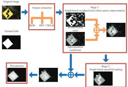
Fig. 3: Diagram of the proposed salient object detection method.
In this section, we will describe the proposed salient object detection system. The diagram of the proposed method is illustrated in Fig. 3. The proposed system consists of four components: feature extraction; graph-based weighted joint robust sparse representation; graph-based manifold ranking; and post processing. Each part is elaborated below.
A. Feature Extraction
(a)
(b)
Fig. 4: Graph G1 at the first stage. (a) Original image. (b) GraphG1. Any node is connected to its neighbors, as shown in the area delineated by the green curve. Besides, the boundary nodes are selected as the background seed nodes, as shown by the nodes marked by blue color in (b).
features of RGB, HSV, and CIELab. Traditionally, per-pixel feature vector is converted to per-superpixel feature vector through averaging. However, this appears to perform well only if the scene is characterized by simple color information and texture, whereas in nonhomogeneous regions and complex scenes it fails to maintain robustness. Instead, we obtain the per-superpixel feature vector by
xi=
1
C
ni
∑
j=1
wjifj, (1)
where fj ∈Rm×1 is the feature vector of the pixelj within the superpixel i.ni is the number of pixels in the superpixel
i. C is a normalization constant. wji is the distance weight and is computed by
wji= exp
(
∥pj−pi∥22
2∗σ2
p
)
, (2)
wherepi andpj are the positions of the centers of the super-pixeliand the pixeljwithin the superpixeli, respectively.σp is a scalar, and is set to√2.
Finally, horizontally stacking the feature vectors of all superpixels produces the feature matrix X ∈Rm×N for the input image, i.e., X = [x1, x2, . . . , xN]∈Rm×N.
B. Stage 1: Graph-based Weighted Joint Robust Sparse Rep-resentation
In this section, we will describe the first stage of the proposed method, which consists of three parts: graph con-struction, weighted joint robust sparse representation model, and saliency measure.
1) Graph Construction: At the first stage, an undirected
regular graph is constructed G1= (V1,E1), where the nodes
V1 are the superpixels. As illustrated in Fig. 4(b), each
node is connected to its neighboring ones, which considers a spatial consistency within a local neighborhood, i.e., the
adjacently spatial consistency, in light of the observation that
a superpixel and its neighbors are likely to share similar appearance and thereby similar saliency values. In addition, the image boundary nodes, as shown in Fig. 4(b), are selected as the background seed nodes according to the boundary prior [19].
[image:4.612.95.254.56.132.2](a) (b) (c) (d) (e) (f)
Fig. 5: Illustrations of the proposed WJRSR against the traditional manifold ranking based and SR based methods. (a) Original images; (b) MR; (c) SR; (d) RSR; (e) Proposed WJRSR; (f) Ground truth. The boundary regions are selected as the background seed nodes (background dictionary).
The edge weights are defined as
wG1 ij =
exp
(
−∥xi−xj∥
2 2
2σ2
G1
)
, if i and j are connected
0, otherwise.
,
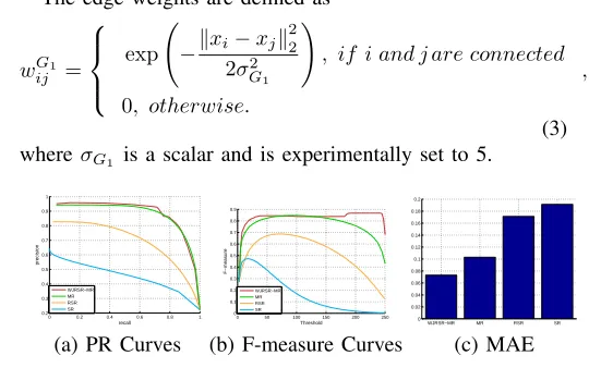
(3) whereσG1 is a scalar and is experimentally set to 5.
0 0.2 0.4 0.6 0.8 1 0.2
0.3 0.4 0.5 0.6 0.7 0.8 0.9 1
recall
precision
WJRSR−MR MR RSR SR
(a) PR Curves
0 50 100 150 200 250 0
0.1 0.2 0.3 0.4 0.5 0.6 0.7 0.8 0.9
Threshold
F−measure
WJRSR−MR MR RSR SR
(b) F-measure Curves
WJRSR−MR MR RSR SR 0
0.02 0.04 0.06 0.08 0.1 0.12 0.14 0.16 0.18 0.2
(c) MAE
Fig. 6:Quantitative comparisons of the proposed WJRSR model with MR, RSR, and SR models on MSRA10K. (a) PR Curves; (b) F-measure Curves; (c) Mean Absolute Error (MAE). The MSRA10K dataset, PR, F-measure, and MAE evaluation metrics will be discussed in Section VI.
2) Weighted Joint Robust Sparse Representation Model for
the Computing of Saliency Values: Given the graph G1, the
way the saliency values of nodes are calculated is of great importance. Most graph-based saliency detection methods adopt manifold ranking to compute the saliency value of each node [6]–[8], [21]. However, manifold ranking is sensitive to the initial saliency values of nodes. It becomes unreliable when the seed nodes are mixed with noise, producing undesirable detection results. For example, as shown in the first two rows of Fig. 5(b), when parts of foregrounds reach the image boundary, manifold ranking fails at identifying the foreground objects.
[image:4.612.303.573.232.401.2]appears around the image boundary. Besides, when applied to the detection of salient objects, the RSR model possesses higher distinctiveness between the foreground objects and their backgrounds than the SR model. As shown in the last two rows of Fig. 5(d) and (e), the salient objects can be more uniformly highlighted and the background noise can also be better suppressed by the RSR model, as opposed to the SR model. It can be also found from Fig. 6 that the RSR model achieves better performance than the traditional SR model. Besides, the proposed WJRSR model performs better than the previous MR and RSR models.In the following, we will describe the WJRSR model in detail.
Joint Robust Sparse Representation (JRSR) Model.
Based on the adjacently spatial consistency defined by the graph G1, the superpixel to be tested and its neighbors share
similar appearances and thereby will have more or less the same saliency values. This implies that their representation coefficients when sparsely reconstructed using the same dic-tionary will look similar. As a result, a row-sparsity constraint is imposed on the representation coefficients of the superpixel to be tested and its neighbors, so that only few rows of the representation coefficients matrix are zero. Besides, the background seed nodes are taken as the background dictionary in the RSR model, which promotes the global contrast.
We horizontally stack the feature vectors of each su-perpixel to be tested and its neighbors, i.e., Xi = [xi, xi−1, xi−2, . . . , xi−Ni], where xi−1, xi−2, . . . , xi−Ni are the feature vectors of the neighboring superpixels belonging to the superpixel i. Based on the above discussions, we formulate a joint robust sparse representation (JRSR) model for computing the saliency value of the superpixeli as:
min
Zi,Ei
Zi1,2+λEi2,1
s.t. Xi=DZi+Ei
. (4)
Here,Dis the background dictionary, i.e., the background seed nodes. Zi and Ei are the representation coefficients matrix and reconstruction errors matrix, respectively. Zi
1,2 is the l1,2- norm of Zi, and defined as Zi1,2 =
∑
j
Zi(j,:)2,
whereZi(j,:)is thejth row ofZi.Zi(j,:)
2is thel2-norm
of Zi(j,:). Ei2,1 is the l2,1- norm ofEi, and defined as
Ei2,1=∑
k
√∑
j
(Ei(j, k))2, where Ei(j, k)is the (j, k)th
entry of Ei. Similar to Xi, Zi and Ei are the matrices which horizontally stack the representation coefficients vectors and reconstruction errors vectors of the superpixel i and its neighbors, respectively, i.e., Zi = [z
i, zi−1, zi−2, . . . , zi−Ni] and Ei = [e
i, ei−1, ei−2, . . . , ei−Ni]. Z
i
1,2 achieves the
adjacently spatial consistency, and enforces the superpixel
to be tested and its adjacent superpixels to be with similar representation coefficients under the same dictionary.
Weighted JRSR (WJRSR) Model. As defined by Eq.
(4), the representation coefficients for each superpixel and its neighboring ones are assumed to be similar if the “row-sparsity” constraint is directly imposed on the coefficient matrix in the JRSR model. This assumption seems reasonable for the homogeneous regions, but it is no longer valid for those
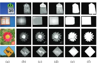
[image:5.612.370.504.54.156.2](a) (b) (c) (d)
Fig. 7: Illustrations of the superiority of the WJRSR model over the JRSR model. (a) Original images; (b) Proposed JRSR model in Eq. (4); (c) Proposed WJRSR model in Eq. (5); (d) Ground truth.
nonhomogeneous regions, especially for the object boundaries. For example, as shown in Fig. 7(b), some backgrounds (fore-grounds) are mistakenly labeled as foregrounds (back(fore-grounds) at the object boundary. To achieve both the diversity for the nonhomogeneous regions and the consistency for the homo-geneous regions, we introduce a weight matrixQi, leading to a weighted JRSR (WJRSR) model:
min
Zi,Ei
ZiQi1,2+λEi2,1
s.t. Xi=DZi+Ei
, (5)
whereQi is defined as
Qi=
1 0 · · · 0
0 qi−1 · · · 0
..
. ... . .. ...
0 0 · · · qi−Ni
. (6)
Here,qi−k, k= 1,2, . . . , Ni is the feature similarity measure of the superpixel i and its neighboring superpixel k, and is computed by Eq. (3). Therefore, the row-sparsity constraint enforces the representation coefficients associated with each superpixel to be tested and its neighboring ones to be similar in case they share similar appearance, but not vice versa. This not only imposes the consistency for the homogeneous regions, but also preserves the diversity for the nonhomogeneous regions. This is different from the JRSR model defined by Eq. (4). Thanks to this scheme, we can observe from Fig. 7(c) that the WJRSR model accurately detects the foreground regions and background regions even at the object boundary.
Moreover, the proposed WJRSR model is different from WSC [43]. First, WSC [43] is based on the SR model, while our proposed WJRSR model is based on the RSR model, which is superior to the SR model for salient object detection (as discussed in Fig. 5). Secondly, the penalty weights in WSC [43] are defined to be inversely proportional to the appearance similarities between the superpixels to be tested and the dictionary atoms. In contrast, our proposed WJRSR model defines the weights as the appearance similarities between the superpixels to be tested and their adjacently spatial neighbors. Thirdly, WSC [43] computes the saliency value of each superpixel independently, while our proposed WJRSR model considers the adjacently spatial consistency
(a) (b) (c) (d)
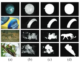
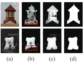
Fig. 8: Illustrations of the superiority of the proposed WJRSR model over WSC [43]. (a) Original images; (b) WSC; (c) WJRSR; (d) Ground truth.
obtains incomplete detection results, whereas our proposed WJRSR model gets more wholeness of the salient objects. It can also be obviously found from the last two rows of Fig. 8 that our proposed WJRSR model achieves better foreground uniformity than WSC [43] does.
Optimization. For the sake of clarity, we remove the
subscript index of the matrices in Eq. (4), and the WJRSR model in Eq. (5) can be rewritten as
min
˜
Z,E˜
Z˜Q˜
1,2
+λE˜
2,1
s.t.X˜ =DZ˜+ ˜E
. (7)
This optimization model is convex and can be solved efficiently. We first convert it to the following equivalent problem:
min
J,Z,˜E˜∥
J∥1,2+λE˜ 2,1
s.t.X˜ =DZ˜+ ˜E,
˜
ZQ˜=J
. (8)
In this paper, to optimize the objective function defined in Eq. (8), we adopt the ADMM method [44] which minimizes the following augmented Lagrange function:
L=∥J∥1,2+λE˜ 2,1+
⟨
Y1,X˜−DZ˜−E˜
⟩
+
⟨
Y2,Z˜Q˜−J
⟩
+µ
2
(
X˜ −DZ˜−E˜2
F
+Z˜Q˜−J
2
F
),
(9)
where Y1 and Y2 are Lagrange multipliers, and µ > 0 is a
penalty parameter.
The optimization procedure is outlined in Algorithm 1. The detailed solving process is shown in Supplementary Material.
Through Algorithm 1, we can obtain the optimal represen-tation coefficients matrixZi∗and reconstruction errors matrix
Ei∗ for Xi. Then, the optimal z∗
i ande∗i are extracted from
Zi∗ and Ei∗, respectively. Similarly, we are able to get the optimal representation coefficients vectors and reconstruction errors vectors corresponding to the other superpixels. Thus, we can obtain the optimal representation coefficients matrix
Z∗ = [z1∗, z2∗, . . . , zN∗] and the optimal reconstruction errors matrix E∗= [e∗1, e∗2, . . . , e∗N] for the input image.
Algorithm 1 Solving the optimization model in Eq. (9).
Input: Feature matrixX˜, weight matrixQ˜, and parameterλ.
Output: Z˜ andE˜.
1: intialize: Z˜ = 0, E˜ = 0, Y1 = 0, Y2 = 0, µ = 1,
µmax= 1010, andρ= 1.1.
2: repeat
3: Fix the others and update J:
J = arg min
J
1
µ∥J∥1,2+
1 2
J−( ˜ZQ˜+1
µY2)
2
F
.
4: Fix the others and update Z˜ by updating each column of Z˜:
˜
zk= (A+ ˜Qi,iI)−1ci,
where A = ˜Q−1DTD, Q˜i,i is the (i, i) entry of Q˜,
and ci is the ith column of the matrix C, which is formulated as
C= ˜Q−1
[
DT
(
˜
X−E˜+Y1
µ
)
+ ˜Q(J−Y2
µ)
]
.
5: Fix the others and update E˜:
˜
E= arg min
˜
E
λ
µ∥E∥2,1+
1 2
E˜−
(
˜
X−DZ˜+Y1
µ
) 2
F
.
6: Update the multipliers:
Y1=Y1+µ
(
˜
X−DZ˜−E˜
)
.
Y2=Y2+µ
(
˜
ZQ˜−J
)
.
7: Update the parameterµ: µ= min (ρµ, µmax)
8: untilConvergence:X˜ −DZ˜−E˜→0andZ˜Q˜−J →0
3) Saliency Measure: In this part, we will describe how
we define the saliency measures based on the reconstruction errors and representation coefficients.
Saliency Measure Based on Reconstruction Errors.
Giv-en a background dictionary D, each column of the optimal sparse errors matrixE∗may contain the salient information of each superpixel that is distinct from the background. Generally, a superpixel will be more salient if it has larger reconstruction errors with respect to the background dictionary. Hence, we define the reconstruction errors based saliency measure
salE(i)for the superpixel ias
salE(i) = 1−exp
(
−∥E∗(:, i)∥
2 2
2σ2
E
)
, (10)
whereσEis a scalar parameter and is experimentally set to 1.
Saliency Measure Based on Representation Coefficients.
[image:6.612.310.568.85.407.2]background superpixel but higher contrast with the foreground superpixel. Based on the observations, we define the repre-sentation coefficients based saliency measure salZ(i) for the superpixel ias
salZ(i) = 1−exp
(
−∥Z∗(:, i)∥
2 2
2σ2Z
)
, (11)
whereσZ is a scalar and is experimentally set to √
2.
0 10 20 30 40 50
−0.1 0 0.1 0.2 0.3 0.4 0.5 0.6 0.7 0.8 0.9
index
value
(a)
0 10 20 30 40 50
−3 −2 −1 0 1 2 3 4
index
value
[image:7.612.357.518.56.132.2](b)
Fig. 9: Comparisons of representation coefficients between (a) background superpixel and (b) foreground superpixel.
The two saliency measures salE and salZ are integrated, resulting in the saliency measure for the superpixel i
salE Z(i) =α∗salE(i) + (1−α)∗salZ(i), (12)
where α ∈ (0,1) is a balance weight and is experimentally set to 0.2.
The pixel-level saliency map is obtained by equaling the saliency value of each pixel to that of its corresponding superpixel. In order to suppress the noise, the object-based Gaussian model [4], [5] is further applied to refine the saliency detection results. In the subsequent processing at the second stage, we again transform the pixel-level saliency map to superpixel-level saliency map. Each superpixel achieves its saliency value by averaging the saliency values of the pixels within it. The refined results are denoted assalG1.
C. Stage 2: Graph-based Manifold Ranking
In this section, we will describe the second stage of the proposed method, which consists of graph construction and graph-based manifold ranking.
1) Graph Construction: The coarse detection results
ob-tained from the first stage help to locate the potential back-ground region RB and foreground region RF if a low threshold threlow and a high threshold threhigh are set. Those superpixels with saliency values lower than threlow are labeled as background ones, while those supeprixels with saliency values higher thanthrehigh are labeled as foreground ones. To ensure the accuracy of the potential background and foreground regions detection, we set threlow = 0.8 ∗
mean(salG1)andthre
high= 2∗mean(salG1). Based on the potential background and foreground regions, we construct a novel undirected graph G2 = (V2,E2), where nodes are the
superpixels. As shown in Fig. 10(b), the edges of this graph are composed of three parts:
E1
2: Each node is connected to its neighboring nodes.
E2
2: Any pairs of the potential background nodes are
con-nected.
(a)
(b)
Fig. 10: GraphG2at the second stage. (a) Original image. (b) GraphG2. The nodes marked by red color represent the foreground superpixels and the nodes marked by blue color represent background superpixels. In this graph, each node is connected to its neighboring nodes, as shown in the area delineated by the green curve. Besides, any pairs of the red nodes are connected, and any pairs of the blue nodes are connected, which are not marked for clarity.
E3
2: Any pairs of the potential foreground nodes are
con-nected.
E1
2 considers the local consistency within a local
neighbor-hood, i.e., theadjacently spatial consistency, which plays the same role as that employed in the graphG1 at the first stage.
E2
2 treats any pairs of RB to be adjacent, which enforces a consistency among the potential background nodes, resulting in the background uniformity. E3
2 treats any pairs of RF to be adjacent, which enforces consistency among the potential foreground nodes, leading to the foreground uniformity. E2 2
and E3
2 impose the regionally spatial consistency within the
background candidates and within the foreground candidates, respectively. Furthermore, combining E22 and E32 can addi-tionally enhance the discrimination between background and foreground, thus improving the separation of the foreground from the background. Similar toG1, the edge weight between
two nodes onG2 is defined as
wG2 ij =
exp
(
−∥xi−xj∥
2 2
2σ2
G2
)
, if i and j are connected
0, otherwise.
.
(13) Here,σG2 is a scalar and is experimentally set to
√
8, which is different from the first stage.
2) Graph-based Manifold Ranking: At this stage, we
ini-tialize the saliency value of each nodey = [y1, y2, . . . , yN] T
with the saliency value of the coarse detection conducted in the first stage, i.e.,
yi=salG1(i), i= 1,2, . . . , N. (14)
Given the weight matrixWG2 =
[
wG2 ij
]
N×N, we can obtain the degree matrix DG2 =diag(d1, d2, . . . , d
N), where di =
∑
i
wG2
ij . Let f be the ranking function assigning rank values
f = [f1, f2, . . . , fN] T
. This can be obtained by solving the following minimization problem:
f∗= arg min
f
1 2
N
∑
i,j=1 wG2
ij
fi √
di −√fj
dj
2
2
+β
2
N
∑
i=1
∥fi−yi∥
2 2
[image:7.612.53.302.111.257.2]whereβ is a controlling parameter. The optimized solution is given in [45] as:
f∗=(DG2−γWG2)−1y, (16)
whereγ= 1
1+β, andγ is set to 0.99.
Then, the saliency value of the superpixel i at the second stage is
salG2(i) =f∗(i). (17)
Furthermore, salG1 and salG2 may contain noise in both
foreground and background regions, we integrate the detection results of the two stages to complement each other by
salG1 G2= sal
G1+salG2
2 . (18)
D. Post Process
The pixel-level saliency map is first obtained fromsalG1 G2
by setting the saliency value of each superpixel to that of the pixels within the superpixel. An enhanced pixel-level saliency map salenhance is then obtained by using the following enhancement function:
g(x) =x+sgn(x−ε)∗exp(− x−ε
2σ2
enhance
), (19)
where ε is an adaptive threshold based on the Otsus binary threshold method [46].σenhance is a predefined parameter to control the level of contrast, and is set to 1. sgn(·)is a sign function. Here,xdenotes the saliency value of a pixel.
Generally, salient object detection is essentially a binary segmentation problem [47] that extracts the entire salient objects from the background. To advance the binary segmen-tation, we apply the Max-Flow method [48] on salenhance
to generate a foreground mask salM F. Similarly, considering that the binary saliency map salM F may also contain noise in both foreground and background regions, we get the final saliency map as formulated by
salpost =sal
enhance+salM F
2 . (20)
It should be noted that the post process can actually improve the performance of the proposed method to some extent. However, this depends on the pre-detection results of the proposed two-stage graphs before the post process. In other words, the post process will improve the performance in case the pre-detection results are good, but will degrade the performance otherwise. For example, as shown in Fig. 11, the post-process operation improves the performance when the proposed two-stage graphs achieve good detection results (as shown in the first two rows of Fig. 11), but degrade the performance when the proposed two-stage graphs achieve unsatisfactory detection results (as shwon in the last two rows of Fig. 11).
Moreover, compared with the post process in [20], [49], the proposed post-process can better improve the performance of salient object detection. As shown in Fig. 12, some foreground regions are suppressed instead of being promoted to some extent by the post-process in [20], [49]. While the foreground regions and the background regions are further promoted and suppressed, respectively, by our proposed post-process.
[image:8.612.369.507.53.160.2](a) (b) (c) (d)
Fig. 11:Illustrations of the improvements of the post-process for the per-formance of the proposed method. (a) Original images; (b) Saliency maps obtained by the proposed two-stage graphs without post-process; (c) Saliency maps refined by the post-process; (d) Ground truth.
[image:8.612.368.506.214.335.2](a) (b) (c) (d) (e)
Fig. 12:Illustrations of superiority of the proposed post-process. (a) Original images; (b) Saliency maps obtained by the proposed two-stage graphs without post-process; (c) Saliency maps refined by the post-process in [20], [49]; (d) Saliency maps refined by the proposed post-process (e) Ground truth.
E. Summary
To recapitulate, the proposed salient object detection method is summarized as follows:
(1) Extract features for each superpixel by Eq. (1); (2) Compute the coarse saliency mapsalG1 at the first stage;
(3) Compute the saliency mapsalG2 at the second stage;
(4) Compute the integrated saliency mapsalG1 G2;
(5) Obtain the final saliency map salpost via post process operations.
Fig. 13 illustrates the saliency detection results obtained by the main phases of the proposed method. As shown in Fig. 13(d), most background and foreground regions are identified in the first stage, and they become more uniform and discriminative through the refinement in the second stage (See the example in Fig 13(e)).
F. Complexity Analysis
Firstly, the computational complexity at the first stage can be analyzed as follows: suppose the data matrixXand dictionary
Dare with the sizes ofm×N andm×K, respectively. Then, the coefficients matrix Z has size of K×N. As discussed in [42], the computational complexity of Algorithm 1 at the first stage is mainly determined by the computation burden of updating the matrix Z. Theoretically, the computational complexity of Algorithm 1 is O(rK3N), where r is the
number of iterations needed for convergence3. It demonstrates 3Note that we assume that all the iterations for updating Zi, i =
(a) (b) (c) (d) (e) (f) (g) (h)
Fig. 13:Saliency maps obtained by the main phases of the proposed method. (a) Original image; (b)-(d) Saliency maps obtained from the first stage: (b) based on the reconstruction errors; (c) based on the representation coefficients; (d) by fusing (b) and (c); (e) Saliency maps obtained from the second stage; (f) Saliency maps by fusing (d) and (e); (g) Final saliency maps via post process operations; (h) Ground truth.
that the number of dictionary atoms K has a greater impact on the computational complexity of the proposed Algorithm 1 than the other parameters. In the proposed method, K is set to the number of boundary superpixels (about 49) and is far smaller than the total number of superpixels N (about 200). This makes the computational cost of the proposed Algorithm 1 acceptable.
Next, we will discuss the computational complexity at the second stage. The computational complexity of the manifold ranking model at the second stage mainly depends on the matrix inverse operation in Eq. (16). The matrices DG2 and WG2 are both with the size of N ×N. The computational
complexity of the manifold ranking model is thus O(N3).
Therefore, the total computational complexity of our proposed method is O(rK3N) +O(N3).
IV. EXPERIMENTS ANDANALYSIS
In this section, a number of experiments are conducted to validate the effectiveness and superiority of the proposed salient object detection method.
Datasets.We evaluate the proposed method on three
bench-mark datasets, including MSRA10K [50], ECSSD [51], and DUT-OMRON [6], [7]. MSRA10K [50] contains 10000 im-ages with simple scene, most of which contain a single object with high contrast to background. ECSSD [51] contains 1000 images with structurally complex scene. Most images in this dataset contain multiple objects belonging to various categories. DUT-OMRON [6], [7] contains 5168 images with cluttered background, most of which have one or more objects with different scales and locations.
Evaluation metrics. Multiple widely used evaluation
met-rics are used to evaluate the proposed method, including precision-recall curve [52], F-measure [52], mean absolute error (MAE) [53]. Here, the precision value is defined as the ratio of salient pixels correctly assigned to all pixels of the extracted regions, while the recall value refers to the percentage of detected salient pixels with respect to the ground truth data. For a saliency map, we generate a set of binary images by using different thresholding values in the range of
[0,1]. The precision/recall pairs of all the binary maps are computed to plot the precision-recall curve [52]. F-measure is used as the overall performance measure:
F= (1 +β
2)∗precision∗recall
β2∗precision+recall , (21)
where β2 = 0.3 as suggested in [52] to emphasize the
precision. The MAE computes the average difference between the saliency map and the ground truth [53].
A. Parameters Setup
The superpixel number N has an important impact on the performance of the proposed method. Besides, the parameterλ
in Eq. (4) balances the two constraints of the proposed WJRSR model. We set the two important parameters by fixing one and tuning the other on ECSSD within the first stage of our proposed method.
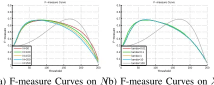
It can be seen from Fig. 14(a) that WJRSR gets good performance whenN = 50,100,150, and 200. However, the F-measure curve gets high values over a suddenly narrow range when N = 250. This indicates that the detection algorithm poorly distinguishes the foreground from the back-ground, which would result in inaccurate location of potential foreground and background regions. Considering that more superpixels are beneficial to detecting the salient object in the case of nonhomogeneous regions and complex scene, we set
N = 200.
From Fig. 14(b), it can be viewed that WJRSR performs similarly when λ = 0.01,0.1,1 and 10. But the F-measure curve is obviously poor when λ = 100, which degrades the localization accuracy of potential foreground and background regions. In the following experiments, we setλ= 0.1.
0 50 100 150 200 250 0
0.1 0.2 0.3 0.4 0.5 0.6 0.7 0.8 0.9
Threshold
F−measure
F−measure Curve
N=50 N=100 N=150 N=200 N=250
(a) F-measure Curves on N
0 50 100 150 200 250 0
0.1 0.2 0.3 0.4 0.5 0.6 0.7 0.8 0.9
Threshold
F−measure
F−measure Curve
lamda=0.01 lamda=0.1 lamda=1 lamda=10 lamda=100
[image:9.612.331.545.387.472.2](b) F-measure Curves on λ
Fig. 14: Illustrations of parameters setting. It is noted that the F-measure curves forλ= 0.01,λ= 1, andλ= 10overlap in (b).
B. Performance Comparisons on Each Stage
Fig. 15 provides the detection results of each stage in our proposed method on ECSSD. It is obvious from Fig. 15 that compared with “Stage 1”, “Stage 2” achieves higher PR curve when recall value is greater than 0.4 (Fig. 15(a)), much higher and wider measure curve (Fig. 15(b)), and higher mean F-measure value (Fig. 15(c)). Besides, since that there exists a complementarity between “Stage 1” and “Stage 2”, the performance is further improved by integrating the detection results of the two stages. And thus “Stage 1 + Stage 2” obtains better performance than “Stage 1” and “Stage 2”, which can be easily seen from Fig. 15. Finally, a simple but effective post process is performed on “Stage 1 + Stage 2” to further promote performance.
2” with much better foreground uniformity and background suppression, which is easily seen from Fig. 16(c). Besides, it can be found from Fig. 16(d) that “Stage 1 + Stage 2” makes “Stage 1” and “Stage 2” complement each other to achieve more accurate saliency maps. The detection results are more close to ground truth with the help of the post process.
0 0.2 0.4 0.6 0.8 1 0.2
0.3 0.4 0.5 0.6 0.7 0.8 0.9 1
recall
precision
Precision and Recall (PR) Curve
Stage 1 Stage 2 Stage 1 + Stage 2 Post
(a) PR Curves
0 50 100 150 200 250 0
0.1 0.2 0.3 0.4 0.5 0.6 0.7 0.8
Threshold
F−measure
F−measure Curve
Stage 1 Stage 2 Stage 1 + Stage 2 Post
(b) F-measure Curves
stage 1 stage 2 stage 1+stage 2 post 0.64
0.66 0.68 0.7 0.72 0.74 0.76 0.78 0.8
Mean F−measure Value
[image:10.612.358.518.53.157.2](c) Mean F-measure
Fig. 15: Performance comparisons of each stage on ECSSD. “Stage 1” represents the saliency map salG1 obtained from the first stage. “Stage 2”
represents the saliency mapsalG2obtained from the second stage. “Stage 1 +
Stage 2” represents the integrated saliency mapsalG1G2. “Post” represents
the final saliency mapsalpost. Mean F-measure value is computed with an
adaptive threshold, i.e., thre= W2×H∑Wi=1∑Hj=1S(i, j), whereS(i, j) represents the saliency value of the(i, j)-th pixel in the saliency mapS.
C. Comparisons with State-of-the-art Methods
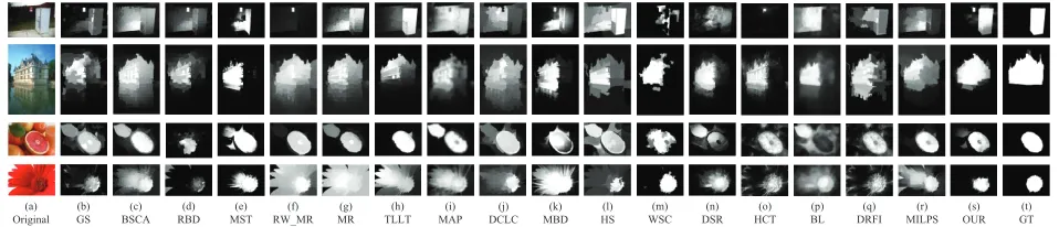
In this section, we validate the effectiveness and superiority of the proposed method via visual and quantitative compar-isons with 20 state-of-the-art methods, including MST [20], TLLT [18], BSCA [54], DSR [5], WSC [43], MBD [49], MR [7], RBD [55], HS [51], PCA [56], TD [57], GC [58], DCLC [59], RW MR [21], MAP [60], GS [19], HCT [61], BL [62], DRFI [63], and MILPS [64].Among these methods, GS [19], BSCA [54], RBD [55], MST [20], RW MR [21], MR [7], TLLT [18], MAP [60], and DCLC [59] are graph based state-of-the-art methods. Specifically, GS [19], BSCA [54], RBD [55], and MST [20] are one-stage based methods. RW MR [21], MR [7], TLLT [18], MAP [60], and DCLC [59] are two-stage scoring based methods. The other methods, i.e., MBD [49], HS [51], WSC [43], DSR [5], HCT [61], BL [62], DRFI [63], MILPS [64], are other state-of-the-art methods.
1) Visual Comparisons on Several Types of Images: To
efficiently validate the effectiveness and superiority of the proposed method, we compare the proposed method with the state-of-the-art methods on several types of images. Fig. 17 - Fig. 22 show the visual comparisons on different methods for those images with a single object, multiple objects, large object, object touching the image borders, similar appearance between background and foreground, and complex scene, respectively. Most methods deliver good results in the simple cases, such as those images with a single object (in Fig. 17), but fail to produce satisfactory results in more complex cases. In contrast, the proposed method can not only extract the salient object accurately for those images with a single object, but also offers pretty good detection in complex scenes. Especially, it can be found that the proposed two-stage graphs achieves much better performance in foreground uniformity as well as background suppression.
For those images with multiple objects (in Fig. 18), our pro-posed method can extract all the salient objects. Especially, as shown in the second and fourth rows of Fig. 18, those multiple
(a) (b) (c) (d) (e) (f)
Fig. 16:Detection results of each stage. (a) Original images; (b) Stage 1; (c) Stage 2; (d) Stage 1 + Stage 2; (e) Post; (f) Ground truth. Please refer to Fig. 15 for the explanations of “Stage 1”, “Stage 2”, “Stage 1 + Stage 2”, and “Post”.
salient objects can also be well separated from background by using our proposed method. For those images with large objects (in Fig. 19), our proposed method is able to detect the entire salient object, whereas most of the other methods just detect parts of the salient objects. For those images with salient object touching the image borders (in Fig. 20), it is difficult to segment the entire object, especially for those boundary prior based methods, i.e., BSCA [54], RW MR [21], MR [7], RBD [55], MBD [49], WSC [43], DSR [5], and MST [20]. In contrast, our proposed method can still extract the entire object, which may owe to the WJRSR model at our first stage. For those images with similar appearance between background and foreground (in Fig. 21), our proposed method can successfully separate the foreground from the background. On the contrary, such similar appearances confuse most of the other algorithms. For those images with complex scene (in Fig. 22), our proposed method can identify the salient object pretty accurately, but most of the other methods fail, especially in the second row of Fig. 22.
2) Quantitative Comparisons: Fig. 23 provides the PR and
[image:10.612.51.306.57.213.2] [image:10.612.55.305.133.212.2](a) Original
(i) MAP (f)
RW_MR (g) MR (c)
BSCA
(h) TLLT
(o) HCT
(p) BL
(q) DRFI
(r) MILPS (e)
MST
(t) GT (s) OUR (d)
RBD
(n) DSR (m) WSC (b)
GS
(j) DCLC
(k) MBD
[image:11.612.67.547.57.154.2](l) HS
Fig. 17:Visual comparisons on different methods for those images with a single object. (b)-(e) are one-stage based methods. (f)-(j) are two-stage scoring based methods. (k)-(r) are other state-of-the-art methods.
(a) Original
(i) MAP (f)
RW_MR (g) MR (c)
BSCA
(h) TLLT
(o) HCT
(p) BL
(q) DRFI
(r) MILPS (e)
MST
(t) GT (s) OUR (d)
RBD
(n) DSR (m) WSC (b)
GS
(j) DCLC
(k) MBD
[image:11.612.66.551.193.276.2](l) HS
Fig. 18:Visual comparisons on different methods for those images with multiple objects. (b)-(e) are one-stage based methods. (f)-(j) are two-stage scoring based methods. (k)-(r) are other state-of-the-art methods.
(a) Original
(i) MAP (f)
RW_MR (g) MR (c)
BSCA
(h) TLLT
(o) HCT
(p) BL
(q) DRFI
(r) MILPS (e)
MST
(t) GT (s) OUR (d)
RBD
(n) DSR (m) WSC (b)
GS
(j) DCLC
(k) MBD
[image:11.612.68.547.311.422.2](l) HS
Fig. 19:Visual comparisons on different methods for those images with large object. (b)-(e) are one-stage based methods. (f)-(j) are two-stage scoring based methods. (k)-(r) are other state-of-the-art methods.
(a) Original
(i) MAP (f)
RW_MR (g) MR (c)
BSCA
(h) TLLT
(o) HCT
(p) BL
(q) DRFI
(r) MILPS (e)
MST
(t) GT (s) OUR (d)
RBD
(n) DSR (m) WSC (b)
GS
(j) DCLC
(k) MBD
(l) HS
Fig. 20:Visual comparisons on different methods for those images with object touching the image borders. (b)-(e) are one-stage based methods. (f)-(j) are two-stage scoring based methods. (k)-(r) are other state-of-the-art methods.
(a) Original
(i) MAP (f)
RW_MR (g) MR (c)
BSCA
(h) TLLT
(o) HCT
(p) BL
(q) DRFI
(r) MILPS (e)
MST
(t) GT (s) OUR (d)
RBD
(n) DSR (m) WSC (b)
GS
(j) DCLC
(k) MBD
(l) HS
[image:11.612.68.543.459.577.2] [image:11.612.67.546.617.720.2](a) Original (i) MAP (f) RW_MR (g) MR (c) BSCA (h) TLLT (o) HCT (p) BL (q) DRFI (r) MILPS (e) MST (t) GT (s) OUR (d) RBD (n) DSR (m) WSC (b) GS (j) DCLC (k) MBD (l) HS
Fig. 22:Visual comparisons on different methods for those images with complex scene. (b)-(e) are one-stage based methods. (f)-(j) are two-stage scoring based methods. (k)-(r) are other state-of-the-art methods.
0 0.2 0.4 0.6 0.8 1
0.2 0.3 0.4 0.5 0.6 0.7 0.8 0.9 1 recall precision OUR MST [20] RBD [55] MR [7] DCLC [59] RW_MR [21] MAP [60] GS [19] TLLT [18] BSCA [53]
0 0.2 0.4 0.6 0.8 1
0.2 0.3 0.4 0.5 0.6 0.7 0.8 0.9 1 recall precision OUR TD [57] GC [58] HCT [61] BL [62] DSR [5] WSC [43] MBD [54] HS [50] PCA [56] DRFI [63] MILPS [64]
0 50 100 150 200 250
0 0.1 0.2 0.3 0.4 0.5 0.6 0.7 0.8 0.9 1 Threshold F−measure OUR MST [20] RBD [55] MR [7] DCLC [59] RW_MR [21] MAP [60] GS [19] TLLT [18] BSCA [53]
0 50 100 150 200 250
0 0.1 0.2 0.3 0.4 0.5 0.6 0.7 0.8 0.9 1 Threshold F−measure OUR TD GC MAP HCT DSR WSC MBD HS PCA DRFI MILPS (a)
0 0.2 0.4 0.6 0.8 1
0 0.1 0.2 0.3 0.4 0.5 0.6 0.7 0.8 0.9 1 recall precision OUR MST [20] RBD [55] MR [7] DCLC [59] RW_MR [21] MAP [60] GS [19] TLLT [18] BSCA [53]
0 0.2 0.4 0.6 0.8 1
0.2 0.3 0.4 0.5 0.6 0.7 0.8 0.9 1 recall precision OUR TD [57] GC [58] HCT [61] BL [62] DSR [5] WSC [43] MBD [54] HS [50] PCA [56] DRFI [63] MILPS [64]
0 50 100 150 200 250
0 0.1 0.2 0.3 0.4 0.5 0.6 0.7 0.8 0.9 Threshold F−measure OUR MST [20] RBD [55] MR [7] DCLC [59] RW_MR [21] MAP [60] GS [19] TLLT [18] BSCA [53]
0 50 100 150 200 250
0 0.1 0.2 0.3 0.4 0.5 0.6 0.7 0.8 0.9 Threshold F−measure OUR TD [57] GC [58] HCT [61] BL [62] DSR [5] WSC [43] MBD [54] HS [50] PCA [56] DRFI [63] MILPS [64] (b)
0 0.2 0.4 0.6 0.8 1
0 0.1 0.2 0.3 0.4 0.5 0.6 0.7 0.8 0.9 recall precision OUR MST [20] RBD [55] MR [7] DCLC [59] RW_MR [21] MAP [60] GS [19] TLLT [18] BSCA [53]
0 0.2 0.4 0.6 0.8 1
0 0.1 0.2 0.3 0.4 0.5 0.6 0.7 0.8 0.9 recall precision OUR TD [57] GC [58] HCT [61] BL [62] DSR [5] WSC [43] MBD [54] HS [50] PCA [56] DRFI [63] MILPS [64]
0 50 100 150 200 250
0 0.1 0.2 0.3 0.4 0.5 0.6 0.7 0.8 Threshold F−measure OUR MST [20] RBD [55] MR [7] DCLC [59] RW_MR [21] MAP [60] GS [19] TLLT [18] BSCA [53]
0 50 100 150 200 250
[image:12.612.77.538.182.469.2]0 0.1 0.2 0.3 0.4 0.5 0.6 0.7 0.8 Threshold F−measure OUR TD [57] GC [58] HCT [61] BL [62] DSR [5] WSC [43] MBD [54] HS [50] PCA [56] DRFI [63] MILPS [64] (c)
Fig. 23:PR and F-measure curves on different methods for (a) MSRA10K, (b) ECSSD, and (c) DUT-OMRON.
D. Improvement of State-of-the-art Methods
Fig. 24 illustrates some improved results by integrating our second stage into different state-of-the-art salient object detection methods. The coarse detection results used in our proposed second stage are the detection results of the original methods. It is obvious that those improved methods achieve higher F-measure values over a wider range and smaller MAE scores than their corresponding original methods.
For better understanding, Fig. 25 shows some visual ex-amples to illustrate the improved results of our proposed second stage on some state-of-the-art methods. More visual examples can be found in the Supplementary Material. It can be easily found that our second stage improves the state-of-the-art methods with much better foreground uniformity and background suppression. The improved results are more close to ground truth.
0 50 100 150 200 250 0 0.1 0.2 0.3 0.4 0.5 0.6 0.7 0.8 0.9 Threshold F−measure F−measure Curve MR MR+ RW_MR RW_MR+ GS GS+ DSR DSR+ RBD RBD+
(a) F-measure Curves
MR RW_MR GS DSR RBD 0 0.05 0.1 0.15 0.2 0.25
Mean Absolute Error (MAE)
mean absolute error
(b) MAE
Fig. 24: Illustrations of the improvement of our proposed second stage on some state-of-the-art methods. On the F-measure curves, “+” represents the improved results by integrating the original method with our proposed second stage. For example, “MR+” represents the improved results by integrating the original “MR” method with our second stage. On the MAE bars, blue bars represent the results obtained by the original methods, and red bars represent the improved results by our second stage. For example, on the first group of MAE bars, the left blue bar represents the MAE of the original “MR” method, and the right red bar represents the improved result by integrating the original “MR” with our second stage.
E. Comparisons with Deep Learning Based Methods
[image:12.612.319.530.511.599.2]TABLE I:The MAE comparisons on different methods for (a) MSRA10K, (b) ECSSD, and (c) DUT-OMRON.
(a)MSRA10K
Methods Ours MST [20] TLLT [18] BSCA [54] DRFI [63] MILPS [64] DSR [5] WSC [43] MBD [49] MR [7] RBD [55] MAE 0.0730 0.0800 0.0939 0.1028 0.0941 0.0906 0.0994 0.0866 0.1032 0.1030 0.1080 Methods Ours HCT [61] BL [62] HS [51] PCA [56] TD [57] GC [58] DCLC [59] RW MR [21] MAP [60] GS [19]
MAE 0.0730 0.1181 0.1300 0.1224 0.1525 0.1327 0.1143 0.1408 0.1387 0.1044 0.1140
(b)ECSSD
Methods Ours MST [20] TLLT [18] BSCA [54] DRFI [63] MILPS [64] DSR [5] WSC [43] MBD [49] MR [7] RBD [55] MAE 0.1632 0.1723 0.1895 0.2000 0.1754 0.1946 0.1887 0.1670 0.1917 0.2046 0.1184 Methods Ours HCT [61] BL [62] HS [51] PCA [56] TD [57] GC [58] DCLC [59] RW MR [21] MAP [60] GS [19] MAE 0.1632 0.2176 0.2413 0.2505 0.2720 0.2495 0.2348 0.2356 0.2547 0.2030 0.2270
(c)DUT-OMRON
Methods Ours MST [20] TLLT [18] BSCA [54] DRFI [63] MILPS [64] DSR [5] WSC [43] MBD [49] MR [7] RBD [55] MAE 0.1316 0.1610 0.1443 0.1903 0.1375 0.1673 0.1387 0.1359 0.1567 0.1868 0.1437 Methods Ours HCT [61] BL [62] HS [51] PCA [56] TD [57] GC [58] DCLC [59] RW MR [21] MAP [60] GS [19] MAE 0.1316 0.1638 0.2377 0.2265 0.2054 0.2042 0.1964 0.2111 0.2037 0.1761 0.1731
[image:13.612.58.290.308.399.2]2ULJLQDO 05 05 5:B05 5:B05 *6 *6 '65 '65 5%' 5%' *7
Fig. 25: Visual examples to illustrate the improvement of our proposed second stage on some state-of-the-art methods. Please refer to Fig. 24 for the explanation of “+”.
DSMT [66]. More specifically, BPDRR [65] is based on the autoencoders, and DSMT [66] is based on the convolutional neural networks (CNNs). Fig. 26 and Fig. 27 show the quantitative comparisons and visual comparisons, respectively. More visual comparisons can be found in the Supplementary Material. It can be noticed from Fig. 26 that the proposed method performs better than BPDRR [65] but worse than DSMT [66]. This demonstrates that deep CNNs have great potential for salient object detection. However, it can also be seen from Fig. 27 that DSMT [66] obtains blurry object boundaries while the proposed method achieves more accurate foreground objects, especially at the object boundaries. The results of our proposed method are the closest to the ground truth.
0 0.2 0.4 0.6 0.8 1 0.2
0.3 0.4 0.5 0.6 0.7 0.8 0.9 1
recall
precision
OUR DSMT BPDRR
(a) PR Curves
0 50 100 150 200 250 0
0.1 0.2 0.3 0.4 0.5 0.6 0.7 0.8 0.9 1
Threshold
F−measure
OUR DSMT BPDRR
(b) F-measure Curves
DSMT OUR BPDRR 0
0.05 0.1 0.15 0.2 0.25 0.3 0.35
(c) MAE
Fig. 26: Quantitative comparisons with some deep learning based methods on ECSSD. (a) PR curve; (b) F-measure curve; (c) Mean absolute error (MAE).
(a) (b) (c) (d) (e)
Fig. 27: Visual comparisons with some deep learning based methods on ECSSD. (a) Original images; (b) BPDRR; (c) DSMT; (d) OUR; (e) Ground truth.
F. Computational Complexity Comparison
Here, we list the average execution time of several state-of-the-art methods and our proposed method on the MSRA10K dataset [50]. These methods are all run on a PC with an Intel(R) Core(TM) i7-4790 3.60 GHz CPU. As shown in Table II, it will take about 2 seconds for our proposed method to process an image of size400×300, which is faster than TLLT [18], DSR [5], WSC [43], and PCA [56]. Besides, the total running time of the proposed method for the MSRA10K [50], ECSSD [51], and DUT-OMRON [6], [7] datasets is about 5.7 hours, 0.5 hours, and 2.94 hours, respectively.
V. CONCLUSION
In this paper, we perform salient object detection via two-stage graphs. This is clearly different from most of existing graph-based methods, which employ only a single graph. As a result, the proposed method is shown to be superior to the state-of-the-art methods in terms of the uniform detection of foreground salient objects as well as the suppression of background noise. In particular, the second stage is generic enough to be integrated in existing salient object detectors to improve their performance. In the future, we will integrate the
[image:13.612.370.507.310.402.2] [image:13.612.56.306.632.707.2]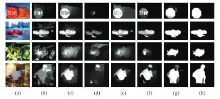
![Fig. 8: Illustrations of the superiority of the proposed WJRSR model overWSC [43]. (a) Original images; (b) WSC; (c) WJRSR; (d) Ground truth.](https://thumb-us.123doks.com/thumbv2/123dok_us/9303913.431396/6.612.107.242.56.192/illustrations-superiority-proposed-overwsc-original-images-wjrsr-ground.webp)