Short Term Scheduling of Combined Cycle Units Using Mixed Integer Linear Programming Solution

Short-Term Scheduling of Combined Cycle Units Using

Mixed Integer Linear Programming Solution

Juan Alemany1, Diego Moitre1, Herminio Pinto2, Fernando Magnago1,2

1_{Department of Electrical & Electronic Engineering, National University of Rio Cuarto, Rio Cuarto, Argentina} 2_{Nexant Inc., Chandler, USA}

Email: [email protected]

Received January 12, 2013; revised February 15, 2013; accepted February 28, 2013

ABSTRACT

Combined cycle plants (CCs) are broadly used all over the world. The inclusion of CCs into the optimal resource sche- duling causes difficulties because they can be operated in different operating configuration modes based on the number of combustion and steam turbines. In this paper a model CCs based on a mixed integer linear programming approach to be included into an optimal short term resource optimization problem is presented. The proposed method allows mod- eling of CCs in different modes of operation taking into account the non convex operating costs for the different com- bined cycle mode of operation.

Keywords: Combined Cycle Plants; Unit Commitment; Mixed Integer Linear Programming

1. Introduction

The gas-turbine combined cycle plant has been used ex- tensively in power generation, representing the great ma- jority of new generating unit installations across the globe. Combined cycle (CC) technology is now well established, becoming one of the most effective energy conversion technology at present [1,2].

The progress on CC generation technology allowed improving their thermal efficiency up to 50% approxi- matelly.

In addition, CCs present other advantages such as bet- ter environmental performance, reducing greenhouse gases, short construction lead time and low capital cost to power ratio. Moreover, the price of natural gas, which is the pri- mary fuel used for combined cycle plants, dropped.

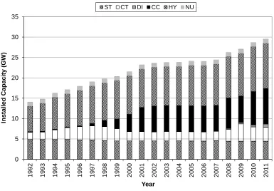
As an example of CCs use evolution, Figure 1 shows

the generation growth in Argentina since 1992 [3]. From the figure it can be seen the significant increase on the use of combined cycle plants.

Despite of their benefits, the utilization of CCs created new challenges. One of these challenges is the inclusion of combined cycle plants into the unit commitment prob- lem (UC). Modeling of CCs for UC studies is quite dif- ficult due to the tight iteraction between the gas turbine and the steam turbine generating units. These units have different operating modes; each of the operating modes has parameters such as limits or incremental heat rate that can differ considerably from each other depending on which mode is operating at the time. Therefore, the

problem needs to be expanded to determine which oper- ating mode the combined cycle units have to be in opera- tion at each time.

Several researches have been conducted to include de- tailed CC model into the UC related problems. A flexible modeling approach in order to take the multiple possible configurations into account is described in [4]. The model is based on a single unit dynamic approach that can be incorporated into a Lagrange Relaxation unit commit- ment algorithm.

Reference [5] considers the inclusion of combined cy- cle plants into an optimal short-term resource optimiza- tion. The short-term resource scheduling is realized through an Augmented Lagrange Relaxation technique. The op- timal commitment of combined cycle plants is obtained by applying a dynamic programming algorithm for a pre- viously defined combined cycle plant state space.

In [6] a method for establishing the state space dia- gram of combined cycle units for applying dynamic pro- gramming and Lagrange Relaxation to the security con- strained short-term scheduling problem is presented. Sev- eral studies verify the advantages of combined cycle units in competitive electricity markets.

0 5 10 15 20 25 30 35

1992 1993 1994 1995 1996 1997 1998 1999 2000 2001 2002 2003 2004 2005 2006 2007 2008 2009 2010 2011

Installed Capacity

(GW)

Year

ST CT DI CC HY NU

Figure 1. Evolution of electricity generation in Argentina.

Recently, advances on mixed integer programing tech- niques (MIP) allow applying this technique to very large- scale, time-varying, non-convex, mixed-integer modeling and optimization, such as unit commitment problems.

A mixed integer programing approach that allows a rigorous modeling to obtain the optimal response of ther- mal unit to an electricity spot market is proposed in [8].

An extension of this work is presented in [9] where a MIP formulation for the unit commitment problem of thermal units that allows modeling of non-convex oper- ating costs and exponential start up costs is developed.

Furthermore, a MIP solution for solving the PJM unit commitment problem is described in [10]. The paper ex- plains many of the inherent problems associated with MIP solutions and illustrates how these issues were dealt with to provide a fast, accurate, and robust MIP solution.

The first formulation of a combined cycle unit model using MIP is presented in [11] where a detailed formula- tion of a price-based unit commitment (PBUC) problem based on the MIP method is developed. The PBUC solu- tion by utilizing MIP is compared with that of Lagrange Relaxation method. As another alternative, a simplified combined-cycled unit model to solve the related mixed integer linear programming-based UC problem is shown in [12]. Although the model is simple, presents the dis- advantage of loosing solution accuracy.

Another alternative approach that model combustion turbines and steam turbines individually is presented in [13]. They applied the MIP method to solve the UC pro- blem, where the output dispatch for CC plants is set for

individual gas turbine and steam turbine generating units. According to what has been said above, it is evident that CC has acquired great relevance, particularly the de- velopment of models used for UC problems.

The aim of this paper is to develop a general and ac- curate CC model purposely designed with the idea that it could be easily included into any optimal short-term re- source optimization problem based on a mixed integer linear programing approach. The proposed model, which has taken into account studies previously done by differ- ent researchers, includes non-convex cost curves and ex- ponential start up cost curves for each operational CC mode, keeping the number of constraints to the minimum.

The paper is organized as follows; first the combined cycle model based on different modes of operation is pre- sented, then the unit commitment problem formulation based on mixed integer linear programming approach in- cluding CC units is described. After that, a numerical ex- ample is given, finally presents the most important con- clusions of the paper.

2. Combined Cycle Units

Typically, a combined cycle unit comprises of several combustion turbines (CT) and several steam turbines (ST), the waste heat from the CTs is used to produce the steam to generate additional power using STs, and this process enhances the efficiency of electricity generation.

known as modes. Each configuration is determined based on a possible combination of CTs and STs, having a de- termined generating region and an incremental heat rate curve. Configurations or modes with STs are more effi- cients; however, since the modes are restricted due to the generation region may not be more efficient for a par- ticular load and a particular simulation period.

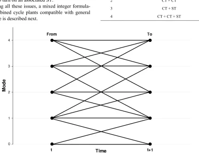
As an illustration, considering a combined cycle unit with two CTs and one STs, the related possible configu- rations are shown in Table 1, the state space is shown in Figure 2. This four mode example is used to illustrate

the problem without losing generality and can be ex- tended for any CT + ST configuration.

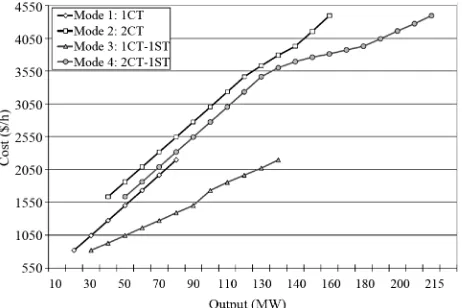
Figure 3 and Table 2 show typical incremental heat

rate curves and generation regions for this particular com- bined cycle unit. Some of the incremental heat rate cur- ves are not monotonically increasing with generation or are monotonically increasing but not convex. Therefore, if this particular condition is not considered during the optimization, the algorithm may fail to find the minimum solution.

In addition, combined cycle units have other constraints such as transition between modes and minimum time on and off for each of the modes. Furthermore, there are modes that, for a particular period, can not be eligible, for example, a CT may need to be in service for several hours prior to turn on an associated ST.

Considering all these issues, a mixed integer formula- tion for combined cycle plants compatible with general MIP software is described next.

3. MIP Algoritm

3.1. List of Symbols

t: Index for simulation hours.

b: Index for cost curve segments.

n: Index for startup cost curve.

cc: Index for combined cycle units.

m: Index for combined cycle modes.

T: Total number of simulation hours.

G: Total number of thermal units.

B: Total number of segments for production cost curve.

N: Total number of startup cost curve steps.

CC: Total number of combined cycle units.

M: Total number of combined cycle modes.

Cpg,t: Production cost for unit g at hour t [$/h]. Cpm,t: Production cost for mode m at hour t [$/h]. Cupg,t: Startup cost for unit g at hour t [$]. Cupm,t: Startup cost for mode m at hour t [$]. pg,t: Active generation for unit g at hour t [MW]. pm,t: Active generation for mode m at hour t [MW].

Table 1. Combined cycle mode example.

Mode Configuration

0 CC out of service (mode off)

1 CT

2 CT + CT

3 CT + ST

4 CT + CT + ST

Figure 3. Combined cycle modes incremental heat rate curves.

Table 2. CCs modes incremental heat rate.

Mode 1 Mode 2 Mode 3 Mode 4

MW $/h MW $/h MW $/h MW $/h

20 818 40 1636 30 818 50 1636 30 1044 60 2088 50 1044 70 2088 40 1272 80 2544 70 1272 90 2544 50 1501 100 3002 90 1501 110 3002 60 1731 120 3462 100 1731 130 3462 70 1963 140 3926 120 1963 180 3926 80 2196 160 4393 135 2196 215 4393

rg,t: Active reserve contribution of unit g, hour t [MW]. rm,t: Active reserve contribution of mode m, hour t

[MW].

δb,m,t: Active generation for segment b, mode m, hour t

[MW].

off ,

hm t

dvm,t: Slack variable for the discretization of the startup

cost function of mode m, hour t.

: Counter of hours off for mode m, hour t.

ug,t: Binary state variable for unit g, hour t. um,t: Binary state variable for mode m, hour t. sm,t: Startup variable for mode m, hour t. zm,t: Shutdown variable for mode m, hour t.

jb,m,t: Activation variable for segment b, mode m, hour t.

wn,m,t: Binary variable which activates the step n of the

stepwise startup cost of mode m at hour t.

ym,t: Startup variable for transitions to mode m, hour t. Dt: System demand at time t [MW].

Rt: System spinning reserve requirement at time t

[MW].

cm: Fixed cost for mode m [$/h].

Fb,m: Slope for segment b, mode m [$/MWh]. m

P : Maximum capacity for mode m [MW].

Pm: Minimum capacity for mode m [MW]. Pb,m: Upper limit for segment b, mode m [MW]. Kn,m: Cost for startup cost step n, mode m [$/h].

STHm: Maximum number of hours that mode m can be

off [h].

MUm: Minimum up time for mode m [h]. MDm: Minimum down time for mode m [h].

off

T

on

T





, _{1 1} min T G

m : Number of hours mode m has been off at t = 0

[h].

m : Number of hours mode m has been on at t = 0

[h].

3.2. Problem Formulation

The unit commitment problem (UC) can be formulated as a minimization problem which main objective is to determine the generation dispatch to supply the demand and reserve requirements at minimum cost over a period of time. Mathematically can be represented as follow:

g t g t u p t g  Cp Cup





t g t g t

g

G

t t g t

g

D U p

R D r

  Subject to:     





m t m m t b m b m t

b

Cp c u F 



 



(1)

Combined cycle plants can be included into the gen- eral UC formulation by modifying the cost function and adding new constraints. The changes needed for the two components of the objective function represented by Equation (1), are described below.

3.3. Production Cost

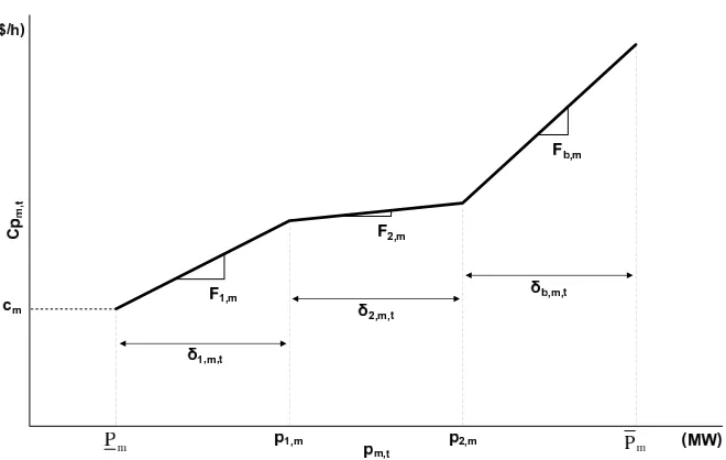
Considering the incremental cost function represented by the piecewise function of Figure 4, the production cost

function for each mode m at a simulation period t, can be formulated as: (2) Subject to: , , , , 1 B

m t m m t b m t

b

p P u 



 



For all the segments inside the curve the constraints are:









, 1, , , , ,

, , , 1, 1, , b m b m b m t b m t

b m t b m b m b m t

P P j

P P j

 



 

 

  (4)

For each mode, MW capacity restrictions apply:

, ,

m m t m t

P u p (5)

, ,

m m t m t

Figure 4. Piece wise incremental cost curve per mode.

Finally, the following restrictions related to the MW per segment, and the binary conditions of the index re- spectively are:

 

, , 0, , , 0,1

b m t jb m t

  

off

h

off off , , 1 1 m t m t

h h  





,  THm1 um t, hm t, 1 1





  

0



off

m Tm T

, , ,

1 N

m t n m n m

n

Cup K w







 

,, , , 0,1

m t wn m t

 

1

off

, , , , 1

1 N

m t n m t m t

n

dv nw h 







(7)

3.4. Startup Costs

For the startup cost model, the transition cost not only from the off state but between modes needs to be consid- ered. Figure 5 shows a typical exponential start up cost

function and the discrete representation.

First, the counter _{ m t,} that takes into account the hours that the mode m has been off is represented and formulated as follow:

(8)

off m t

h S (9)

off ,

m t m

h STH off (10) , m t h STH (11) (12) Then, based on the discretized approximation, a mathe- matical formulation for the start up cost is included per mode m and per simulation period t:

(13)

Subject to:

, , 1 N

n m t n

w y





The constraints that relate the slack variable dv(m,t) with

the start up transition binary variable y(m,t) and the startup

segment activation w(n,m,t) are:

(15)





, , , , 1 , , , ,

m t m N m t m t m t N m t dv STH w y  dv Nw

, , ,

mt t mf t mt t mf FR mt TO

y z s

 

 

(16)

These constraints are related to the logical variables as follow:





, , ,

mt t mf t mt t mf FR

y z s



 

(17)



, , 1 , ,

m t mt t m t m t u u  s z

, , 1

m t m t

s z

(19)

 

, , 0, , , , , ,, , 0,1 m t m t m t m t m t m t

s u u s z y

(20)

  





, _{1 1 1}

min T G CC

(21)

Then, the formulation explained in Subsection 3.1, can be reformulated to include combined cycle plants:

g t g t m t m y

u p t g cc

Cp Cup Cp Cup

           

 











1 1 1

0

G CC M

t g t g t m t m t

g cc m

D u p u p

   (22) Subject to:  



 

1 1 1

0

G CC M

t t g t m t

g cc m

R D r r

  

(23)







 



Figure 5. Exponential startup cost discretization.

3.5. Configuration Status

, ,

1

m t

m l m t l t MU

s u

  





, ,

1 1 m

t

m l m t l t MD

z u

  

 



off

, 0

0 m

T

m l l

u







on

, 0

1 0

m T

m l l

u



 



selected:

, 1

1 M

m t m

u







, 1 , mf t mt t u  u



, mf

mt t mt NFS

u u





(25)

3.6. Mode Transition

The restriction for the transition between mode “from” mf

and mode “to” mt can be represented as follow:

mt mf NFS

, 1

mf t 

(26)

(27)

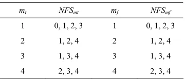
Table 3 illustrates an example for the definition of set NFSm for the 2CT-1ST case. This set is defined based on

the state space transition diagram of Figure 2.

3.7. Minimum On/Off Conditions

The modes also have restrictions due to the minimum time on and minimum time off that the generator needs to remain before the transition to another mode, these re- strictions can be formulated as:

Table 3. Transition mode variables.

mt NFSmt mf NFSmf

1 0, 1, 2, 3 1 0, 1, 2, 3

2 1, 2, 4 2 1, 2, 4

3 1, 3, 4 3 1, 3, 4

4 2, 3, 4 4 2, 3, 4

(28)

(29)

For the initial period, the number of periods the mode is on or off need to be considered:

(30)

(31)

Based on the general UC problem formulation, it was modified to include the combined cycle model into the MIP formulation, next section discusses the results con- sidering a typical power system and the addition of com- bined cycle modeled as explained in this section.

4. Numerical Results

Numerical results obtained by the proposed solution mo- del are shown in this section.

The MIP problem is solved using GAMS, and the op- timization engine selected is CPLEX 12.0. Tables 4 and 5 illustrate the CPLEX option setup.

Table 4. CPLEX options.

CPLEX option Value Description

Relative tol. 0 Force an optimal solution search

Backtracking tol. 0 Best-bound search

MIP tactic emphasize 1 Feasibility over optimality

Objective upper bound System dependant Based on a dispatch with all units in service

Objective lower bound System dependant Based on a dispatch with an heuristic priority order without reserve requirements

startup costs and minimum on/off times.

Priorities 1 Activate the use of priorities for branching

Branching rule 1 Branch on variables with maximum infeasibility

Table 5. Integer variable priorities.

Level 1 um,t

Level 2 sm,t ym,t zm,t

Level 3 jb,m,t wn,m,t dvm,t hm toff,

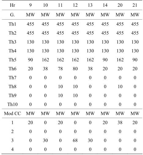
teristics are modified in order to model them as a com- bined cycle model. This allows to study the differences between a typical CC modeled as an equivalent thermal plant and modeled taking into consideration the different modes of operation. Table 6 shows the commitment re-

sults for one day simulation period, the 2CTs and 1ST are based on units 6, 7, and 8 respectively. The Table il- lustrates the dispatch for some of the simulation hours.

Table 7 illustrates the cost differences of both cases,

modelling the generator as an equivalent thermal plant or modeling the generator using the proposed combined cy- cle model. The simulations are performed for two differ- ent time horizons, in addition it shows the total simula- tion time for both models.

Then, a 20 generating system is built by duplicating the original system following the same pattern, the re- sults for this system are shown in Table 8.

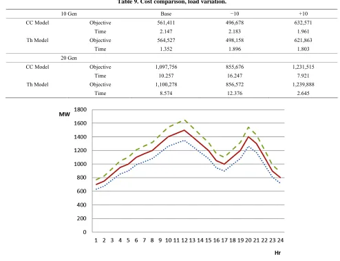
In addition, the calculations and comparisons are re- peated for different load profiles, Table 9 shows the re-

sults for a 24 h simulation period for both systems, chang- ing the base load by 10%, Figure 6 illustrates the load

profile used during the simulations.

Figure 7 shows the matrix structure of this formula-

tion applied to the 10 generation unit system, from where it can be seen the sparse structure of the matrix. For this system, after the presolve stage, the MIP array size is 144 columns and 292 rows, having 2% of nonzero elements.

The development approach gives optimal, mutually exclusive commitment of the combined cycle plant con- figurations. Results illustrate the impact of explicitly model of combined cycle units on minimizing the cost of supplying the load. The additional computer time re- quired to schedule a combined cycle unit with multiple configurations depends on the number of configurations, the number of transitions, the minumum up times, the transition times and the load profile.

Table 6. Commitment MW including a CC.

Hr 9 10 11 12 13 14 20 21

G. MW MW MW MW MW MW MW MW

Th1 455 455 455 455 455 455 455 455

Th2 455 455 455 455 455 455 455 455

Th3 130 130 130 130 130 130 130 130

Th4 130 130 130 130 130 130 130 130

Th5 90 162 162 162 162 90 162 90

Th6 20 38 78 80 38 20 20 20

Th7 0 0 0 0 0 0 0 0

Th8 0 0 10 10 0 0 10 0

Th9 0 0 10 10 0 0 0 0

Th10 0 0 0 0 0 0 0 0

Mod CC MW MW MW MW MW MW MW MW

1 20 0 20 0 0 20 38 20

2 0 0 0 0 0 0 0 0

3 0 30 0 68 30 0 0 0

4 0 0 0 0 0 0 0 0

5. Conclusion

Table 7. Cost comparison 10 Gen system.

CC Model 24 h Th Model 24 h CC Model 74 h Th Model 74 h

Model Variables 5395 5395 16,195 16,195

Statistic Equations 9306 9306 28,206 28,206

Discrete Vars 3594 3498 10,794 10,498

Non Zero Elements 34,313 34,313 104,613 104,613

MIP Objective 561,411 564,527 1,680,808 1,688,410

Solution Time 2.147 1.352 8.261 5.488

Table 8. Cost comparison 20 Gen System.

CC Model 24 h Th Model 24 h CC Model 74 h Th Model 74 h

Model Variables 10,739 10,739 32,239 2239

Statistic Equations 18,494 18,494 56,044 56,044

Discrete Vars 7188 6996 21,588 20,996

Non Zero Elements 68,633 68,633 209,233 209,233

MIP Objective 1,097,756 1,100,278 3,240,969 3,253,183

Solution Time 10.257 8.574 100.858 55.145

Table 9. Cost comparison, load variation.

10 Gen Base −10 +10

CC Model Objective 561,411 496,678 632,571

Time 2.147 2.183 1.961

Th Model Objective 564,527 498,158 621,863

Time 1.352 1.896 1.803

20 Gen

CC Model Objective 1,097,756 855,676 1,231,515

Time 10.257 16.247 7.921

Th Model Objective 1,100,278 856,572 1,239,888

Time 8.574 12.376 2.645

Figure 7. MIP matrix structure.

incorporation of feasible and non convex constraints which are present in this type of studies and very difficult to solve.

REFERENCES

[1] H. Rudnick and J. Zolezzi, “Electric Sector Deregulation and Restructuring in Latin America: Lessons to Be Learn and Possible Waysforward,” IEEE ProceedingsGenera- tion, TransmissionandDistribution, Vol. 148, No. 2, 2001, pp. 180-184. doi:10.1049/ip-gtd:20010230

[2] E. Battisti, G. Casolino, F. Rossi and M. Russo, “Eco- nomical Considerations about Combined Cycle Power Plant Control in Deregulated Markets,” InternationalJour- nalofElectricalPowerandEnergySystems, Vol. 28, No. 4, 2006, pp. 284-192. doi:10.1016/j.ijepes.2005.12.003 [3] CAMMESA, “Operational Data,” 2011.

http://www.cammesa.com

[4] A. Cohen and G. Ostrowski, “Scheduling Units with Multiple Operating Modes in Unit Commitment,” IEEE TransactionsonPowerSystems, Vol. 11, No. 1, 1996, pp. 497-503. doi:10.1109/59.486139

[5] Bjelogrlic, “Inclusion of Combined Cycle Plants into Optimal Resource Scheduling,” IEEE Proceedings of PESGeneral Meeting, San Francisco, 12-16 June 2000,

pp. 189-194.

[6] B. Lu and M. Shahidehpour, “Short-Term Scheduling of Combined Cycle Units,” IEEE Transactions on Power Systems, Vol. 19, No. 3, 2000, pp. 1616-1625.

[7] F. Gao and G. B. Sheble, “Stochastic Optimization Tech- niques for Economic Dispatch with Combined Cycle Units,” Proceedings of 9thInternational Conference on ProbabilisticMethods Applied toPower System, Stock- holm, June 2006, pp. 1022-1034.

[8] J. Arroyo and A. Conejo, “Optimal Response of a Ther- mal Unit to an Electricity Spot Market,” IEEETransac- tionsonPowerSystems, Vol. 15, No. 3, 2000, pp. 1098- 1104. doi:10.1109/59.871739

[9] M. Carrión and J. Arroyo, “A Computationally Efficient Mixed-IntegerLinear Formulation for the Thermal Unit- Commitment Problem,” IEEE Transactions on Power Systems, Vol. 21, No. 3, 2006, pp. 1371-1378.

doi:10.1109/TPWRS.2006.876672

[10] D. Streiffert, R. Philbrick and A. Ott, “A Mixed Integer Programming Solution for Market Clearing and Reliabil- ity Analysis,” IEEEProceedingsofPESGeneralMeeting, San Francisco, 12-16 June 2005, pp. 2724-2731.

tems, Vol. 20, No. 4, 2005, pp. 2015-2025. doi:10.1109/TPWRS.2005.857391

[12] G. W. Chang, G. S. Chuang and T. K. Lu, “A Simplified Combined-Cycle Unit Model for Mixed Integer Linear Programming-Based Unit Commitment,” IEEEProceed- ingsofPESGeneralMeeting, Vancouver, 6-7 July 2008, pp. 1-6.

[13] C. Liu, S. Li and M. Firuzabad, “Component and Mode

Models for the Short Term Scheduling of Combined Cy- cle Units,” IEEETransactionsonPowerSystems, Vol. 24, No. 2, 2009, pp. 976-990.

doi:10.1109/TPWRS.2009.2016501