Munich Personal RePEc Archive
Model uncertainty in matrix exponential
spatial growth regression models
Piribauer, Philipp and Fischer, Manfred M.
Vienna University of Economics and Business, Vienna University of
Economics and Business
12 June 2014
Online at
https://mpra.ub.uni-muenchen.de/77548/
Model uncertainty in matrix exponential spatial growth
regression models
Philipp Piribauer and Manfred M. Fischer
Institute for Economic Geography & GI Science
Vienna University of Economics and Business
Vienna, Austria
Correspondence: Philipp Piribauer, Vienna University of Economics and Business
e-mail: [email protected]
Abstract. This paper considers the most important aspects of model uncertainty for spatial regression
models, namely the appropriate spatial weight matrix to be employed and the appropriate explanatory
vari-ables. We focus on the spatial Durbin model (SDM) specification in this study that nests most models used
in the regional growth literature, and develop a simple Bayesian model averaging approach that provides a
unified and formal treatment of these aspects of model uncertainty for SDM growth models. The approach
expands on the work by LeSage and Fischer (2008) by reducing the computational costs through the use
of Bayesian information criterion model weights and a matrix exponential specification of the SDM model.
The spatial Durbin matrix exponential model has theoretical and computational advantages over the spatial
autoregressive specification due to the ease of inversion, differentiation and integration of the matrix
expo-nential. In particular, the matrix exponential has a simple matrix determinant which vanishes for the case of
a spatial weight matrix with a trace of zero (LeSage and Pace 2007). This allows for a larger domain of spatial
growth regression models to be analysed with this approach, including models based on different classes of
spatial weight matrices. The working of the approach is illustrated for the case of 32 potential determinants
and three classes of spatial weight matrices (contiguity-based,k-nearest neighbor and distance-based spatial
weight matrices), using a dataset of income per capita growth for 273 European regions.
Introduction
This paper considers model uncertainty associated with the selection of explanatory variables X and the
specification of the spatial weight matrixW in spatial growth regressions, where we often face a large number
of potential drivers of growth with only a limited number of observations. In particular, we focus on the
spatial Durbin model (SDM) specification that nests most models used in the regional growth literature:
(i) the spatial autoregressive (SAR) model that includes a spatial lag of growth rates from related regions,
but excludes these regions’ characteristics; (ii) the spatial error model specification in situations where
there are no omitted variables that exhibit correlation with included variables; (iii) the spatially lagged
X growth regression model (SLX) that assumes independence between regional growth rates, but includes
characteristics from related regions in the form of explanatory variablesW X; and (iv) the non-spatial linear
growth regression model (LeSage and Fischer 2008).
A natural solution to the problem of model uncertainty, supported by formal probabilistic reasoning, is the
use of Bayesian model averaging (BMA) which assigns probabilities on the model space and deals with model
uncertainty by mixing over models, using the posterior model probabilities as weights (Hoeting et al. 1999).
Fern´andez et al. (2001b) introduced the use of BMA in non-spatial least squares growth regressions with
uncertainty in the choice of regressors.1 Often the posterior probability is widely spread among many models
which strongly supports using BMA rather than choosing a single model.2 Evidence of superior predictive
performance of BMA can be found, for example, in Fern´andez et al. (2001a), and Raftery et al. (1997). Work
by Fern´andez et al. (2001a,b) considers cases where the number of potential models is sufficiently large that
calculation of posterior probabilities for all models is difficult or infeasible. But the Markov chain Monte
Carlo model composition methodology, known asM C3, proposed by Madigan and York (1995), allows for a simple treatment of potentially very large model spaces.
LeSage and Parent (2007) extended theM C3approach to the case of spatial Durbin models that contain
alternative explanatory variables conditional on a single fixed spatial weight matrix. Since the spatial
weight matrix is the hallmark of spatial growth regressions that distinguishes these from non-spatial growth
regressions, LeSage and Fischer (2008) extended this approach that can be used to increase or decrease the
number of nearest neighbors in the spatial weight matrix.3
With these authors we share the ambition to develop a Bayesian model averaging approach that
simulta-neously specifies the spatial weight or connectivity structure assigned to regions that form the observational
basis of spatial data samples, and the explanatory variables to be included in SDM growth models. But there
are a number of notable differences. From a technical point of view, LeSage and Fischer (2008) propose the
use of numerical integration techniques to obtain posterior model probabilities for model specifications with
different k-nearest spatial weight matrices. More precisely, the log-marginal likelihood for a given model
weight matrix. The posterior model probabilities are then used to obtain Bayesian model-averaged estimates.
The computational cost of this procedure makes it an impractical choice for large datasets such as these
usually considered in spatial growth empirics.
This paper expands upon this previous work of model averaging for spatial regression models by reducing
the method’s computational costs through the use of weights based on the Bayesian information criterion
(BIC) on the one side and the matrix exponential specification of the SDM on the other. This allows for a
larger domain of spatial growth regression models to be analyzed with this technique, for example, not only
those based on k-nearest neighbor spatial weight matrices as in the study by LeSage and Fischer (2008),
but also on any other type of weight matrices such as distance-based spatial weight matrices with critical
distances and the contiguity-based matrices.
We employ the matrix exponential spatial specification (MESS) of the SDM that replaces the geometric
decay by an exponential decay of spatial externalities over space. LeSage and Pace (2007) have shown that
matrix exponential spatial specifications can produce estimates and inferences similar to those from
conven-tional spatial autoregressive models, but have analytical and computaconven-tional advantages. In particular, they
simplify the log-likelihood allowing a closed form solution to the problem of maximum likelihood
estima-tion. Hence, matrix exponential spatial specifications, where the log-determinant vanishes, greatly alleviates
Markov chain Monte Carlo computations.
Model averaging is based on Bayesian information criterion (BIC) weights. Note that the posterior
model weights equal the prior model weights times the (exponentiated) Bayesian information criterion,
developed by Schwarz (1978). The BIC weights depend on the likelihood, but penalize relatively large
models through a penalty term. The implied preference for more parsimonious models addresses collinearity
among the explanatory variables. Explanatory variables that are very similar explain less of the variaton of
the dependent variable which implies less weight on such models. BIC posterior model weights have been
widely used in the literature, and provide a reasonable approximation to proper Bayesian model weights and
are moreover consistent in large samples (Doppelhofer and Weeks 2009).
It is important to note that we distinguish the terms Bayesian model comparison and Bayesian model
averaging in the following sense. Bayesian model comparison methods produce posterior model probabilities.
Bayesian model averaging uses these posterior model probabilities (produced by the comparison methods)
to weight alternative models, producing (model averaged) estimates and inferences. Some of the model
averaging literature is sloppy making a clear destinction here (see, for example, Hoeting et al. 1999). With
this clarification in mind, it appears worth noting that the study by Han and Lee (2013) deals with Bayesian
comparison in the context of three different spatial econometric models, one being a local spillover spatial
Durbin error model specification with finite distributed lags and exogenous variables, and the other a global
spillover SAR and its MESS counterpart. Model averaging, however, is outside the scope of their study.
specification of the SDM growth model, followed by an outline of the Bayesian model averaging approach
that uses a BIC approximation to the marginal likelihood for the models of interest along with a M C3
method to reduce the computational burden. The next section summarizes simulation results to investigate
the performance of our BMA approach (in terms of computational time) compared to alternative approaches
involving the computation of Bayesian marginal likelihoods that do not have closed form solutions. The
paper continues to illustrate our methodology for the case of 32 potential determinants and three classes of
spatial weight matrices (contiguity-based, k-nearest neighbor and distance-based spatial weight matrices),
using a dataset of income per capita growth for 273 European regions. We conclude with a summary and
evaluation of our results in the final section.
Matrix exponential spatial growth models
We consider cross-sectional spatial growth regression models where the dependent variable undergoes a linear
transformation as in Eq. (1):
Sy=β0ιN +Xβ+W Xγ+ε. (1)
y is anN ×1 vector of spatial observations on the dependent variable representing growth rates. X is an
N×Qmatrix of observations on theQindependent variables representing growth determinants. Each of these observations on the dependent and explanatory variables comes from regions in space. TheN-element vector
εis distributed asN(0,INσ2). βis aQ×1 vector of parameters associated with the explanatory variables, ιN is a vector of ones andβ0is the associated intercept parameter. The matrixW is anN×Nspatial weight
matrix that contains non-zero elements [W]ij if observationsjandiare neighboring regions (i, j= 1, . . . , N)
and zero otherwise. Characteristically, the matrixW is row-stochastic, so that theN×Qspatial lag matrix W X contains values constructed from an average of neighboring regions. The Q×1 parameter vectorγ measures the marginal impact of the explanatory variables from neighboring observations (regions) on the
dependent variabley.
S is anN-by-N non-singular matrix of constants that may depend on an unknown real scalar parameter
α. We focus on the transformationS used to model spatial dependence among the (regional) elements of the vectory. A prominent member of the family of spatial growth regression models given by Eq. (1) is the
conventional spatial Durbin model that arises when settingS = (IN −ρW), where ρis a scalar parameter reflecting the magnitude of spatial dependence.
The focus on this paper is on the matrix exponential as a specification forS defined in Eq. (2):
S(α) = exp(αW) =
∞
X
t=0
αt t!W
t
= IN +αW +α
2
2!W
2
+α
3
3!W
3
whereαis a real scalar parameter with−∞< α <∞. S is a linear combination of row-stochastic matrices and hence is proportional to a stochastic matrix, since products of stochastic matrices are
row-stochastic. The parameter αplays the role of ρin the conventional SDM capturing the extent of spatial dependence.
The matrix exponential spatial specification (MESS), introduced by LeSage and Pace (2007), replaces
the conventional geometric decay of influence from higher-order neighboring relations by the spatial
autrore-gressive process in conventional spatial Durbin model relationships with an exponential pattern of decay
in influence from higher-order neighboring relationships. Spatial growth regression models of type (1) with
a matrix exponential specification of S may be termed spatial Durbin matrix exponential models. For
implementation purposes, we truncate the infinite expansion shown in Eq. (2) to R terms creating an
approximation toS= exp(αW).
LeSage and Pace (2007, 2009) discussed several of the salient properties of MESS models, some of which
may be enumerated as follows: First,S(α) is non-singular (Property1). Second,S(α)−1=
exp(αW)−1
=
exp(−αW) (Property 2) and third, |exp(αW)| = exp
tr(αW)
(Property 3). Property 1 guarantees a
positive definite covariance matrix and thus avoids the need to restrict the parameter space, or to carry
out tests for positive definiteness during parameter estimation. Property 2 leads to a simple mathematical
inversion of the matrix exponential. Property 3 implies that the log-likelihood of the MESS model does not
contain a troublesome log-determinant of anN ×N matrix unlike for the case of the conventional spatial Durbin model. LeSage and Pace (2007) provide a closed form solution for the parameters of the MESS
model. Finally, it is worth noting that there are approximate relationsα≈log(1−ρ) orρ≈1−exp(α), and this relation betweenαandρfacilitates interpretations of parameter estimates for αallowing them to
be viewed in terms of the parameterρfrom the conventional spatial Durbin model.
The model averaging approach
We are interested in averaging over matrix exponential spatial growth regression models that differ in two
respects, namely the spatial weight matrix specification and the set of explanatory variables. With Q
potential growth determinants andJ potential spatial weight matrices, the cardinality of the model space
M is (IJ) withI = 22Q. A particular model M
ij ∈ M (i = 1, . . . , I;j = 1, . . . , J) is characterized by its parameter vector θ =hβ0 β
′
γ′
α σ2
i′
. In the Bayesian model averaging framework4, the posterior
for the parametersθ, calculated usingMij, is written as:
p(θ|Mij,D) =
f(D|θ, Mij)π(θ|Mij)
p(D|Mij) (3)
The posterior model probability p(Mij|D) propagates model uncertainty into the posterior distribution of model parameters. By Bayes’ rule,p(Mij|D) can be expressed as:
p(Mij|D) =
f(D|Mij)π(Mij)
p(D) ∝f(D|Mij)π(Mij) (4)
such that the posterior model probability (weight) of modelMij is proportional to the product of the
model-specific marginal likelihoodf(D|Mij) and the prior model probability π(Mij). Model weights can hence be obtained using the marginal (or integrated) likelihoodf(D|Mij) for each individual modelMij after eliciting a priorπ(Mij) over the model space. The marginal likelihood of modelMij is in turn given by:
f(D|Mij) =
Z
f(D|θ, Mij)π(θ|Mij) dθ. (5)
The ratio of marginal likelihoods of two different models is the Bayes factor and it is closely related to the
likelihood ratio statistic. Using the law of total probability the posterior density of the parameters for all
the candidate models under consideration is given by:
p(θ|D) = I
X
i=1
J
X
j=1
p(Mij|D)p(θ|Mij,D). (6)
Hence, the full posterior distribution of θ is an average of the posterior distributions under each of the
models, weighted by their posterior model probabilitiesp(Mij|D). When applying Bayesian model averaging according to Eq. (6), both estimation and inference come naturally together from the posterior distribution.
This posterior distribution provides inference about θ that takes full account of model uncertainty. As an
alternative measure of significance we can also compute the posterior inclusion probability (PIP) for a given
explanatory variable (spatial weight matrix). The posterior inclusion probability is calculated as the sum of
the posterior model probabilities for all models including that variable (spatial weight matrix).
While Bayesian model averaging is an intuitively attractive solution to the problem of accounting for
model uncertainty, its implementation in the context of our study is difficult because of two reasons. First,
the number of terms in Eq. (6) is enormous, rendering exhaustive summation infeasible. Second, the
integrals implicit in Eq. (6) are hard to compute. To tackle the first problem, Markov chain Monte Carlo
model composition (M C3) methods (Madigan and York 1995) can be used to directly approximate Eq. (6).
This approach eliminates the need to consider all possible models by constructing a sampler that explores
relevant parts of the very large model space.5
Let M denote the current model state of the chain, models are proposed using a neighborhood, say
nbd(M), which consists of the modelM itself along with models containing either one explanatory variable
more or one variable less thanM. We extend the notion of model neighborhood to include models that not only involve different matrices of explanatory variables but also different spatial weight matrices. Similarity
matrix similarity that consists of the cross-products of the matching elements in the two spatial weight
matrices6 such that:
G(WM,WM′)≡
N
X
i=1
N
X
j=1
[WM]ij[WM′]ij. (7)
The proposed modelM′
is compared to the current model state using the following acceptance probability:
min
"
1,p(M
′
|D)
p(M|D)
#
. (8)
GivenJ distinct (contiguity-based,k-nearest neighbor and distance-based) spatial weight matrices, we get a
J×J matrixGrepresenting the pair-wise similiarities between any two weight matrices. Row-normalization (i. e., dividing the elements by the respective row-sums) yields a matrix that describes the transition
probability vector from a particular spatial weight matrix to another. It is important to note that conditional
onWM (i. e., the spatial weight matrix in current stateM), ourM C3 algorithm simultaneously draws a
spatial weight matrix for each recursion.7
The second difficulty in implementing Bayesian model averaging is that the integrals implicit in Eq. (6)
are hard to compute. For matrix exponential spatial growth regression models, closed form integrals for the
marginal likelihood (5) are not available. We therefore use Bayesian information criterion (BIC) weights as
an approximation tof(D|Mij):
f(D|Mij)≃f(D|θˆ, Mij)N
−dij/2 (9)
where ˆθ is the maximum likelihood estimate of the parameter vector θ in model Mij, and dij denotes
the number of parameters in model Mij. Bayesian information criterion model weights have been widely
discussed in the literature (see Schwarz 1978, Kass and Wasserman 1995, Raftery 1995). When the number
of observations becomes large or rather non-informative priors are used, we may furthermore assume that
the expectation of the posterior distribution equals the maximum likelihood estimates. There exist several
approaches which make use of BIC as a means to approximate posterior model probabilities in the empirical
growth literature. For example, Sala-i-Martin et al. (2004) advocate frequentist ordinary least squares
estimates along with BIC model weights. This approach became known as Bayesian model averaging of
classical estimates (BACE). A generalization to maximum likelihood estimates is provided by Moral-Benito
(2012). The use of information-theoretic quantities to calculate model weights is moreover extensively used in
the frequentist model averaging literature. Frequentist model averging techniques are thoroughly described
in Burnham and Anderson (2004), and Claeskens and Hjort (2008).
Model priors π(Mij) are the only quantities which remain to be chosen. Many studies use a uniform
model prior structure by assigning equal probability to the models prior seeing the data D. However, a uniform prior structure would implicitly impose a mean prior model size ofQ, since the majority of models
proposed in the literature. For example, Ley and Steel (2009) propose the use of binomial-beta priors which
uses a hyperprior on the inclusion of each regressor:
π(Mij)∝Γ(1 +ϕij)Γ(1 + 2Q−ϕij) (10)
where Γ(·) and ϕij denote the gamma function and the number of non-constant covariates in model Mij, respectively. Unlike a uniform model prior, which attaches uniform prior mass to the respective models, the
prior given in Eq. (10) is uniform over prior expected model size.
Monte Carlo experiments
Before turning to an illustrative example, we present the results of Monte Carlo experiments to investigate the
performance of the approach outlined above in comparison to two alternative approaches, namely Bayesian
model averaging of spatial Durbin models put forward by LeSage and Fischer (2008), and Bayesian model
averaging of spatial Durbin matrix exponential model specifications as proposed by LeSage and Pace (2007).
The latter approaches involve the computation of Bayesian marginal likelihoods which do not have closed
form solutions. The evaluation of the marginal posteriors forρandαrequires numerical integration over a
fine grid of the respective parameter space.
For Bayesian model averaging of conventional spatial Durbin models we define the prior for ρto follow
a uniform distribution π(ρ) ∼ U(−1,1). To increase computational speed we used the log-determinant approximation proposed by Pace and Barry (1998). For its MESS counterpart we used a normal distribution
with zero mean and a standard deviation of ten as a prior specification for α. In this setting we use
numerical integration over the interval α ∈[−3,3]. Note that both prior specifications are rather diffuse. On the slope parameters we use the well-known Bayesian risk inflation criterion (BRIC) specification for
theg-prior as proposed by Fern´andez et al. (2001a). For the parameters which are common to all models
(i. e., the parameter on the constant term β0 and σ2) non-informative priors are used (see Fern´andez
et al. 2001b, Koop 2003).
We conduct Monte Carlo experiments by drawing five potential independent variables
X =hx1 x2 · · · x5 i
using N = 273 draws from a standard normal distribution for each covariate, so
as to match the sample size of our empirical application in the next section. The experiment examined nine
cases that vary by the degree of spatial autocorrelation in the dependent variable as well as the
signal-to-noise ratio. We consider three cases of the degree of spatial autocorrelation, namelyα=−0.10 (ρ≈0.1),
α=−1.00 (ρ≈0.63), and α=−2.00 (ρ≈0.86). Data on the dependent variable are generated according to:8
y= exp(1W)(1ιN + 1.5x1+ 2x2−0.5x3+ 3W x2−2W x3−0.5W x4+ 0.25ε) (11)
the signal-to-noise ratio (SNR) equaled 0.1, 0.5, or 0.9. The N ×N spatial weight matrix is treated as fixed using a seven nearest neighbor specification based on standard uniform draws of longitude and latitude
values. The set of potential (non-constant) regressors is given byhX W X
i
, which yields a cardinality of
the model space of 210.
The data generating process in Eq. (11) is chosen such that one variable (x1) enters the equation without
its spatial lag, two variables (x2andx3) exert both lagged and non-lagged effects, one variable (x4) involves
only its spatial lag and one variable (x5) neither enters in its original nor in its spatially lagged form.
[Table 1 about here]
All computations were carried out on a computer with a 3.33 GHz processor using Windows 7 and
MATLAB version 8.1.0.604 (R2013a). The BMA approaches under consideration were carried out to produce
250 draws with the first 50 discarded to allow the M C3 algorithm to converge to a steady state. The
estimation results are reported in Table 1. They relate to averages over 1,000 simulated runs. True values used to generate the data are reported in the first column. The table reports the simulation results of
the three approaches under consideration in the columns that follow: first, the BMA approach based on
BIC weights and spatial Durbin matrix exponential model (SDMEM) specifications, then BMA based on
Bayesian posterior model probabilities (PMP) and spatial Durbin matrix exponential model specifications,
and finally BMA based on PMP and conventional spatial Durbin model (SDM) specifications.
For each approach the table reports the posterior means of the respective parameters along with
aver-aged timing results and the Bayesian information criterion (as a measure of the in-sample fit). In all cases
using different values of SNR andα, the results indicate that the approach using BIC and maximum
likeli-hood estimates of MESS outperforms both SDM and SDMEM specifications using Bayesian posteriors and
marginal likelihoods, in terms of in-sample performance as well as computational efficiency. Not surpisingly,
the conventional SDM specification yields the largest BIC. Overall, Table 1 reveals that the best in-sample
fits can be achieved for moderate degrees of spatial autocorrelation (α=−1).
The posterior mean estimates for all parameters are very close to their true values. Specifically, the
estimated parameters in the SDMEM approaches are most similar to the true values. Albeit misspecified,
conventional spatial Durbin model specifications also yield results very close to the true data generating
process, which is largely owing to the close relationship of MESS and conventional specifications of global
spillovers (see LeSage and Pace 2007). Comparing the average posterior means of SDMEM using BIC and
Bayesian posterior model probabilities shows that for large signal-to-noise ratios the BIC approach tends
to be closer to the true parameter values compared to the approach using Bayesian marginal likelihoods.
This may be due to the fact that the Bayesian framework additionally involves the use of prior information,
whereas the BIC approach relies only on information from the sampled data.
conventional spatial Durbin models. They also indicate that our approach is computationally faster than
the other existing approaches. We see a speed improvement in computation times that is attributable to the
fact that the approach strictly relies on closed form solutions and avoids the calculation of log-determinants
as a consequence of the theoretical properties of MESS models. In summary, the results indicate that our
approach using BIC weights and maximum likelihood estimates of SDMEM outperforms both other BMA
approaches in terms of in-sample performance and computational efficiency.
An applied illustration
This section serves to illustrate the working of the model averaging approach on a matrix exponential spatial
specification of the spatial Durbin growth regression for both identifying model covariates and unveiling
spatial structures in pan-European growth data.
The sample data
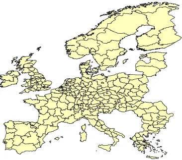
Our sample is a cross-section of 273 European regions representing 28 European countries9over the 2000-2010
period. The units of observation are the NUTS-2 regions (NUTS revision 2010).10 These regions, though
varying in size, are generally considered to be appropriate spatial units for modeling and analysis purposes.
In most cases, they are sufficiently small to capture subnational variations. But we are aware that NUTS-2
regions are formal rather than functional regions, and their delineation does not represent the boundaries of
regional growth processes very well. The sample regions include regions located in Austria (nine regions),
Belgium (11 regions), Bulgaria (six regions), Czech Republic (eight regions), Denmark (five regions), Estonia
(one region), Finland (five regions), France (22 regions), Germany (38 regions), Greece (13 regions), Hungary
(seven regions), Italy (21 regions), Latvia (one region), Lithuania (one region), Luxembourg (one region),
Netherlands (12 regions), Norway (seven regions), Poland (16 regions), Portugal (five regions), Republic of
Ireland (two regions), Romania (eight regions), Slovakia (four regions), Slovenia (two regions), Spain (16
regions), Sweden (eight regions), Switzerland (seven regions) and the United Kingdom (37 regions). A map
of the regions used is depicted in Figure 1.
[Figure 1 about here]
We use gross-value added (gva), rather than gross regional product at market prices as a proxy for regional
income. The proxy is measured in accordance with the European System of Accounts (ESA) 1995. The
data for the European regions come from the Cambridge Econometrics database. The dependent variable
represents average per capita growth rates over the period 2001-2010.
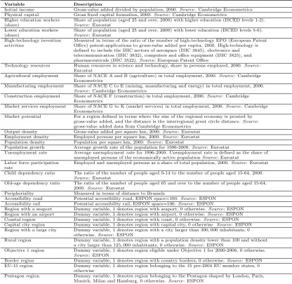
We consider a set ofQ= 32 candidate explanatory variables as well as their spatially lagged forms. To avoid
potential endogeneity problems all the variables are measured at the beginning of the sample period (that
is, 2000). The variable names and the data sources are depicted in Table 2. A very popular variable in the
regional growth regression literature is the initial level of income. Most studies include this variable and find
it to be significant. Proxies for human capital are also widely considered as a key determinant of economic
growth. We measure human capital by the skills of the workforce as given by the level of educational
attainment of the population, and distinguish between lower and higher educated workers, where high and
low education levels are defined by the ISCED (international standard classification of education) levels 1-2
and 5-6, respectively. We also included physical capital stocks constructed using the perpetual inventory
method using a depreciation rate of ten per cent and investment data for the years 1990-2000.
There is substantial empirical evidence supporting the role of high-technology firms in technological
change and economic growth. Despite the inherent difficulties in measuring the effects of technological
progress on economic growth we rely on two candidate variables that capture different aspects of the process
of innovation and technological change at the regional level. We consider the ratio of the number of
high-technology patent applications at the European Patent Office (EPO) to gross-value added per capita as a
proxy for the output of high-technology invention activities in each region. Another candidate variable, the
share of human resources employed in science and technology, represents a technology input measure. To
ac-count for the industrial mix, we also consider the shares of employment in agriculture,
mining-manufacturing-energy, construction, and market services. Harris (1954), and LeSage and Fischer (2008) argue that market
access is also important for regional income. We therefore include an index of market potential that measures
the export demand each region faces given its spatial location and that of its trading partners.
Theoretical as well as empirical studies show that the age-structure of the population might exert a
decisive effect on economic growth (see Azomahou and Mishra 2008, Boucekkine et al. 2002). We rely on
two measures to proxy the demographic structure of the regions. First, the child-dependency ratio of a
region which is defined as the number of people aged 0-14 as a ratio to the number of people aged 15-64.
Second, the old-age dependency ratio of a region which is given by the ratio between the number of people
aged 65 and over and the number of people aged 15-64. Both variables capture the burden of the economic
productive part of the population to maintain the economically dependent.
Moreover, we follow Fingleton (2001) and consider population density, employment density and output
density as candidate explanatory variables to control for urban agglomerations. Urban agglomerations are
typically equipped with larger human capital stocks as a repository of knowledge, which facilitates innovation
creation and adoption and thus accelerates technological progress and economic growth. Finally, we also
include candidate explanatory variables in the regressions with the purpose of accounting for likely differences
in the access to sea, roads, air and rail transport, and a series of dummy variables suggested by Crespo
Alternative spatial weights
In order to illustrate the ability of our approach toboth identify model covariates and unveil spatial
struc-tures present in the data, we restrict our space of potential (row-normalized) spatial weight matrices to three
different classes: (binary) Queen contiguity-based matrices, (binary) k-nearest neighbor matrices and
(bi-nary) distance-based matrices. Queen contiguity-based matrices consider regions as neighbors if they share
a common border (including cases where the common border is just a vertex). We will consider first-order
and second-order contiguity definitions for neighbors in this class. k-nearest neighbor matrices constrain
the neighbor structure to the k-nearest neighbors and thereby precluding islands and forcing each region
to have the same number of neighbors. For this class of weighting matrices, we consider k = 5, . . . ,14.
Finally, distance-based matrices are based on a distance criterion, such that two regionsiandj are defined
as neighbors when the distance between them is less than a given critical valued. Critical distance is defined
here by the first and second quintile of the entire distribution, respectively.
k-nearest neighbor and distance-based spatial weight matrices are used with three alternative distance metrics that reflect different aspects of spatial connectivity: (i) geodesic distances, (ii) road travel time
distances for cars, and (iii) drive time distances for heavy goods vehicles. LeSage and Fischer (2008) argue
that drive time measures of distance reflect economic distance which may introduce important aspects to
connectivity. The structure of the road networks, presence of mountains, rivers, landlocked areas, national
car and lorry speed limit, as well as statutory rest periods for drivers may lead to considerable differences
between geodesic and drive time distances. The travel time spatial weight matrices are based on information
on road infrastructure from the European transport network database of the Institute of Spatial Planning
in Dortmund (IRPUD) based on reference year 2005.
A comparison of alternative spatial weight matrices
An important point to note about spatial model comparison is that the performance will depend on the
strength of the spatial dependence in the sample data. LeSage and Pace (2009) illustrate this for spatial
weight matrix comparisons in the case of conventional SAR models using data generated experiments. They
show that values for the spatial dependence parameter close to zero make it difficult to distinguish between
alternative spatial weight matrices. Since the spatial dependence in our growth model is moderately strong,
withρ≈0.64, this should not present a problem here.
[Table 3 about here]
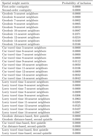
Posterior probabilities of inclusion for the 38 spatial weight matrices are shown in Table 3. We see support
for a spatial weight matrix based on 10 (probability of inclusion: 0.396) and 11 nearest neighbors
respectively. Since the average number of first-order contiguous neighbors for the European regions in our
sample is near five, and the average number of second-order contiguous neighbors is 13, this suggests a
spatial connectivity structure that extends beyond first-order contiguous regions, but not to all second-order
contiguous neighbors.
High probability matrix exponential spatial growth regression models
Running theM C3sampler for 30 million draws and discarding the first 5 million iterations produced 114,864
unique models. Note that there are 264≈1.84 1019 possible models based on alternative ways to combine
the 32 candidate explantory variables and their spatial lags, and for each of these another 38 possible spatial
weight matrices that can be used with each of these models. As a test for convergence of theM C3procedure,
we produced several runs of the sampler using different starting models which resulted in correlations between
posterior model probabilities above 0.99. In all cases, the results are nearly identical, suggesting that the
M C3 procedure is converging sufficiently.11
[Table 4 about here]
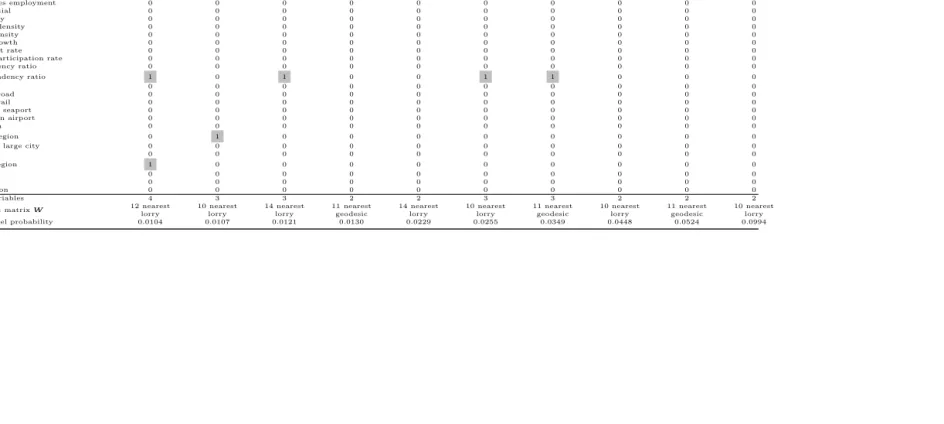
Table 4 shows the variables appearing in the ten highest posterior probability models, along with the model
probabilities. The posterior probabilities for these models are (0.0994, 0.0524, 0.0448, 0.0349, 0.0255, 0.0229,
0.0130, 0.0121, 0.0107, 0.0104) accounting for 33.9 percent of the posterior probability mass. Variables that
appear in the respective models are designated with a ’1’, and those that do not appear with a ’0’. The bottom
rows of the table show the number of variables included, the particular spatial weight matrix employed, and
the posterior model probability. Fern´andez et al. (2001b) provide details on calculations of posterior inclusion
probabilities of individual variables. We find that two of the 32 variables (initial income and lower education
workers) appear in all ten highest probability models, and two variables (capital city regions and Objective
1 regions) appear in one model and not in others. Another 27 of the 32 variables do not appear in one of
the top ten models.
Model averaged parameter and impact estimates
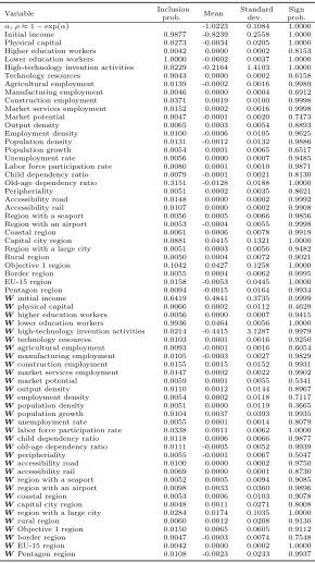
Table 5 depicts the posterior inclusion probabilities and model-averaged parameter estimates of the variables
and their spatial lags. In addition to posterior standard deviations, Table 5 also reports conditional sign
cer-tainty probabilities as another measure of the significance of variables and their spatial lags (see Sala-i-Martin
et al. 2004). Conditional sign certainty probabilities are calculated from the marginal posterior distribution
which only consists of models where the respective variable or its spatial lag is included. Conditional on the
inclusion of a variable or its spatial lag this metric measures the probability that a coefficient has the same
sign as its posterior mean.
The posterior mean (i. e., the model averaged estimate) of the spatial autocorrelation parameter ρ (ρ≈
1−exp(α)) amounts to 0.64. With a corresponding posterior standard deviation of 0.11,αis estimated very precisely. The high magnitude of the estimated spatial autocorrelation parameter stresses the importance
of accounting for spatial dependence in the observations, since it is well-known that an erroneously omitted
spatial lag in the dependent variable results in biased and inconsistent parameter estimates (LeSage and
Pace 2009).
With posterior inclusion probabilities close to unity, we identify the variable lower education attainment
and its spatial lag as well as the variable initial income as the most important growth determinants. The
posterior mean of initial income has a negative sign with a sign certainty probability of unity. Our results
thus suggest that poorer regions grow, on average, faster than richer regions – after controlling for other
factors – highlighting income convergence among the regions in the sample. Interestingly, Table 5 reveals a
positive posterior mean of the spatial lag of initial income giving rise to positive growth spillovers emanating
from the intital income of neighboring regions. Regions thus may benefit from being close to rich neighbors.
But the spatial lag of initial income receives with a probability of inclusion of 64 percent only moderate
posterior support. The negative conditional income convergence effect appears to outweight positive growth
spillovers from neighboring regions.
Both lower educational attainment measured in terms of primary and lower secondary education
repre-senting the highest degree obtained by population aged 25 and over, and its spatial lag exhibit a posterior
probability of inclusion of unity. As expected, the variable lower education workers has a negative posterior
mean. However, our results also suggest a positive posterior mean of its spatial lag. While a poorly educated
labor force hampers income growth in the same region, our results also reveal positive effects on income
growth rates to neighboring regions. Assuming that an increase in the lower educated labor force is mainly
caused by migration of workers between regions, the negative correlation between lower educated workers
and income growth results in positive spillover effects (see Olejnik 2008).
[Table 6 about here]
In Table 6 we report model averaged direct and indirect impact estimates based on the 114,864 models found
by the M C3 algorithm. From the estimates we see that the impact estimates of 30 from the 32 variables
fell within two standard deviations of zero. This leaves us with two variables from the set of candidate
explanatory variables that exerted significant total impact on growth with probabilities of inclusion above
99 percent. These variables were initial income and educational attainment measured by primary and lower
secondary education representing the highest degree obtained by population aged 25 and over. Initial income
was found to exert both a negative direct and total impact on growth. The respective spatial spillover effect,
however, was estimated very imprecisely. The educational attainment variable had a negative direct, but
share of low-educated in working age population in all other regions. Both estimates were found to be highly
significant.
In concluding we note that our approach allowed us to provide estimates and inference, which variables
from a set of 32 candidate explanatory variables exerted a significant impact on economic growth rates. Only
two of these variables (initial income and lower education) were found to exhibit a posterior probability of
inclusion close to unity. Both initial income and lower education exert a negative influence. But it is worth
noting that the direct impact of the latter variable is −0.058 and the spillover impact 0.020 revealing the total negative influence. Moreover, we see support for spatial weight matrices based on 10 and 11 nearest
neighbors where distance is measured in terms of lorry travel times and geodesic distances, respectively.
Closing remarks
This paper represents a formal Bayesian solution to the problem of uncertainty regarding the most important
aspects of model specification that arise in applied practice. The problem of model uncertainty can arise from
several sources. First, the selection of appropriate variables is a difficult issue in growth empirics and involves
a trade-off between the arbitrary selection of a small number of variables, which may imply some omitted
variables bias, and the introduction of a larger set of variables with a number of econometric problems such
as endogeneity or multicollinearity. A second source of model uncertainty arises in a spatial setting. One
also has to specify the spatial weight matrix that defines connectivity between regions. LeSage and Fischer
(2008) focus on k-nearest spatial weight matrices and accomplish this by extending the M C3 approach of
LeSage and Parent (2007) that is used to increase or decrease the number of nearest neighbors in the spatial
weight matrix. From a technical point of view, this approach uses numerical integration techniques to obtain
posterior model probabilities for model specifications based on spatial weight matrices with differing numbers
of nearest neighbors, and is thus not feasible for models based on other classes of spatial weight matrices.
Moreover, the computional costs make it impractical for larger sets of covariates.
The model averaging approach introduced in this paper overcomes these shortcomings. This is
accom-plished by using first BIC as a means to approximate marginal likelihoods, second using spatial Durbin
matrix exponential model specifications to produce a closed-form solution for maximum likelihood
estima-tion, and third by extending the notion of model neighborhood to include models that not only involve
different matrices of explanatory variables but also different spatial weight matrices.
Monte Carlo experiments demonstrated that our approach is computationally faster than other existing
approaches. The improvement in computation times is attributable to the fact that the approach strictly
relies on closed form solutions and avoids the calculation of log-determinants as a consequence of the
the-oretical properties of MESS models. Moreover, it is worth mentioning that the simulations demonstrated
conventional SDM models.
Notes
1
An alternative way (the so-called Bayesian averaging of classical estimates (BACE) approach) of dealing with the issue of variable selection in non-spatial least squares regressions is proposed in Sala-i-Martin et al. (2004). This approach is not totally Bayesian, as it is not formally derived from a prior likelihood specification, but relies on an approximation as sample size goes to infinity.
2
Other papers using BMA in the context of conventional least squares growth regressions are Masanjala and Papageorgiou (2008), Le´on-Gonz´alez and Montolio (2004), among others.
3
Note that LeSage and Fischer (2012) extended to include not only spatial, but also technological dependencies.
4
For an introduction to Bayesian model averaging, see, for example, Koop (2003).
5
For more details onM C3
sampling see Madigan and York (1995), Koop (2003) and Fern´andez et al. (2001b). Note that the sampler is only a tool to deal with the practical impossibility of exhaustive analysis ofM, by only visiting the models which
have non-negligible posterior support.
6
Note that theGindex has been applied to spatial autocorrelation by Hubert et al. (1985) and Anselin (1995), among others.
7
The validity of the concordance approach relies on the assumptions that the spatial weight matrices are row-stochastic and that the main diagonal element in each row of the resulting transition probability matrix is larger than any off-diagonal element in the same row.
8
MATLAB functions for the comparison of the three approaches are available upon request.
9
EU-27 member states plus Norway and Switzerland minus Cyprus.
10
We exlude the Spanish North African territories of Ceuta and Melilla, the Canary Islands, the Portuguese non-continental territories A¸cores and Madeira, the French D´epartements d’Outre Mer Guadeloupe, Martinique, Guyane and R´eunion. Moreover, because of data availability problems we use the NUTS revision of 2006 rather than 2010 for the Finnish regions ˆ
Aland, Etel¨a-Suomi, It¨a-Suomi, L¨ansi-Suomi and Pohjois-Suomi.
11
References
Anselin, L. (1995). ”Local indicators of spatial association – LISA.”Geographical Analysis 27(2), 93–115.
Azomahou, T., and T. Mishra (2008). ”Age dynamics and economic growth: Revisiting the nexus in a
nonparametric setting.”Economic Letters 99(1), 67–71.
Boucekkine, R., D. de la Croix, and O. Licandro (2002). ”Vintage human capital, demographic trends, and
endogenous growth.”’Journal of Economic Theory 104(2), 340–75.
Burnham, K., and D. Anderson (2004). ”Multimodel inference: Understanding AIC and BIC in model
selection.”Sociological Methods & Research 33(2), 261–304.
Claeskens, G., and N. Hjort (2008).Model selection and model averaging. Cambridge: Cambridge University
Press.
Crespo Cuaresma, J., and M. Feldkircher (2013). ”Spatial filtering, model uncertainty and the speed of
income convergence in Europe.”Journal of Applied Econometrics 28(4), 720–41.
Crespo Cuaresma, J., G. Doppelhofer, and M. Feldkircher (2014). ”The determinants of economic growth in
European regions.”Regional Studies, 48(1), 44–67.
Doppelhofer, G., and M. Weeks (2009). ”Jointness of growth determinants.”Journal of Applied Econometrics
24(2), 209–44.
Fern´andez, C., E. Ley, and M. Steel (2001b). ”Benchmark priors for Bayesian model averaging.”Journal of
Econometrics 100(2), 381–427.
Fern´andez, C., E. Ley, and M. Steel (2001a). ”Model uncertainty in cross-country growth regressions.”
Journal of Applied Econometrics 16(5), 563–76.
Fingleton, B. (2001). ”Theoretical economic geography spatial econometrics: Dynamic perspectives.”Journal
of Economic Geography 1(2), 201–25.
Han, X., and L. Lee (2013). ”Bayesian estimation and model selection for spatial Durbin error model with
finite distributed lags.”Regional Science and Urban Economics 43(5), 816–37.
Harris, C. (1954). ”The market as a factor in the localization of industry in the United States.” Annals of
the Association of American Geographers 44(4), 315–48.
Hoeting, J. A., D. Madigan, A. Raftery and C. Volinsky (1999). ”Bayesian model averaging: A tutorial.”
Hubert, L., R. Golledge, C. Constanzo, and N. Gale (1985). ”Measuring association between spatially defined
variables: An alternative procedure.”Geographical Analysis 17(1), 36–46.
Kass, R., and L. Wasserman (1995). ”A reference Bayesian test for nested hypotheses and its relationship
to the Schwarz criterion.”Journal of the American Statistical Association 90(431), 928–34.
Koop, G. (2003).Bayesian Econometrics. Chichester: John Wiley & Sons.
L´eon-Gonz´alez, R., and D. Montolio (2004). ”Growth, convergence and public investment: A Bayesian model
averaging approach.”Applied Economics 36(17), 1925–36.
LeSage, J., and M. M. Fischer (2012). ”Estimates of the impact of static and dynamic knowledge spillovers
on regional factor productivity.”International Regional Science Review 35(1), 103–27.
LeSage, J., and M. M. Fischer (2008). ”Spatial growth regressions, model specification, estimation, and
interpretation.”Spatial Economic Analysis 3(3), 275–304.
LeSage, J., and K. Pace (2009).Introduction to Spatial Econometrics. Boca Raton: CRC Press.
LeSage, J., and K. Pace (2007). ”A matrix exponential spatial specification.” Journal of Econometrics
140(1), 190–214.
LeSage, J., and O. Parent (2007). ”Bayesian model averaging for spatial econometric models.”Geographical
Analysis 39(3), 241–67.
Ley, E., and M. Steel (2009). ”On the effect of prior assumptions in Bayesian model averaging with
applica-tions to growth regression.”Journal of Applied Econometrics 24(4), 651–74.
Madigan, D., and J. York (1995). ”Bayesian graphical models for discrete data.” International Statistical
Review 63(2), 215–32.
Masanjala, W., and C. Papageorgiou (2008). ”Rough and lonely road to prosperity: A reexamination of
the sources of growth in Africa using Bayesian model averaging.” Journal of Applied Econometrics
23(5), 671–82.
Moral-Benito, E. (2012). ”Determinants of economic growth: A Bayesian panel data approach.”The Review
of Economics and Statistics 94(2), 566–79.
Olejnik, A. (2008). ”Using the spatial autoregressively distributed lag model in assessing the regional
con-vergence of per-capita income in the EU25.”Papers in Regional Science 87(3), 371–84.
Pace, K., and R. Barry (1998). ”Simulating mixed regressive spatially autoregressive estimators.”
Raftery, A. (1995). ”Bayesian model selection in social research.”Sociological Methodology 25, 111–63.
Raftery, A., D. Madigan and J. A. Hoeting (1997). ”Bayesian model averaging for linear regression models.”
Journal of the American Statistical Association 92(437), 179–91.
Sala-i-Martin, X., G. Doppelhofer, and R. I. Miller (2004). ”Determinants of long-term growth: A Bayesian
averaging of classical estimates (BACE) approach.”American Economic Review 94(4), 813–35.
Table 1 Results of the Monte Carlo experiments, averaged over 1,000 simulation runs
α=−0.10 α=−1.00 α=−2.00
BIC Weights PMP Weights BIC Weights PMP Weights BIC Weights PMP Weights SNR Variables/ True SDMEM SDMEM SDM SDMEM SDMEM SDM SDMEM SDMEM SDM
BIC Mean Mean Mean Mean Mean Mean Mean Mean Mean
x1 1.50 1.48 1.50 1.50 1.49 1.49 1.45 1.51 1.51 1.45
x2 2.00 1.98 2.01 2.01 2.00 2.00 1.99 2.03 2.02 2.18
x3 -0.50 -0.43 -0.37 -0.37 -0.49 -0.48 -0.51 -0.49 -0.49 -0.65 x4 0.00 0.00 0.00 0.00 0.00 0.00 0.00 0.00 0.00 -0.01
x5 0.00 0.01 0.00 0.00 0.00 0.00 0.00 0.00 0.00 0.00
0.10 W x1 0.00 0.04 0.02 0.03 0.02 0.01 0.10 0.00 0.00 0.98
W x2 3.00 2.95 2.99 3.05 3.10 3.04 3.41 3.13 3.07 5.18
W x3 -2.00 -1.93 -1.96 -1.99 -2.05 -2.03 -2.13 -2.05 -2.03 -2.81 W x4 -0.50 -0.33 -0.14 -0.15 -0.19 -0.19 -0.21 -0.32 -0.30 -0.44 W x5 0.00 -0.15 -0.01 -0.01 0.03 0.03 0.03 0.02 0.02 0.01
ˆ
α, ˆρ -0.09 -0.10 0.08 -0.97 -0.98 0.63 -1.97 -1.99 0.85 BIC 584.14 598.04 598.21 548.97 549.07 551.13 798.81 799.15 867.36
x1 1.50 1.48 1.48 1.48 1.49 1.49 1.45 1.51 1.51 1.45
x2 2.00 2.01 2.00 2.01 2.00 1.99 2.00 2.02 2.01 2.20
x3 -0.50 -0.50 -0.50 -0.51 -0.50 -0.50 -0.53 -0.50 -0.50 -0.66 x4 0.00 0.00 0.00 0.00 0.00 0.00 0.00 0.00 0.00 -0.02 x5 0.00 0.00 0.00 0.00 0.00 0.00 0.00 0.00 0.00 -0.01
0.50 W x1 0.00 0.00 0.00 0.00 0.01 0.00 0.13 0.02 0.01 1.18
W x2 3.00 3.17 3.11 3.16 3.06 2.99 3.46 3.12 3.05 5.38
W x3 -2.00 -2.02 -2.00 -2.02 -2.05 -2.02 -2.15 -2.11 -2.08 -2.94 W x4 -0.50 -0.19 -0.19 -0.20 -0.23 -0.23 -0.26 -0.26 -0.25 -0.44 W x5 0.00 -0.01 -0.01 -0.01 0.00 0.00 -0.01 -0.01 -0.01 -0.03
ˆ
α, ˆρ -0.07 -0.09 0.07 -0.99 -1.01 0.64 -1.98 -2.00 0.84 BIC 435.70 435.84 435.95 395.95 396.23 402.38 639.56 639.99 719.14
x1 1.50 1.50 1.50 1.49 1.49 1.49 1.45 1.50 1.50 1.47
x2 2.00 2.00 1.99 2.00 2.00 1.99 2.02 2.00 1.99 2.24
x3 -0.50 -0.51 -0.50 -0.50 -0.50 -0.50 -0.54 -0.51 -0.50 -0.68 x4 0.00 0.00 0.00 0.00 0.00 0.00 0.00 0.00 0.00 -0.03
x5 0.00 0.00 0.00 0.00 0.00 0.00 0.00 0.00 0.00 0.00
0.90 Wx1 0.00 0.02 0.00 0.01 0.00 -0.02 0.27 0.01 -0.02 1.32
W x2 3.00 3.03 2.95 2.99 3.03 2.95 3.59 3.04 2.94 5.68
W x3 -2.00 -2.02 -1.99 -2.00 -2.01 -1.98 -2.20 -2.01 -1.97 -3.07 W x4 -0.50 -0.43 -0.42 -0.43 -0.50 -0.49 -0.51 -0.50 -0.49 -0.64 W x5 0.00 0.00 0.00 -0.01 0.00 0.00 0.00 0.00 0.00 0.02
ˆ
α, ˆρ -0.09 -0.12 0.10 -0.99 -1.02 0.61 -1.99 -2.02 0.82 BIC -6.48 -6.33 -6.21 -42.17 -41.85 -25.48 201.61 202.39 385.39
Time [sec.] 0.64 96.57 87.84 0.64 95.48 87.59 0.63 96.29 87.52
SNR stands for the signal-to-noise ratio, SDMEM for the spatial Durbin matrix exponential model, and SDM for the spatial Durbin model. BIC refers to the Bayesian
Table 2 The variables used in the analysis
Variable Description
Initial income Gross-value added divided by population, 2000.Source: Cambridge Econometrics Physical capital Gross fixed capital formation, 2000.Source: Cambridge Econometrics
Higher education workers (share)
Share of population (aged 25 and over, 2000) with higher education (ISCED levels 1-2). Source: Eurostat
Lower education workers (share)
Share of population (aged 25 and over, 2000) with lower education (ISCED levels 5-6). Source: Eurostat
High-technology invention activities
Measured in terms of the ratio of the number of high-technology EPO (European Patent Office) patent-applications to gross-value added per capita, 2000. High-technology is defined to include the ISIC sectors of aerospace (ISIC 3845), electronics and telecommunication (ISIC 3832), computers and office equipment (ISIC 3825), and pharmaceuticals (ISIC 3522).Source: European Patent Office
Technology resources Human resources in science and technology, share in persons employed, 2000.Source: Eurostat
Agricultural employment Share of NACE A and B (agriculture) in total employment, 2000.Source: Cambridge Econometrics
Manufacturing employment Share of NACE C to E (mining, manufacturing and energy) in total employment, 2000. Source: Cambridge Econometrics
Construction employment Share of NACE F (construction) in total employment, 2000.Source: Cambridge Econometrics
Market services employment Share of NACE G to K (market services) in total employment, 2000.Source: Cambridge Econometrics
Market potential For a region defined in terms where the size of the regional economy is proxied by gross-value added, and the distance is the interregional great circle distance.Source: gross-value added data from Cambridge Econometrics
Output density Gross-value added per square km, 2000.Source: Eurostat Employment density Employed persons per square km, 2000.Source: Eurostat Population density Population per square km, 2000.Source: Eurostat
Population growth Average growth rate of the population for 1996-2000.Source: Eurostat
Unemployment rate Average unemployment rate for 1996-2000. Unemployment rate is defined as the share of unemployed persons of the economically active populationSource: Eurostat
Labor force participation rate
Employed and unemployed persons as a share of total population, 2000.Source: Eurostat
Child dependency ratio The ratio of the number of people aged 0-14 to the number of people aged 15-64, 2000. Source: Eurostat
Old-age dependency ratio The ratio of the number of people aged 65 and over to the number of people aged 15-64, 2000.Source: Eurostat
Peripheriality Measured in terms of distance to Brussels
Accessibility road Potential accessibility road, ESPON space=100.Source: ESPON Accessibility rail Potential accessibility rail, ESPON space=100.Source: ESPON
Region with a seaport Dummy variable, 1 denotes region with seaport, 0 otherwise.Source: ESPON Region with an airport Dummy variable, 1 denotes region with airport, 0 otherwise.Source: ESPON Coastal region Dummy variable, 1 denotes region with coast, 0 otherwise.Source: ESPON Capital city region Dummy variable, 1 denotes region with capital city, 0 otherwise.Source: ESPON Region with a large city Dummy variable, 1 denotes region with a city larger than 300,000 inhabitants, 0
otherwise.Source: ESPON
Rural region Dummy variable, 1 denotes region with a population density lower than 100 and without a city larger than 125,000 inhabitants, 0 otherwise.Source: ESPON
Objective 1 region Dummy variable, 1 denotes region eligible under Objective 1 for 2000-2006, 0 otherwise. Source: ESPON
Border region Dummy variable, 1 denotes region with country borders, 0 otherwise.Source: ESPON EU-15 region Dummy variable, 1 denotes region belonging to the 15 pre-2004 EU member states, 0
otherwise
Table 3 Comparison of alternative spatial weight matrices
Spatial weight matrix Probability of inclusion
First-order contiguity 0.0000
Second-order contiguity 0.0000
Table 4 High probability models
Variable name Model 10 Model 9 Model 8 Model 7 Model 6 Model 5 Model 4 Model 3 Model 2 Model 1
Initial income 1 1 1 1 1 1 1 1 1 1
Physical capital 0 0 0 0 0 0 0 0 0 0
Higher education workers 0 0 0 0 0 0 0 0 0 0
Lower education workers 1 1 1 1 1 1 1 1 1 1
High-technology invention activities 0 0 0 0 0 0 0 0 0 0
Technology resources 0 0 0 0 0 0 0 0 0 0
Agricultural employment 0 0 0 0 0 0 0 0 0 0
Manufacturing employment 0 0 0 0 0 0 0 0 0 0
Construction employment 0 0 0 0 0 0 0 0 0 0
Market services employment 0 0 0 0 0 0 0 0 0 0
Market potential 0 0 0 0 0 0 0 0 0 0
Output density 0 0 0 0 0 0 0 0 0 0
Employment density 0 0 0 0 0 0 0 0 0 0
Population density 0 0 0 0 0 0 0 0 0 0
Population growth 0 0 0 0 0 0 0 0 0 0
Unemployment rate 0 0 0 0 0 0 0 0 0 0
Labor force participation rate 0 0 0 0 0 0 0 0 0 0
Child dependency ratio 0 0 0 0 0 0 0 0 0 0
Old-age dependency ratio 1 0 1 0 0 1 1 0 0 0
Peripheriality 0 0 0 0 0 0 0 0 0 0
Accessibility road 0 0 0 0 0 0 0 0 0 0
Accessibility rail 0 0 0 0 0 0 0 0 0 0
Region with a seaport 0 0 0 0 0 0 0 0 0 0
Region with an airport 0 0 0 0 0 0 0 0 0 0
Coastal region 0 0 0 0 0 0 0 0 0 0
Capital city region 0 1 0 0 0 0 0 0 0 0
Region with a large city 0 0 0 0 0 0 0 0 0 0
Rural region 0 0 0 0 0 0 0 0 0 0
Objective 1 region 1 0 0 0 0 0 0 0 0 0
Border region 0 0 0 0 0 0 0 0 0 0
EU-15 region 0 0 0 0 0 0 0 0 0 0
Pentagon region 0 0 0 0 0 0 0 0 0 0
Number of variables 4 3 3 2 2 3 3 2 2 2
Spatial weight matrixW 12 nearest
lorry 10 nearest lorry 14 nearest lorry 11 nearest geodesic 14 nearest lorry 10 nearest lorry 11 nearest geodesic 10 nearest lorry 11 nearest geodesic 10 nearest lorry
Posterior model probability 0.0104 0.0107 0.0121 0.0130 0.0229 0.0255 0.0349 0.0448 0.0524 0.0994
Table 5 Model averaged estimates
Variable Inclusionprob. Mean Standarddev. prob.Sign
Table 6 Model averaged impact estimates
Variable Average direct impacts Average indirect impacts Average total impacts Mean Std. dev. Sign prob. Mean Std. dev. Sign prob. Mean Std. dev. Sign prob. Initial income -0.8083 0.1631 1.0000 -0.1102 0.4905 0.4954 -0.9185 0.3847 0.9900 Physical capital -0.0036 0.0213 0.9003 -0.0052 0.0503 0.8939 -0.0088 0.0676 0.8944 Higher education workers -0.0000 0.0002 0.2886 0.0001 0.0019 0.7132 0.0001 0.0020 0.7132 Lower education workers -0.0583 0.0029 1.0000 0.0207 0.0085 0.9896 -0.0376 0.0084 1.0000 High-technology invention activities -0.2856 1.5602 0.9981 -1.6439 9.0263 0.9980 -1.9295 9.8028 0.9980 Technology resources 0.0000 0.0003 0.8357 0.0004 0.0044 0.8407 0.0004 0.0046 0.8407 Agricultural employment -0.0002 0.0018 0.8574 -0.0006 0.0057 0.8560 -0.0008 0.0068 0.8561 Manufacturing employment -0.0000 0.0003 0.7061 -0.0006 0.0064 0.7096 -0.0006 0.0066 0.7096 Construction employment 0.0023 0.0109 0.9992 0.0077 0.0421 0.9992 0.0100 0.0483 0.9992 Market services employment 0.0002 0.0016 0.9960 0.0010 0.0063 0.9960 0.0012 0.0073 0.9960 Market potential -0.0001 0.0023 0.5830 0.0001 0.0146 0.4174 0.0001 0.0158 0.4174 Output density 0.0004 0.0045 0.9150 0.0049 0.0469 0.9160 0.0053 0.0495 0.9160 Employment density -0.0006 0.0105 0.7457 -0.0004 0.0408 0.7431 -0.0011 0.0473 0.7434 Population density -0.0013 0.0134 0.8261 -0.0023 0.0431 0.8224 -0.0035 0.0521 0.8238 Population growth 0.0005 0.0080 0.8736 0.0104 0.1028 0.8741 0.0109 0.1077 0.8741 Unemployment rate 0.0001 0.0007 0.8758 0.0003 0.0042 0.8756 0.0004 0.0046 0.8756 Labor force participation rate 0.0002 0.0012 0.9972 0.0034 0.0167 1.0000 0.0036 0.0174 1.0000 Child dependency ratio -0.0001 0.0019 0.3243 0.0013 0.0160 0.6960 0.0013 0.0167 0.6956 Old-age dependency ratio -0.0141 0.0202 1.0000 -0.0254 0.0370 1.0000 -0.0395 0.0561 1.0000 Peripheriality -0.0000 0.0000 0.6319 -0.0000 0.0001 0.6322 -0.0000 0.0001 0.6321 Accessibility road -0.0000 0.0003 0.9928 -0.0001 0.0007 0.9907 -0.0001 0.0009 0.9921 Accessibility rail -0.0000 0.0003 0.9542 -0.0001 0.0006 0.9505 -0.0001 0.0008 0.9526 Region with a seaport 0.0005 0.0067 0.9390 0.0021 0.0258 0.9390 0.0026 0.0299 0.9390 Region with an airport -0.0001 0.0069 0.3575 0.0087 0.1004 0.6458 0.0086 0.1047 0.6458 Coastal region 0.0006 0.0080 0.9470 0.0024 0.0291 0.9470 0.0031 0.0340 0.9470 Capital city region 0.0295 0.1127 0.9888 0.0550 0.2145 0.9882 0.0845 0.3221 0.9885 Region with a large city 0.0019 0.0108 0.9950 0.0405 0.2419 0.9950 0.0424 0.2511 0.9950 Rural region 0.0005 0.0074 0.9109 0.0044 0.0630 0.9109 0.0049 0.0670 0.9109 Objective 1 region 0.0471 0.1310 0.9927 0.0960 0.2763 0.9906 0.1430 0.3887 0.9918 Border region 0.0005 0.0069 0.6733 0.0003 0.0224 0.6720 0.0007 0.0271 0.6720 EU-15 region -0.0039 0.0336 1.0000 -0.0067 0.0600 1.0000 -0.0106 0.0935 1.0000 Pentagon region -0.0020 0.0182 0.9892 -0.0097 0.0742 0.9896 -0.0117 0.0854 0.9896