Munich Personal RePEc Archive
Mechanization, task assignment, and
inequality
Yuki, Kazuhiro
Faculty of Economics, Kyoto University
December 2013
Online at
https://mpra.ub.uni-muenchen.de/52748/
Mechanization, Task Assignment, and Inequality
Kazuhiro Yuki
∗First version: February 2012; This version: December 2013
Abstract
Mechanization− the replacement by machines of humans (and animals) engaged in production tasks−has proceeded continuously since the Industrial Revolution. This paper examines interactions among long-run trends of mechanization, shifts of tasks humans perform, and earnings levels and inequality. Specifically, the paper develops a Ricardian model of task assignment and analyzes how improvements of productivities of machines and an increase in the relative supply of skilled workers affect task assignment (which factor performs which task), earnings levels and inequality, and aggregate output. The model succeeds in capturing the great majority of the long-run trends.
JEL Classification Numbers: J24, J31, N30, O14, O33
Keywords: mechanization, task assignment, earnings inequality, technical change
∗Faculty of Economics, Kyoto University, Yoshida-hommachi, Sakyo-ku, Kyoto, 606-8501, Japan; Phone
1
Introduction
Mechanization− the replacement by machines of humans (and animals) engaged in pro-duction tasks− has proceeded continuously since the Industrial Revolution. This paper examines interactions among long-run trends of mechanization, shifts of tasks humans per-form, and earnings levels and inequality detailed below. Specifically, the paper develops a Ricardian model of task assignment and analyzes how improvements of productivities of machines and an increase in the relative supply of skilled workers affect task assignment (which factor performs which task), earnings levels and inequality, and aggregate output. The model succeeds in capturing the great majority of the long-run trends.
Facts. The long-run trends the paper focuses on are as follows.
Mechanization: During the Industrial Revolution, mechanization progressed in tasks intensive in manual labor: in manufacturing (particularly, textile and metal working), ma-chines and factory workers replaced artisans and farmers engaged in side jobs; in trans-portation, railroads and steamboats supplanted wagons and sailboats; and in agriculture, threshing machines and reapers reduced labor input.1 During the Second Industrial
Revolu-tion (from the second half of the 19th century to World War I), with the utilizaRevolu-tion of electric power and internal combustion engines, mechanization proceeded further in manual tasks: in manufacturing, broader sectors and production processes were mechanized with the in-troduction of mass production system; a wider range of tasks were mechanized with tractors in agriculture and with automobiles and trucks in transportation. Some analytical (cogni-tive) tasks too were mechanized: tabulating machines substituted data-processing workers at large organizations. In the post World War II era, especially since the 1970s, analytical tasks in much wider areas have been mechanized because of the progress of IT technologies: computers replaced clerical workers engaged in information processing tasks; sensors mech-anized inspection processes in manufacturing and services; and simple troubleshooting tasks were automated with the construction of databases of known troubles.2
Task shifts: As a result of mechanization, humans have shifted to tasks machines cannot perform efficiently. The general trend until about the 1960s is the shift from manual tasks to analytical tasks: initially, humans shifted from manual tasks at farms and cottages to manual tasks at factories and analytical tasks at offices and factories (generally associated with clerical, management, and technical jobs); after mechanization deepened in manufacturing, they shifted from manual tasks at factories as well as at farms to analytical tasks (Katz and Margo, 2013).3 Since the 1970s, they have shifted from routine analytical tasks (e.g. simple information processing tasks performed by clerks) as well as manual tasks toward
1
Works on the two revolutions by economic historians include Landes (2003) and Mokyr (1985, 1999).
2
Case studies of effects of IT technologies on the workplace include Autor, Levy, and Murnane (2002) on a commercial bank and Bartel, Ichniowski, and Shaw (2007) on a bulb manufacturing factory.
3
Although it has been widely thought that technical change during the 19th century is unskill-biased,
Katz and Margo (2013) show that this isnot the case for the U.S.: while the share of middle-skill workers
(artisans and agricultural operators) fell and shares of low-skill workers (unskilled workers and laborers)
and high-skill workers (white collar) rose in manufacturing, in the whole economy, shares of low-skill and
non-routine analytical tasks (mainly associated with professional and technical jobs) and non-routine manual tasks in services (e.g. personal care and protective service) owing to the growth of IT technologies (Autor, Levy, and Murnane, 2003; Acemoglu and Autor, 2011).4,5
Since the 1990s, due to the large shift from routine analytical tasks, the growth of middle-wage jobs has been weak relative to both low-middle-wage and high-middle-wage jobs, i.e. job polarization has been observed (Autor, Katz, and Kearney, 2006; Goos, Manning, and Salomons, 2010).
Earnings levels and inequality: Mechanization has affected relative demands for workers of different skill levels and thus earnings levels and inequality. In the early stage of indus-trialization, earnings of unskilled workers grew very moderately and the inequality between skilled and unskilled workers enlarged (Feinstein, 1998; Katz and Margo, 2013).6 In later periods, unskilled workers have benefited more from mechanization, while, as before, the rising inequality has been the norm in economies with lightly regulated labor markets, ex-cept in periods of rapid growth of the relative supply of skilled workers and in the 1940s, when the inequality fell (Goldin and Katz, 1998, 2008).7 Since the 1990s, associated with
job polarization, wage polarization (the slower wage growth of middle-wage jobs relative to low-wage and high-wage jobs) has occurred in the U.S., although the evidence for Europe is mixed (Autor, Katz, and Kearney, 2006; Massari, Naticchioni, and Ragusa, 2012).8
The model. The model economy is a static small-open competitive economy where
three kinds of factors of production− skilled workers, unskilled workers, and machines−
are available. Each factor is characterized by analytical ability and manual ability. Skilled workers have a higher level of analytical ability than unskilled workers, while both types of workers have the same level of manual ability, reflecting the fact that there is no strong correlation between the two abilities, except in poorest countries.
The final good is produced from inputs of a continuum of tasks that are different in
the importance of analytical ability, a, and the ease of codification (routinization), c, using a Leontief technology.9 In the real economy, low a and high c tasks are those involving
4
Similarly to Autor, Levy, and Murnane (2003), routine tasks refer to tasks whose procedures are orga-nized so that they can be performed by machines after relevant technologies are developed.
5
Autor, Levy, and Murnane (2003) examine changes in the composition of tasks performed by humans in the U.S. from 1960 to 1998 and find that the growth of IT technologies is important in explaining the changes
after the 1970s. Acemoglu and Autor (2011) explore changes in occupational composition for 1959−2007.
6
Feinstein (1998) finds that real wages and the standard of living of British manual workers improved very moderately from the 1770s to the 1850s (stagnated until the 1830s), suggesting that the disparity with skilled workers rose greatly. For the U.S. economy, Katz and Margo (2013) find a secular rise in the wage
premium for white collar workers for 1820−80.
7
Goldin and Katz (1998), using data for 1909−40, show that the introduction of mass production methods
raised the relative demand for skilled workers in U.S. manufacturing. Goldin and Katz (2008) document that, after plummeting in the 1940s, the return to college education in the U.S. kept rising except in the 1970s when the relative supply of college graduates grew rapidly. As for the return to high school education, which is a good measure of inequality between skilled and unskilled workers until the 1940s (judging from a low elasticity of substitution between high school graduates and dropouts), it fell greatly from 1914 to 1939, when high school enrollment rates rose dramatically (from 20% to over 70%) and in the 1940s.
8
While Autor, Katz, and Kearney (2006) find the evidence of wage polarization for the U.S. from 1988 to 2004, for Europe, Massari, Naticchioni, and Ragusa (2012) find no evidence of unconditional polarization, weak evidence of conditional polarization (conditional on technology variables) in individual-level data for
1996−2007, and no evidence in industry-level data for 1980−2005.
9
repetitive motions such as assembling or sorting objects and typical in production jobs; low
a and low c tasks are those entailing non-repetitive motions such as driving vehicles and caring for the elderly and usual in low-wage service jobs; high a and high c tasks entail simple information processing such as calculation and recording information and are typical in clerical jobs; and high a and low ctasks involve complex analysis and judgement mainly associated with management, professional, and technical jobs.
The three factors are perfectly substitutable at each task. Both abilities contribute to production at each task (except the most manual and the most analytical tasks), but the relative contribution of analytical ability is higher in tasks of the greater importance of the ability. Given the ability’s importance, machines are more productive in tasks of the greater ease of codification, while workers’ productivities do not depend on the ease of codification. A competitive equilibrium determines task assignment, factor prices, task prices, and out-put etc. Comparative advantages of factors determine task assignment: unskilled (skilled) workers are assigned to relatively manual (analytical) tasks and machines are assigned to tasks that are easier to codify. Among tasks a given factor is employed, it is employed heavily in tasks in which its productivities are low.
Main results. Based on the model, the paper examines how task assignment, earnings, earnings inequality, and output change over time, when analytical and manual abilities of machines and the relative supply of skilled workers grow exogenously over time.
Section 4 analyzes a simpler case in which the two abilities grow proportionately and machines have comparative advantages in relatively manual tasks. The analysis shows that tasks and workers strongly affected by mechanization and effects of the productivity growth on earnings and the inequality change over time. Mechanization starts from tasks that are highly manual and easy to routinize, and gradually spreads to tasks that are more analytical and difficult to routinize. Eventually, mechanization proceeds in highly analytical tasks previously performed by skilled workers too. Accordingly, unskilled workers shift to tasks that are more difficult to codify, so do skilled workers in later stages of mechanization, and both types shift to more analytical tasks except at the final stage. Skilled workers always benefit from the productivity growth, whereas the effect on earnings of unskilled workers is ambiguous while mechanization mainly affects them and the effect turns positive afterwards. Earnings inequality rises except at the final stage, where it does not change. The output of the final good always increases. In contrast, an increase in the relative supply of skilled workers raises (lowers) earnings of unskilled (skilled) workers and lowers the inequality, countervailing the inequality-enhancing effect of productivity growth (it also raises output). The results are consistent with the long-run trends of task shifts, earnings, and the inequality described earlier, except job polarization after the 1990s and the development of earnings and the inequality after the 1980s and in the wartime 1940s. However, the assumption that the two abilities grow proportionately, which makes the analysis simple, is rather restrictive, considering that the growth of manual ability was faster than analytical ability most of the time, while analytical ability seems to have been growing faster recently. Hence, Section 5 analyzes the general case in which the two abilities may grow at different rates. Under realistic productivity growth, the model does much better jobs in explaining the development after the 1980s than under the special case (it is still inconsistent with the
development in the 1940s). In particular, the model predicts that skilled workers shift from
non-routine analytical tasks to manual tasks when the growth of analytical ability is fast, consistent with the development after around the year 2000 in the U.S. (Beaudry, Green, and Sand, 2013).10 Although the job and wage polarization is beyond the scope of the model
with two types of workers, the falling inequality predicted by the model captures a part of the development, the falling inequality between low-skill and middle-skill workers (most recently, mildly high-skill workers too) observed at least in the U.S.. Finally, the model is used to examine possible future trends of the variables when IT technologies and thus the analytical ability of machines continue to grow rapidly.
Related literature. The paper belongs to the literature on task (job) assignment
model, which has been developed to analyze the distribution of earnings in labor economics (see Sattinger, 1993, for a review), and recently is used to examine broad issues, such as effects of technology on the labor market (Acemoglu and Autor, 2011), on cross-country productivity differences (Acemoglu and Zilibotti, 2001), and on organizational structure and wages (Garicano and Rossi-Hansberg, 2006), effects of international trade and offshoring on the labor market (Grossman and Rossi-Hansberg, 2008, and Costinot and Vogel, 2010), and inter-industry wage differentials and the effect of trade on wages (Sampson, 2011).
The most closely related is Acemoglu and Autor (2011), who argue that the conventional non-assignment model cannot examine shifts in tasks workers with a given skill level perform and fails to capture a large part of recent trends of task shifts, earnings, and earnings inequality, particularly job and wage polarization and stagnant or negative earnings growth of less-educated workers in the U.S.,11and develop a task assignment model with three types
of workers (high-skill, middle-skill, low-skill), which is a generalization of the Acemoglu and Zilibotti (2001) model with two types of workers. The final good is produced from inputs of a continuum of tasks that are different in the degree of ’complexity’ using a Cobb-Douglas technology. High (middle) skill workers have comparative advantages in more complex tasks against middle (low) skill workers. After examining the model economy without capital, they analyze the situation where a part of tasks initially performed by middle-skill workers come to be mechanized exogenously, and show that a fraction of them shift to tasks previously performed by the other types of workers and relative earnings of high-skill workers to middle-skill workers rise and those of middle-middle-skill workers to low-middle-skill workers fall, reproducing job and wage polarization.12
10
Beaudry, Green, and Sand (2013) find that the employment growth of non-routine analytical jobs stalled after around 2000, while the supply of high-skill workers continued to grow, suggesting a decrease in the demand for such jobs. Further, they show that the average intensity of non-routine analytical tasks for college graduates increased from the early 1980s until around 2000 but decreased thereafter.
11
Limitations of the conventional model, in which workers with different skill levels are imperfect sub-stitutes in a macro production function, pointed out by them and relevant to this paper are: (i) technical change is factor-augmenting, thus it does not model mechanization through technical change, which is also pointed out in the literature on growth models with mechanization reviewed below, (ii) the model cannot ex-plain stagnant or negative earnings growth of particular groups in a growing economy, (iii) since all workers with a given skill level have the same ’job’, shifts in jobs and tasks performed by particular groups cannot be examined, (iv) systematic changes in the composition of employment by job (task) cannot be analyzed, (v) typically, workers are two type and thus it cannot examine job and wage polarization.
12
The present paper builds on their work, particularly in the modeling, but there are sev-eral important differences. First, the paper is interested in the long-run trends of task shifts, earnings, and earnings inequality since the Industrial Revolution, while they focus on the recent development, especially job and wage polarization after the 1990s. Second, the paper examines how tasks and workers strongly affected by mechanization and its effects on earn-ings and the inequality change endogenously over time with improvements of manual and analytical abilities of machines, whereas, because of their focus on job and wage polarization, theyassume that mechanization occurs at tasks previously performed by middle-skill work-ers. Third, in order to examine the dynamics of mechanization, the present model assumes that tasks are different in two dimensions, the importance of analytical ability and the ease of codification (routinization), while, in their model, tasks are different in one dimension, the degree of ’complexity’.
The paper is also related to the literature that examines the interaction between mech-anization and economic growth, such as Zeira (1998, 2006), Givon (2006), and Peretto and Seater (2013). The literature is mainly interested in whether persistent growth is possible in models where economies grow through mechanization and whether the dynamics are con-sistent with stylized facts on growth. While the standard model assumes labor-augmenting technical change, which is labor-saving but not capital-using (thus does not capture mech-anization), Givon (2006) and Peretto and Seater (2013) consider technical change that is labor-saving and capital-using. By contrast, given technologies, Zeira (2006) examines in-teractions among capital accumulation, changes in factor prices, and mechanization. His model can be interpreted as a dynamic task assignment model after a slight modification of the production technology. However, the model assumes homogenous labor and constant productivity of machines and thus cannot examine the issue this paper focuses on.
Organization of the paper. The paper is organized as follows. Section 2 presents
the model and Section 3 derives equilibrium allocations, given machine abilities. Section 4 examines effects of improved machine abilities and increased relative supply of skilled workers on task assignment, earnings levels and inequality, and aggregate output, when the two abilities improve proportionately. Section 5 examines the general case in which the abilities may improve at different rates, and Section 6 concludes. Appendix A presents lemmas, and Appendix B contains proofs of lemmas and propositions, except Propositions 4−7 whose proofs are very lengthy and are posted on the author’s web site.13
2
Model
Consider a small open economy where three types of factors of production−skilled workers, unskilled workers, and machines−are available. All markets are perfectly competitive.
Factors of production and Tasks: Each factor is characterized by analytical ability
and manual ability. Denote analytical abilities of a skilled worker, an unskilled worker, and a machine by h, la, and ka, respectively, where h > la, and their manual abilities by
lm, lm, and km, respectively. Two types of workers have the same level of manual ability,
change using a version of the model with endogenous factor-augmenting technical change.
13
reflecting the fact that there is no strong correlation between the two abilities, except in poorest countries. The final good is produced from inputs of a continuum of tasks that are different in the importance of analytical ability, a ∈ [0,1], and the ease of codification
(routinization), c ∈ [0,1]. In the real economy, low a and high c tasks are those involving repetitive motions such as assembling or sorting objects and typical in production jobs; low
a and low c tasks are those entailing non-repetitive motions such as driving vehicles and caring for the elderly and usual in low-wage service jobs; high a and high c tasks entail simple information processing such as calculation and recording information and are typical in clerical jobs; and high a and lowc tasks involve complex analysis and judgement mainly associated with management, professional, and technical jobs.
Tasks are uniformly distributed over the (a, c) space and productivities of skilled workers, unskilled worker, and machines in task (a, c) are given by:
Ah(a) =ah+ (1−a)lm, (1)
Al(a) =ala+ (1−a)lm, (2)
cAk(a) =c[aka+ (1−a)km]. (3)
Except the most manual tasks (a= 0) and the most analytical tasks (a= 1), both abilities contribute to production in each task, but the relative contribution of analytical ability is greater in tasks with higher a.14 For given a, machines are more productive in tasks with
higherc, while workers are assumed to be equally productive for anyc. Since h > la, skilled
workers have comparative advantages in more analytical tasks relative to unskilled workers.
Production: At each task, the three factors are perfectly substitutable and thus the production function of task (a, c) is expressed as:
y(a, c) = Ah(a)nh(a, c) +Al(a)nl(a, c) +cAk(a)nk(a, c), (4)
whereni(a, c) (i=h, l, k) is the measure of factor iengaged in the task. The output of the
task, y(a, c), may be interpreted as either an intermediate good or a direct input in final good production, which is produced by either final good producers or separate entities.
The final good production function is Leontief with equal weights on all tasks, that is, all tasks are equally essential in the production:
Y = min
a,c {y(a, c)}. (5)
The Leontief specification is assumed for simplicity. Similar results would be obtained as long as different types of tasks are complementary in the production, although more general specifications seem to be analytically intractable.15
Factor markets: A unit of each factor supplies a unit of time inelastically. Let the final good be a numeraire and let the relative price of (the output of) task (a, c) bep(a, c). Then, from cost minimization problems of intermediate producers,
14
One interpretation of the specification is that a task with certaina is composed of the proportionaof
analytical subtasks, where only analytical ability is useful, and the proportion 1−aof manual ones, and the
two types of subtasks requiring different abilities are perfectly substitutable in the production of the task. (Due to indivisibility of subtasks and economies of scope, one needs to perform both types of subtasks.)
15
p(a, c) = min
{
wh
Ah(a)
, wl Al(a)
, r cAk(a)
}
, (6)
where wh (wl) is earnings of a skilled (unskilled) worker and r is exogenous interest rate.
That is, producers choose a factor(s) so that a unit cost of task production becomes lowest. From the equation, the basic pattern of task assignment can be derived (details are explained later). Since Ah(a)
Al(a) increases with a, there exists unique a
∗ ∈ (0,1) satisfying
Ah(a∗)
Al(a∗) =
wh
wl and unskilled (skilled) workers are chosen over skilled (unskilled) workers for
a <(>)a∗. That is, unskilled (skilled) workers are assigned to relatively manual (analytical)
tasks. Of course, which factor is employed in a given task depends on the relative profitability of workers to machines as well. For a < a∗, unskilled workers (machines) are assigned to
tasks (a, c) with Al(a)
cAk(a) > (<)
wl
r , and for a > a
∗, skilled workers (machines) are assigned
to tasks (a, c) with Ah(a)
cAk(a) > (<)
wh
r . Comparative advantages of factors and relative factor
prices determine task assignment.
Task (intermediate) markets: Because each task (intermediate good) is equally es-sential in final good production, y(a, c) = Y must hold for any (a, c). Thus, the following is true for any (a, c) with nh(a, c) >0, any (a′, c′) with nl(a′, c′) >0, and any (a′′, c′′) with
nk(a′′, c′′)>0, except for the set of measure 0 tasks in which multiple factors are employed:
Ah(a)nh(a, c) = Al(a′)nl(a′, c′) =c′′Ak(a′′)nk(a′′, c′′) =Y. (7)
Given the task assignment, factors are employed heavily in low productivity tasks.
Denote the measure of total supply of factor i (i = h, l, k) by Ni (Nk is endogenous).
Then, by substituting (7) into ∫∫
ni(a,c)>0ni(a, c)dadc=Ni,
Nh
∫∫
nh(a,c)>0
1
Ah(a)dadc
= ∫∫ Nl
nl(a,c)>0
1
Al(a)dadc
= ∫∫ Nk
nk(a,c)>0
1
cAk(a)dadc
=Y. (8)
The first equality of the equation is one of the two key equations, which states that task assignment must be determined so that demands for two types of workers satisfy the equality. Since the final good is a numeraire and a unit of the final good is produced from inputs of a unit of every task,
∫∫
p(a, c)dadc= 1 (9)
⇔wl
∫∫
nl(a,c)>0 1
Al(a)
dadc+wh
∫∫
nh(a,c)>0 1
Ah(a)
dadc+r
∫∫
nk(a,c)>0 1
cAk(a)
dadc= 1, (10)
where the second equation is from (6). (10) is the second key equation, which states that task assignment is determined so that the unit production cost of the final good equals 1.
Equilibrium: A competitive equilibrium is defined by (6)−(8), (10), and the task assign-ment conditions (Ah(a∗)
Al(a∗) =
wh
wl,
Al(a)
cAk(a) =
wl
r, and Ah(a)
cAk(a) =
wh
r ). By using the task assignment
conditions, the first equality of (8) and (10) are expressed as equations of wh and wl. Once
the factor prices and thus task assignment are determined from these equations, Nk and Y
(=y(a, c)) are determined from the second and third equalities of (8), respectively; ni(a, c)
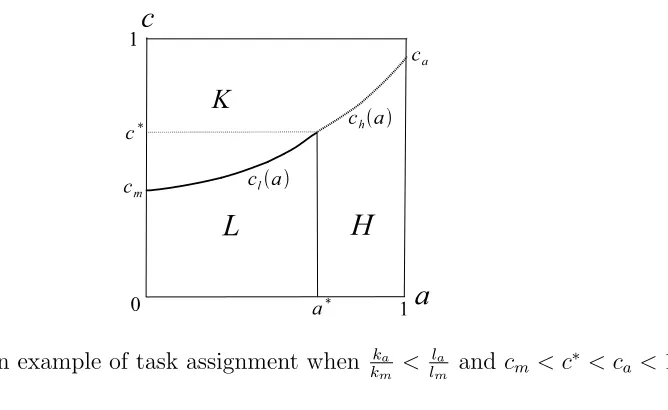
Figure 1: An example of task assignment when ka
km <
la
lm and cm < c
∗ < c
a<1
3
Analysis
This section derives task assignment and earnings explicitly, given machine abilities ka and
km. So far, no assumptions are imposed on comparative advantages of machines. Until
Section 5, it is assumed that ka
km <
la
lm(<
h
lm), that is, machines have comparative advantages in relatively manual tasks. Then, Al(a)
Ak(a) and
Ah(a)
Ak(a) increase with a. With this assumption, the task assignment conditions can be stated more explicitly.
3.1
Task assignment conditions
Remember that, fora < a∗, unskilled workers (machines) perform tasks (a, c) with Al(a)
cAk(a) > (<)wl
r, and for a > a
∗, skilled workers (machines) perform tasks (a, c) with Ah(a)
cAk(a) >(<)
wh
r ,
where a∗ is defined by Ah(a∗)
Al(a∗) =
wh
wl. Further, since
ka
km <
la
lm(<
h
lm), humans (machines) perform tasks with relatively high (low) a and low (high) c, and, for given c, machines perform tasks with a > a∗ only if they perform all tasks witha≤a∗. Based on this pattern
of assignment, critical variables and functions determining task assignment, cm, c∗, ca, cl(a),
and ch(a), are defined next. (Figure 1 may be useful in understanding the following.)
Unskilled workers vs. machines: From the above discussion, whenever nk(a, c) >0
for some (a, c),nk(0,1)>0, i.e. whenever machines are used, they perform the most manual
and easiest-to-codify task. Define cm as Al(0)
cmAk(0) =
lm
cmkm =
wl
r , i.e. cm is the value of c such
that hiring a machine and hiring an unskilled worker are equally profitable at task (0, cm).16
(Under the assumption ka
km <
la
lm, cm is the lowest c satisfying nk(a, c) > 0.) Then, other (a, c)s satisfying Al(a)
cAk(a) =
wl
r is given by Al(a)
cAk(a) =
lm
cmkm. Let cl(a) ≡
km
lm
Al(a)
Ak(a)cm. Given a, a machine and an unskilled worker are equally profitable atc=cl(a) and the former (latter) is
hired for c > (<)cl(a). If there exists c < 1 such that they are equally profitable at a=a∗,
i.e. cl(a∗) = klmm
Al(a∗)
Ak(a∗)cm < 1, machines perform some tasks with a > a
∗. If c
l(a∗) ≥ 1,
machines do not perform any tasks witha > a∗.Let c∗ ≡min{c
l(a∗),1}. 16
Skilled workers vs. machines: When c∗ < 1, the choice between a machine and a
skilled worker arises. Since Ah(a∗)
Al(a∗) =
wh
wl, (a, c)s satisfying
Ah(a)
cAk(a) =
wh
r is given by Ah(a)
cAk(a) =
lm
km
Ah(a∗)
Al(a∗)
1
cm and letch(a)≡
km
lm
Al(a∗)
Ah(a∗)
Ah(a)
Ak(a)cm. Givena, hiring either factor is equally profitable atc=ch(a). Ifc <1 exists such that either choice is equally profitable ata= 1, i.e. ch(1) =
h ka
km
lm
Al(a∗)
Ah(a∗)cm <1, machines perform some tasks with a = 1. Letca≡min{ch(1),1}. Figure 1 illustrates task assignment on the (a, c) space, assuming cm < c∗ < ca < 1.
Given a, machines perform tasks with higher c. From the assumption that machines have comparative advantages at relatively manual tasks, for given c, they perform tasks with lower a and the proportion of tasks performed by machines decreases with a, i.e. cl(a) and
ch(a) are upward sloping. These properties hold when cm < c∗ < ca<1 is not true too.
3.2
Key equations determining equilibrium
From their definitions, cl(a), ch(a), c∗,and ca are functions of cm and a∗:
cl(a) =
km
lm
Al(a)
Ak(a)
cm, ch(a) =
km
lm
Al(a∗)
Ah(a∗)
Ah(a)
Ak(a)
cm, (11)
c∗ ≡min{cl(a∗),1}, ca ≡min{ch(1),1}. (12)
From the equations defining a∗ and c
m, earnings too are functions of cm and a∗:
wl =
lm
km
r cm
, wh =
lm
km
Ah(a∗)
Al(a∗)
r cm
. (13)
Hence, the two key equations determining equilibrium, the first equality of (8) and (10), can be expressed as equations of cm and a∗ (refer to Figure 1 for the derivation):
Nh
Nl
∫ a∗ 0
∫ min{cl(a),1}
0
1
Al(a)
dcda=
∫ 1
a∗
∫ min{ch(a),1}
0
1
Ah(a)
dcda, (HL)
lm
km
r cm
∫ a∗ 0
∫ min{cl(a),1}
0
dcda Al(a)
+lm
km
Ah(a∗)
Al(a∗)
r cm
∫ 1
a∗
∫ min{ch(a),1}
0
dcda Ah(a)
+r
[∫ a∗
0 ∫ 1
min{cl(a),1}
dcda cAk(a)
+
∫ 1
a∗
∫ 1
min{ch(a),1}
dadc cAk(a)
]
= 1, (P)
Once a∗ and c
m are determined from (HL) and (P), c∗, ca, cl(a), ch(a) and thus task
assignment are determined. en, earnings are determined from (13), and the remaining variables are determined as stated in the definition of equilibrium.
The determination of equilibrium a∗and c
m can be illustrated using a figure depicting
graphs of (HL) and (P) on the (a∗, c
m) space. Since, as explained below, the shape of (HL)
differs depending on whetherc∗ andc
aequal 1 or not, using (11) and (12), the (a∗, cm) space
is divided into three regions based on values of c∗ and c
a, as illustrated in Figure 2.
In the figure, when cm ≥ klmm
Ak(a∗)
Al(a∗) ⇔
Al(a∗)
1×Ak(a∗) ≥
lm
cmkm =
wl
r, that is, when an unskilled
worker is weakly chosen over a machine at task (a, c) = (a∗,1), machines are not used in any
tasks witha > a∗ and thusc∗ =c
a = 1 holds. Whencm ≥ klmm
ka
h Ah(a∗)
Al(a∗) ⇔
h
1×ka ≥
lm
cmkm
Ah(a∗)
Al(a∗) =
wh
r andcm < lm
km
Ak(a∗)
Al(a∗), that is, when a skilled worker is weakly chosen over a machine at task (a, c) = (1,1) and a machine is strictly chosen over an unskilled worker at task (a, c) = (a∗,1),
machines are employed in some tasks with a > a∗ but not in tasks with a = 1 and c < 1,
thusc∗ < c
a= 1 holds. Finally, whencm < klmm
ka
h Ah(a∗)
Al(a∗), machines are employed in some tasks with a= 1 and c <1 and thusc∗ < c
Figure 2: Values of c∗ and c
a on the (a∗, cm) space when kkma <
la
lm
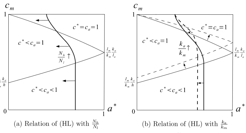
(a) Relation of (HL) with Nh
Nl (b) Relation of (HL) with
ka
km Figure 3: Shape of (HL) and its relations with Nh
Nl and
ka
km
3.3
Shape of
(
HL
)
and its relations with exogenous variables
The shape of (HL) and its relations with exogenous variables, NhNl and
ka
km, are illustrated in Figure 3, based on Lemmas 1−3 in Appendix A. Note that the shape and the relations do
not depend on the assumption ka
km <
la
lm, except that the casec
∗=c
a= 1 (the upper region in
the figure) does not arise when ka
km ≥
la
lm and the case c
∗ < c
a = 1 (the middle region) does
not arise when ka
km ≥
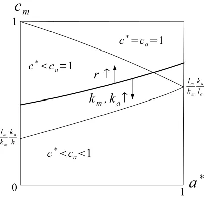
[image:12.612.94.520.347.578.2]Figure 4: Shape of (P) and its relations withkm, ka, and r
The left figure shows that (HL) is negatively sloped when ca= 1 and is vertical when
ca<1 on the (a∗, cm) space. The shape can be explained intuitively as follows. A decrease in
cmlowerscl(a) andch(a) from (11) and raises the proportion of tasks performed by machines
(see Figure 1). When ca= 1, i.e. machines do not perform any tasks with a= 1 and c <1,
the mechanization mainly affects unskilled workers engaged in relatively manual tasks and thus they shift to more analytical tasks, i.e. a∗ increases. By contrast, when c
a<1, both
types of workers are equally affected and thus a∗ remains unchanged.
The right figure illustrates the relations of (HL) with Nh
Nl and
ka
km. An increase in
Nh
Nl implies that a higher portion of tasks must be engaged by skilled workers and thus (HL) shifts to the left. Less straightforward is the effect of an increase in ka
km, which shifts the locus to the right (left) when cm is high (low), definitely so when c∗ = 1 (when ca <1).
An increase in ka
km weakens comparative advantages of humans in analytical tasks and thus lowers, particularly for high a, cl(a), ch(a), and the portion of tasks performed by humans
(see Figure 1). Whencm(thusc∗andca) is high, such mechanization mainly affects unskilled
workers and thus a∗ must increase, while the opposite is true when c
m is low.
3.4
Shape of
(
P
)
and its relations with exogenous variables
Figure 4 illustrates the shape of (P) and its relations with exogenous variables,km ka,andr,
based on Lemma 4 in Appendix A. Remember that, for (P) to hold, task assignment must be determined so that the unit production cost of the final good equals 1. Whencmincreases,a∗
must increase, that is, (P) is upward-sloping on the (a∗, c
m) plane, because, otherwise, both
wl=klmm
r
cm and wh=
Ah(a∗)
Al(a∗)wl fall and thus the unit production cost decreases. An increase in r raises the cost of hiring machines and thus a higher portion of tasks are assigned to humans, i.e. the locus shifts upward, while the opposite holds when abilities of machines,km
and ka, increase. The locus never intersects with cm = 0, because machines are completely
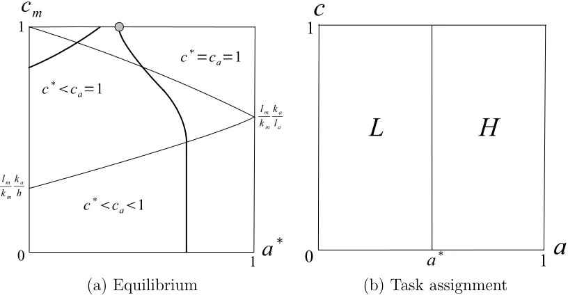
Figure 5: Determination of equilibrium a∗ and c
m
As Figure 5 illustrates, equilibrium (a∗, c
m) is determined at the intersection of the two
loci. Of course, the position of the intersection depends on exogenous variables such as km
andka. The next two sections examine how increases inkm,ka,and N
h
Nl affect the equilibrium, particularly, task assignment, earnings, earnings inequality, and aggregate output.
4
Mechanization with constant
kakm
Suppose that abilities of machines,km and ka, improve exogenously over time. This section
examines effects of such productivity growth and of an increase in Nh
Nl on task assignment, earnings levels and inequality, and output, when km andkasatisfying kkma <
la
lm grow propor-tionately. Since (HL) does not shift under constant ka
km (Figure 3 (a)), the analysis is much simpler than the general case analyzed in the next section.
The next proposition presents the dynamics of the critical variables and functions deter-mining task assignment of an economy undergoing the productivity growth.
Proposition 1Suppose that km and kasatisfying kkma <
la
lm grow over time with
ka
km constant. (i)When km is very low initially, cm =c∗ =ca = 1 is satisfied at first;17 at some point,
cm< c∗=ca= 1 holds and thereafter cm falls over time; then, cm< c∗< ca= 1 and c∗ too
falls; finally, cm< c∗< ca<1 and ca falls as well.
(ii)a∗ increases over time when c
m< ca= 1, while a∗ is time-invariant when ca < 1 (and
when cm= 1).
(iii)cl(a) and ch(a) (when c∗<1) decrease over time when cm<1.
The results of this proposition can be understood using figures similar to Figure 5. When the level of km is very low, there are no (a∗, cm) satisfying (P), or (P) is located at the left
17
(a) Equilibrium (b) Task assignment Figure 6: Equilibrium and task assignment when cm =c∗ =ca = 1
side of (HL) on the (a∗, c
m) plane (see Figure 6 (a)). Hence, the two loci do not intersect and
an equilibrium with cm<1 does not exist. Because the manual ability of machines is very
low, hiring machines is not profitable at all and thus all tasks are performed by humans. Figure 6 (a) illustrates an example of the determination of equilibrium cm and a∗ in this
case. Equilibrium a∗ is determined at the intersection of (HL) with c
m= 1. Figure 6 (b)
illustrates the corresponding task assignment on the (a, c) plane, which shows that unskilled (skilled) workers perform all tasks with a <(>)a∗.
When km becomes high enough that (P) is located at the right side of (HL) at cm= 1,
the two loci intersect and thus machines begin to be used, i.e. cm<1. Note that ka is not
important for the first step of mechanization, because mechanization starts from the most manual tasks in which analytical ability is of no use. Because of low machine productivities, they perform only highly manual and easy-to-codify tasks that were previously performed by unskilled workers, i.e. c∗=c
a= 1 holds. Indeed, large-scale mechanization originated in
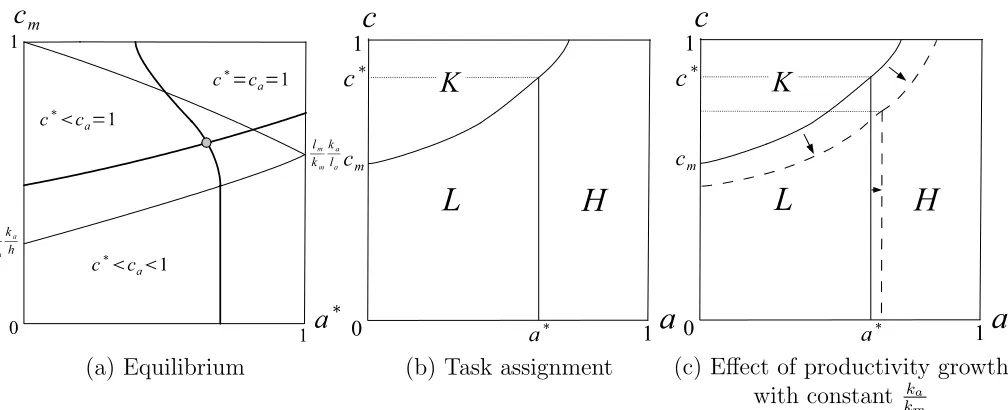
tasks associated with simple repetitive motions in textile during the Industrial Revolution. Figure 7 (a) and (b) respectively illustrate the determination of equilibrium cm and a∗ and
task assignment. Figure 7 (c) presents the effect of small increases in km and ka on the task
assignment. Since machines come to perform a greater portion of highly manual and easy-to-codify tasks, a∗ increases and c
l(a) decreases, that is, workers shift to more analytical
and, for unskilled workers, harder-to-routinize tasks. Consistent with the model, during early stages of industrialization, humans shifted from manual tasks at farms and cottages toward manual tasks at factories and analytical tasks at offices and factories (generally associated with clerical, management, and technical jobs), and manual workers shifted to tasks involving more complex motions machines were not good at.
As km and ka grow over time, mechanization spreads to relatively analytical tasks, and
(a) Equilibrium (b) Task assignment (c) Effect of productivity growth with constant ka
[image:16.612.57.566.114.317.2]km
Figure 7: Equilibrium, task assignment, and the effect of productivity growth with constant
ka
km whencm < c
∗ =c
a = 1
(a) Equilibrium (b) Task assignment (c) Effect of productivity growth with constant ka
km Figure 8: Equilibrium, task assignment, and the effect of productivity growth with constant
ka
km whencm < c
∗ < c
[image:16.612.60.564.439.644.2](a) Equilibrium (b) Task assignment (c) Effect of productivity growth with constant ka
[image:17.612.56.570.90.293.2]km Figure 9: Equilibrium, task assignment, and the effect of productivity growth with constant
ka
km whencm < c
∗ < c
a <1
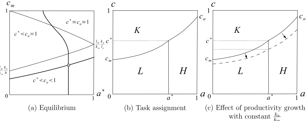
by skilled workers. In the real economy, the new phase of mechanization started during the Second Industrial Revolution − e.g. teleprinters replaced Morse code operators and tabulating machines substituted data-processing workers at large organizations− and has progressed on a large scale in the post World War II era, especially since the 1970s, because of the growth of IT technologies. Figure 8 (a) and (b) respectively illustrate the determination of equilibriumcm and a∗ and task assignment whencm< c∗< ca= 1. Machines perform some
tasks with a > a∗ but not the most analytical ones, i.e. c∗< c
a= 1. Productivity growth
lowers ch(a) as well as cl(a) (and raises a∗), thus skilled workers too shift to more
difficult-to-codify tasks (Figure 8 (c)). Congruent with the model, since the 1970s, humans have shifted from routine analytical tasks (such as simple information processing tasks typical in clerical jobs) as well as manual tasks toward non-routine analytical tasks mainly associated with professional and technical jobs and non-routine manual tasks in services.
Finally, the economy reaches the case cm < c∗ < ca<1, which is illustrated in Figure
9. Machines perform a portion of the most analytical tasks, i.e. ca<1. In fact, currently,
machines are engaged in some tasks involving analysis and decision-making, such as auto-mated trading in financial markets. Unlike the previous cases, productivity growth affects two type of workers equally and thusa∗ does not change, while c
h(a) and cl(a) decrease and
thus workers shift to more difficult-to-codify tasks. In sum, when the two abilities of machines with ka
km <
la
The dynamics of task assignment accord with the long-run trends of mechanization and of shifts in tasks performed by humans, except job polarization after the 1990s, which is detailed in the introduction and is summarized as: initially, mechanization proceeded in tasks intensive in manual labor, while mechanization of tasks intensive in analytical labor started during the Second Industrial Revolution and has progressed on a large scale in the post World War II era, especially since the 1970s, because of the growth of IT technologies; humans shifted from manual tasks to analytical tasks until about the 1960s, whereas, thereafter, they have shifted away from routine analytical tasks as well as routine manual tasks toward non-routine analytical tasks and non-routine manual tasks in services.
Effects of the productivity growth on earnings levels and inequality, and aggregate output are examined in the next proposition.
Proposition 2Suppose that km and ka satisfying kkma <
la
lm grow proportionately over time
when cm<1.
(i)Earnings of skilled workers increase over time. When c∗< c
a<1, earnings of unskilled
workers too increase.
(ii)Earnings inequality, wh
wl, rises over time when ca= 1 and is time-invariant when ca<1. (iii)The output of the final good, Y, increases over time.
The proposition shows that, while skilled workers always benefit from mechanization, the effect on earnings of unskilled workers is ambiguous when mechanization mainly affects them, i.e. when ca= 1, and the effect turns positive when ca<1. Mechanization worsens
earnings inequality, wh
wl, when ca= 1, while it has no effect when ca<1. The output of the final good always increases, even if la< h < lm and thus workers’ productivities, Ah(a) and
Al(a), fall as they shift to more analytical tasks.
So far, the proportion of skilled workers to unskilled workers, Nh
Nl, is held constant, which has increased over time in the actual economy. Thus, the next proposition examines effects of the growth of Nh
Nl under constant machine qualities.
Proposition 3Suppose that Nh
Nl grows over time when
ka
km<
la
lm and cm<1.
(i)cm, a∗,c∗ (whenc∗<1),andcl(a)decrease, while ca (whenca<1)andch(a) (whenc∗<1)
increase over time.
(ii)wl (wh) rises (falls) and earnings inequality, wwhl, shrinks over time.
(iii)Y increases over time under constant Nh+Nl.
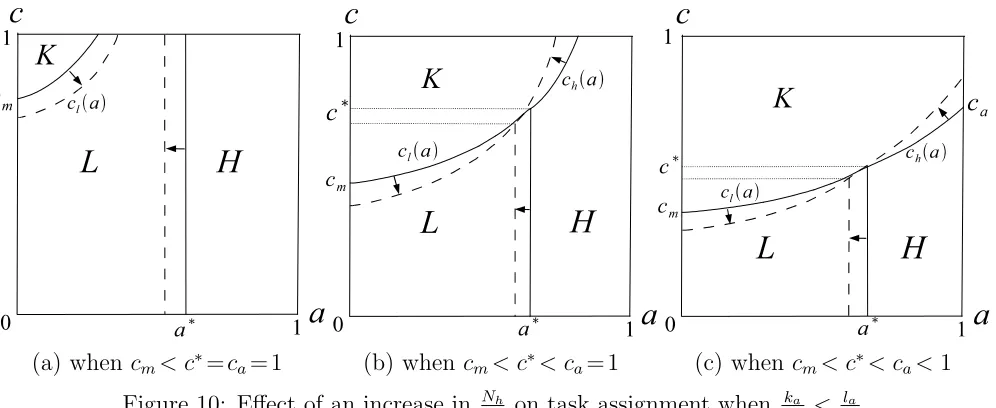
Figure 10 illustrates the effect of an increase in Nh
Nl on task assignment. Since skilled workers become abundant relative to unskilled workers, they take over a portion of tasks previously performed by unskilled workers, i.e. a∗ decreases. Further, earnings of unskilled
workers rise and those of skilled workers fall, thus some tasks previously performed by unskilled workers are mechanized, i.e. cl(a) decreases, while, when c∗<1, skilled workers
take over some tasks performed by machines before, i.e. ch(a) increases. That is, skilled
workers shift to more manual tasks, and unskilled workers shift to harder-to-routinize tasks. The output of the final good increases even when the total population is constant, mainly because skilled workers are more productive than unskilled workers at any tasks witha >0.
By combining the results on effects of an increase in Nh
(a) when cm< c∗=ca= 1 (b) when cm< c∗< ca= 1 (c) when cm< c∗< ca<1
Figure 10: Effect of an increase in Nh
Nl on task assignment when
ka
km <
la
lm
the 1970s (except the wartime 1940s) detailed in the introduction, which is: in early stages of industrialization when mechanization directly affected unskilled workers and the relative supply of skilled workers grew slowly, earnings of unskilled workers grew very moderately and earnings inequality rose; in later periods when skilled workers too were directly affected by mechanization and the relative supply of skilled workers grew faster, unskilled workers benefited more from mechanization, while, as before, the rising inequality was the norm in economies with lightly regulated labor markets (such as the U.S.), except in periods of a rapid increase in the level of education and in the 1940s, when the inequality fell.18
The model, however, fails to capture the trends after the 1980s, which is: earnings of unskilled workers stagnated and those of skilled workers rose until the mid 1990s in the U.S.;19 the inequality rose greatly after the 1980s (after the 1990s in many European
economies, OECD, 2008); and wage polarization has proceeded since the 1990s at least in the U.S. By contrast, the model predicts that earnings of unskilled workers increase and the inequality shrinks when highly analytical tasks are affected by mechanization, i.e. when
ca<1, and the relative supply of skilled workers rises.
5
Mechanization with time-varying
kakm
The previous section has examined the case in which km and ka grow proportionately. This
special case has been taken up first for analytical simplicity. However, the assumption of the proportionate growth is rather restrictive, because, according to the trend of mechanization
18
Combined effects of an increase in Nh
Nl and improvements of machine qualities on task assignment accord
with the trend of task shifts in the real economy when c∗= 1. Whenc∗<1, they are consistent with the
fact, unless the negative effect of an increase in Nh
Nl onch(a) is very strong (see Figure 10).
19
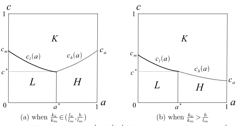
(a) when ka
km∈(
la
lm,
h
lm) (b) when
ka
km>
h lm(>
la
[image:20.612.104.522.89.304.2]lm) Figure 11: c∗ and c
a on the (a∗, cm) space when kkma ∈(
la
lm,
h
lm) and when
ka
km>
h lm(>
la
lm)
described in the introduction, the growth of km was apparently faster than that of ka in
most periods of time, while ka seems to have been growing faster thankm recently.20
This section examines the general case in which they may grow at different rates. This case is much more difficult to analyze because a change in ka
km shifts the graph of (HL) as well as that of (P) (see Figures 3 and 4). Under realistic productivity growth, the model does much better jobs in explaining the development after the 1980s than in the constant
ka
km case.
Unlike the previous case, shapes of graphs in Figures 1 and 2 may change qualitatively with productivity growth. Starting from the situation where ka
km<
la
lm(<
h
lm) holds, ifkakeeps growing faster thankm, i.e. the rapid growth of IT technologies is long-lasting, kkma ∈(
la
lm,
h lm), then ka
km >
h lm(>
la
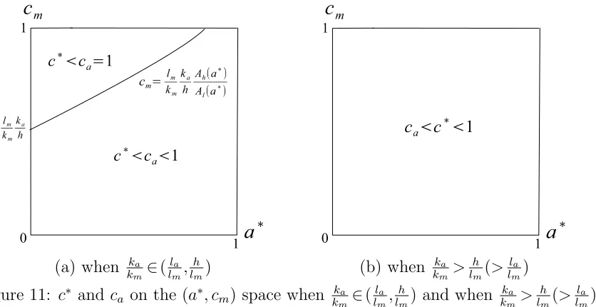
lm) come to be satisfied. That is, comparative advantages of machines to two type of workers change over time. As illustrated in Figure 11, when ka
km ∈(
la
lm,
h lm),
c∗ <1 holds, and when ka
km>
h lm(>
la
lm), ca < c
∗ <1 holds from c∗ = min{km
lm
Al(a∗)
Ak(a∗)cm,1
}
and
ca= min
{
h ka
km
lm
Al(a∗)
Ah(a∗)cm,1
}
.
Figure 12 illustrates cl(a) and ch(a) and task assignment on the (a, c) space when kkma ∈ (la
lm,
h
lm) (the figure is drawn assuming ca<1) and when
ka
km >
h
lm. Unlike the original case
ka
km<
la
lm,cl(a) is downward sloping and, when
ka
km>
h
lm,ch(c) too is downward sloping. Hence, when ka
km∈(
la
lm,
h
lm),for givenc, machines tend to perform tasks with intermediate a and the proportion of tasks performed by machines is highest at a =a∗. When ka
km>
h
lm, for given c, machines tend to perform relatively analytical tasks and the proportion of tasks performed by machines increases with a.
20
Note thatka seems to have been positive even before the Industrial Revolution. Various machines had
(a) when ka
km∈(
la
lm,
h
lm) (b) when
ka
km>
[image:21.612.107.506.85.294.2]h lm Figure 12: cl(a) and ch(a) when kkma ∈(
la
lm,
h
lm) (ca<1 is assumed) and when
ka
km>
h lm
5.1
Effects of changes in
k
m,
k
a,
and
NhNlNow, effects of changes in km and kaon task assignment, earnings levels and inequality, and
output are examined. Since results are different depending on the shape of (HL) (Figure 3), they are presented in three separate propositions.21,22The next proposition analyzes the
case c∗=c
a= 1, which arises only when kkma <
la
lm.
Proposition 4When cm≥klmm
Ak(a∗)
Al(a∗) ⇔c
∗=c
a= 1 (possible only when kkma <
la
lm), (i)cm decreases and a∗ increases with km and ka (limcm→1
da∗
dkm= limcm→1
da∗
dka= 0). (ii)cl(a) decreases with km and ka.
(iii)wh, w
h
wl, and Y increase with km and ka. wl increases with ka. The only difference from the constant ka
km case is that wl increases when ka rises with
km unchanged. As before, with improved machine qualities, cm and cl(a) decrease and a∗
increases, i.e. workers shift to more analytical and, for unskilled workers, harder-to-codify tasks, and earnings of skilled workers, earnings inequality wh
wl, and output rise. The next proposition examines the case c∗< c
a= 1, which is possible only when k
a
km<
h lm.
Proposition 5When cm∈
[
lm
km
ka
h Ah(a∗)
Al(a∗),
lm
km
Ak(a∗)
Al(a∗)
)
⇔c∗< c
a= 1 (possible only when kkma <
h lm), (i)cm decreases with km and ka. a∗ increases when kkma non-increases.
(ii)cl(a) and ch(a) decrease with km and ka.
(iii)wh and Y increase with km and ka, while wl increases with ka. wwhl increases when kkma
non-increases.
21
When ka
km > la
lm,cm= 1 is possible withc
∗ or ca <1. However, such situation −the most manual and
easy-to-codify task is not mechanized while some of other tasks are−is unrealistic and thus is not examined.
22
(a) when ka
km<
la
lm(<
h
lm) (b) when
ka
km∈(
la
lm,
h
lm) (c) when
ka
km>
[image:22.612.52.554.89.288.2]h lm Figure 13: Effect of productivity growth with increasing ka
km when cm < c
∗ < c
a <1
There are several differences from the constant ka
km case. First, effects of productivity growth with increasing ka
km on a
∗ and earnings inequality are ambiguous, and w
l increases
with ka. Second, although cl(a) (thus cm) and ch(a) decrease and thus workers shift to
harder-to-routinize tasks as in the original case, workers may not shift to more analytical tasks when a∗ decreases (possible only when ka
km increases) and when
ka
km ∈ (
la
lm,
h
lm) (see Figure 12 (a)). Remaining results are same as before, that is, when ka
km non-increases, a
∗
and earnings inequality increase; when ka
km ≤
la
lm too holds, workers shift to more analytical tasks; and earnings of skilled workers and output always increase.
Proposition 6 examines the case c∗, c
a<1 (c∗<(>)ca when kkma <(>)
h lm).
Proposition 6When cm < klmm
ka
h Ah(a∗)
Al(a∗) ⇔c
∗, c
a <1,
(i)cm and ca decrease with km and ka, and a∗ decreases with kkma. (ii)cl(a) and ch(a) decrease with km and ka.
(iii)wh and Y increase with km and ka, while wl increases when kkma non-decreases.
wh
wl
decreases with ka
km. Unlike the constant ka
km case,a
∗ and thus wh
wl decrease with
ka
km, and the effect onwl is am-biguous when ka
km decreases. As for task assignment, whilecl(a) (thuscm) andch(a) decrease as in the original case (thus workers shift to harder-to-routinize tasks), tasks performed by humans change in the skill dimension as well. In particular, when ka
km rises (falls), that is, when productivity growth is such that comparative advantages of machines to humans in analytical (manual) tasks rise, unskilled workers shift to more manual (analytical) tasks under ka
km>(<)
la
lm, and skilled workers too shift to such tasks under
ka
km>(<)
h lm.
23 Figure 13
23
When ka
km rises (falls) under ka km<(>)
la
lm, unskilled workers shift to more manual (analytical) tasks at
lowc. The same is true for skilled workers under ka
km<(>) h
lm. (See Figure 13.) Hence, at low c,workers
always shift to more manual (analytical) tasks when ka
(a) when ka
km∈(
la
lm,
h
lm) and ca= 1 (b) when
ka
km∈(
la
lm,
h
lm) andca<1 (c) when
ka
km>
[image:23.612.54.558.89.297.2]h lm Figure 14: Effect of an increase in Nh
Nl when
ka
km∈(
la
lm,
h
lm) and when
ka
km>
h lm
illustrates the effect of productivity growth with increasing ka
km on task assignment. Earnings of skilled workers and output rise as before.
Finally, Proposition 7 examines effects of an increase in Nh
Nl when
ka
km ≥
la
lm is allowed.
Proposition 7Suppose that Nh
Nl grows over time when cm<1.
(i)cm, a∗, and cl(a) decrease, while ca (when ca <1) and ch(a) (when c∗<1) increase over
time. c∗ (when c∗<1) falls (rises) when ka
km ≤
la
lm (
ka
km ≥
h lm). (ii)wl (wh) rises (falls) and wwhl shrinks over time.
(iii)Y increases over time under constant Nh+Nl.
Figure 14 illustrates the effect of an increase in Nh
Nl on task assignment when
ka
km∈(
la
lm,
h lm) and when ka
km >
h
lm. (Note thatc
∗=c
a= 1 does not arise in these cases andc∗< ca= 1 does not
arise when ka
km >
h
lm.) As in the original case of
ka
km <
la
lm, skilled workers take over some tasks previously performed by unskilled workers, i.e. a∗ decreases, and machines (skilled workers)
come to perform a portion of tasks performed by unskilled workers (machines) before, i.e.
cl(a) decreases (ch(a) increases). However, unlike before, cl(a) is downward-sloping on the
(a, c) plane, and, when ka
km >
h
lm, ch(a) too is downward-sloping. Thus, unskilled workers shift to harder-to-routinizeand more manual tasks, and skilled workers shift to more manual tasks only when ka
km∈(
la
lm,
h
lm) (see the figure). As in the original case, earnings of unskilled (skilled) workers rise (fall), earnings inequality shrinks, and output increases.
5.2
Contrasting the model with facts
Based on the propositions, it is examined whether the model with realistic productivity growth can explain the long-run trends of task shifts, earnings, and earnings inequality in the real economy. Two assumptions are imposed on comparative advantage of machines against humans and the relative growth of the machines’ two abilities. First, it would be plausible to suppose that ka
km <
la
ch(a) are downward-sloping on the (a, c) plane), since the proportion of tasks performed by
machines seems to have been and be higher in more manual tasks: consider the fact that the vast majority of non-routine analytical tasks generally associated with management, professional, and technical jobs and of non-routine ”middle a” tasks typical in occupations such as mechanics and nurses are yet to be mechanized. Second, the history of mechanization and task shifts described in the introduction suggests that km seems to have grown faster
than ka until sometime in the 1990s, after which the growth of ka appears to be faster
because of the growing application of IT technologies in many fields.24,25 (Note also that IT
technologies have contributed greatly to the growth of km too: industrial robots and CNC
[Computer Numerical Control] machines raised machines’ productivities to perform manual and relatively non-routine tasks considerably.) Thus, suppose that ka
km falls over time when
ca= 1, while, when ca<1, kkma falls initially, then rises.
Now, the dynamics of earnings and earnings inequality are examined. Since the result when c∗=c
a= 1 is almost the same as the constant kkma case, the model is consistent with the actual trends in the early stage of mechanization. The model accords with the trends in the intermediate stage as well (except a decline of the inequality in the wartime 1940s), because the result when c∗ =c
a <1 and kkma falls is same as before. Further, unlike the constant ka
km case, the model is congruent with stagnant earnings of U.S. unskilled workers in the 1980s and the early 1990s and the large inequality rise after the 1980s (after the 1990s in many European nations). This is because the effect of productivity growth with decreasing ka
km on their earnings is ambiguous and the effect on the inequality is positive when
c∗< c
a<1,and the growth of NNhl,which contributes to raising their earnings and lowering the
inequality, greatly slowed down during the period. When ka
km rises underc
∗< c
a<1, earnings
of unskilled workers too grow, which is consistent with the development in the late 1990s and the early 2000s.26 Although the model with two types of workers cannot explain wage
polarization after the 1990s observed at least in the U.S., the falling inequality predicted by the model captures a part of the development, the shrinking inequality between low-skill and middle-skill workers (most recently, mildly high-skill workers too).
As for the dynamics of task shifts, the result under c∗=c
a= 1 is same as the constant kkma case, and so is the result underc∗< c
a= 1 when kkma <
la
lm and
ka
km falls: cl(a) andch(a) decrease and a∗ increase over time, unless Nh
Nl grows rapidly. Hence, the dynamics accord with the long-run trend until recently, i.e. workers shift to more analytical and harder-to-routinize tasks over time. By contrast, when c∗ < c
a<1, while cl(a) and ch(a) decrease over time 24
It is true that several components of the composite analytical abilityka, such as numerical ability, seems
to have been growing faster than the composite manual abilitykmfor much longer periods. But remaining
components, such as analysis and decision-making abilities, seem to have grown slowly until recently.
25
The supposed turning point would be not be far off the mark considering that a decrease in the em-ployment share of production occupations, which are intensive in manual tasks, is greatest in the 1980s and slowed down considerably after the 1990s, while a decrease in the share of clerical occupations intensive in routine analytical tasks accelerated after the 1990s, according to Acemoglu and Autor (2011).
26
(unless Nh
Nl grows rapidly) as before, unlike the constant
ka
km case, a
∗ increases (decreases)
when ka
km falls (rises). Hence, workers shift to more analytical and harder-to-routinize tasks while ka
km falls, whereas after
ka
km starts to rise, they shift to harder-to-codify tasks overall and shift to more manual tasks at low c (footnote 23). This is consistent with the shift fromnon-routine analytical tasks as well as routine tasks to non-routine manual tasks after around the year 2000 in the U.S. (Beaudry, Green, and Sand, 2013; see footnote 10 in the introduction for details).
In sum, unlike the proportionate growth case, the model with realistic productivity growth is consistent with a large part of the development after the 1980s, including several aspects of job and wage polarization after the 1990s.
If the rapid progress of IT technologies continues and ka
km keeps rising, comparative ad-vantages of machines to two type of workers could change over time, i.e. first, from ka
km<
la
lm to ka
km∈(
la
lm,
h
lm), then to
ka
km>
h
lm. The model predicts what will happen to task assignment, earnings, and earnings inequality under such situations. As before, both types of workers shift to tasks that are more difficult to routinize (unless Nh
Nl rises greatly, which is very un-likely). By contrast, unlike before, unskilled workers shift to more manual tasks (even at high c), and, when ka
km>
h
lm, skilled workers too shift to such tasks (see Figures 13 and 14). That is, workers will shift to relatively manual and difficult-to-codify tasks: the recent shift to low-wage service occupations such as personal care and protective service may continue into the future. Earnings of unskilled workers as well as those of skilled workers will rise, and earnings inequality will shrink over time. The analysis based on the model with two types of workers may not capture the whole picture, considering the recent widening inequal-ity between mildly and extremely high-skill workers. However, episodes such as declining newspaper industry, burgeoning online education, and the increasing use of ”big data” in marketing and other management decisions suggest that machines will replace a large num-ber of tasks presently performed by highly skilled workers in the not-distant future and thus possible effects on a great majority of the population may be captured by the present model.
6
Conclusion
Since the Industrial Revolution, mechanization has strongly affected types of tasks humans perform, relative demands for workers of different skill levels, earnings levels and inequality, and aggregate output. This paper has developed a Ricardian model of task assignment and examined how improvements of qualities of machines and an increase in the relative supply of skilled workers affect these variables. The analysis has shown that tasks and workers strongly affected by the productivity growth and the effects on earnings and the inequality change over time. The model is consistent with long-run trends of these variables in the real economy, except a sharp decline of the inequality in the wartime 1940s and job and wage polarization after the 1990s, which is beyond the scope of the model with two types of workers, although the model does capture an important part of the latter development. The model has also been employed to examine possible future trends of these variables when the rapid growth of IT technologies continues.
more than two type of workers, who differ in levels of analytical ability or ability to perform non-routine tasks, could be developed. Second, empirical works find that international trade and offshoring have important effects on earnings inequality,27 thus it may be interesting to
examine effects of these factors and productivity growth jointly.
References
[1] Acemoglu, D. and D. Autor (2011), ”Skills, Tasks and Technologies: Implications for Employment and Earnings,” in O. Ashenfelter and D. Card, eds., Handbook of Labor Economics Volume IV, Part B, Amsterdam: Elsevier, Chapter 12, 1043−1171.
[2] Acemoglu, D. and F. Zilibotti (2001), ”Productivity Differences,” Quarterly Journal of Economics 116, 563−606.
[3] Autor, D., F. Levy and R. Murnane (2002), ”Upstairs, Downstairs: Computers and Skills on Two Floors of a Large Bank,” Industrial and Labor Relations Review 55 (3), 432−447.
[4] Autor, D., F. Levy and R. Murnane (2003), ”The Skill Content of Recent Technological Change: An Empirical Exploration,” Quarterly Journal of Economics 116 (4).
[5] Autor, D., L. Katz, and M. Kearney (2006), “The Polarization of the U.S. Labor Mar-ket,”American Economic Review Papers and Proceedings 96 (2), 189−194.
[6] Bartel, A., C. Ichniowski, and K. Shaw (2007), ”How Does Information Technology Affect Productivity? Plant-Level Comparisons of Product Innovation, Process Improve-ment, and Worker Skills,” Quarterly Journal of Economics 122(4), 1721−1758.
[7] Beaudry, P., D. Green, and B. Sand (2013), “The Great Reversal in the Demand for Skill and Cognitive Tasks,” NBER Working Paper No. 18901.
[8] Costinot, A. and J. Vogel (2010), “Matching and Inequality in the World Economy,”
Journal of Political Economy 118 (4), 747−786.
[9] Feinstein, C. H. (1998), ”Pessimism Perpetuated: Real Wages and the Standard of Living in Britain during and after the Industrial Revolution,” Journal of Economic History 58(3), 625−658.
[10] Firpo, S., N. Fortin, and T. Lemieux (2011), “Occupational Tasks and Changes in the Wage Structure,” mimeo, University of British Columbia.
[11] Givon, D. (2006), ”Factor Replacement versus Factor Substitution, Mechanization and Asymptotic Harrod Neutrality,” mimeo, Hebrew University.
[12] Garicano, L. and E. Rossi-Hansberg (2006), ”Organization and Inequality in a Knowl-edge Economy,”Quarterly Journal of Economics 121 (4), 1383−1435.
[13] Goldin, C. and L. F. Katz (1998), ”The Origins of Technology-Skill Complementarity,”
Quarterly Journal of Economics, 113 (3), 693−732.
27