Munich Personal RePEc Archive
Dynamic State-Space Models
Karapanagiotidis, Paul
University of Toronto, Department of Economics
3 June 2014
Dynamic State-Space Models
∗
Paul Karapanagiotidis
†Draft 6
June 3, 2014
Abstract
A review of the general state-space modeling framework. The discussion focuses heavily on the three prediction problems of forecasting, filtering, and smoothing within the state-space context. Numerous examples are provided detailing special cases of the state-state-space model and its use in solving a number of modeling issues. Independent sections are also de-voted to both the topics of Factor models and Harvey’s Unobserved Components framework.
Keywords: state-space models, signal extraction, unobserved components. JEL: C10, C32, C51, C53, C58
1
Introduction
The dynamic state-space model was developed in the control systems literature, where
physi-cal systems are described mathematiphysi-cally as sets of inputs, outputs, and state variables, related
by difference equations. The following, Section 2, describes the various versions of the linear
state-space framework, discusses the relevant assumptions imposed, and provides examples
en-countered in economics and finance. Subsequently, Section 3 provides the analogous description
of the more general nonlinear state-space framework. Section 4 then discusses some of the
com-mon terminologies related to the state-space framework within the different contexts they are
encountered. Section 5 follows by discussing the general problems of state-space prediction,
including forecasting, filtering, and smoothing. Moreover, it provides a number of simple
ap-plications to chosen models from Section 2. Sections 6 and 7 then go into more detail: Section
6 briefly discusses the problem of prediction in the frequency domain and Section 7 outlines in
detail the solutions to the forecasting, smoothing, and filtering problems, within the time domain.
In particular, we interpret the solutions in terms of an orthogonal basis, and provide the MA
and AR representations of the space model. Section 8 then details estimation of the
state-space model parameters in the time domain. Finally, Section 9 discusses the equivalent Factor
model representation, including the relationship between this representation, the VARMA, and
the VECM models. It also discusses in more detail the Unobserved Components framework
popularized by Harvey (1984,89).
2
Linear dynamic state-space model
2.1
The models
2.1.1 Weak linear state-space model
The weak form of the lineardynamic state-space modelis as follows:
xt=Ftxt−1+ǫt, (1a)
yt=Htxt+ηt, (1b)
with the moment restrictions:
E[ǫt] =0, Cov(ǫt,ǫt−s) =Σǫt✶s=0, (2a)
E[ηt] =0, Cov(ηt,ηt−s) = Σηt✶s=0,
E[ǫt−jη′t−s] =0, ∀j, s∈Z,
and Cov(x0,ǫt) =Cov(x0,ηt) =0, ∀t >0,
where:
◦ xtis ap×1vector of state process values at timet.1
◦ ǫtandηtare assumed uncorrelated with each other across all time lags, and their covariance
matrices,ΣǫtandΣηt, depend ont.
◦ Ft is called the “system matrix” and Ht the “observation matrix.” These matrices are
assumed to benon-stochasticwhereFt isp×p, and if we allow for more state processes
than observed ones,Htisn×pwheren≥p.
◦ Equation (1a) is called the “state transition” equation and (1b) is called the “observation”
or “measurement” equation.
◦ The state initial condition, x0, is assumed stochastic with second order moments denoted
E[x0] = µandV ar(x0) = Σx0. Finally, there exists zero correlation between the initial
state condition and the observation and state error terms, for all datest >0.
2.1.2 The Gaussian linear state-space model
In the weak version of the linear dynamic state-space model, the assumptions concern only the
first and second-order moments of the noise processes and initial state, or equivalently the first
and second-order moments of the joint process[(x′t,y′t)′]. We can also introduce a more
restric-tive version of the model by assuming, independent, and identically distributed, Gaussian white
noises (IIN) for the errors of the state and measurement equations. The Gaussian linear state
1
space model is therefore defined as:
xt=Ftxt−1+ǫt, (1a)
yt=Htxt+ηt, (1b)
where
ǫt
ηt
t≥1
∼IIN
0
0
,
Σǫt 0
0 Σηt
, x0 ∼N(0,Σx0), (3a)
and x0 and the joint process (ǫt,ηt) are independent.
The Gaussian version of the state-space model is often used as a convenient intermediary tool.
Indeed, under the assumption of Gaussian noise and initial state, we know that the joint process
[(x′
t,y′t)′] is Gaussian. This implies that all marginal and conditional distributions concerning
the components of these processes are also Gaussian. If the distributions are easily derived, we
get as a by-product the expression of the associated linear regressions and residual variances.
Since these linear regressions and residual variances are functions of the first and second-order
moments only, their expressions are valid even if the noises are not Gaussian–that is, for the weak
linear state space model.
2.2
Examples
We will now discuss various examples of the state-space model. The first examples from
2.2.1-2.2.3 are descriptive models used for predicting the future; the second set of examples,
2.2.4-2.2.9 introduces some structure on the dynamics to capture measurement error, missing data,
or aggregation. Finally, the last examples, 2.2.10-2.2.12, come from economic and financial
2.2.1 The Vector Autoregressive model of order 1, VAR(1)
The (weak) Vector AutoRegressive model of order 1,V AR(1), is defined as:
xt =F xt−1+ǫt, with ǫt∼W W N(0,Σǫ), (4a)
yt =xt, (4b)
with the condition of no correlation between initial state, x0, and the error terms, ǫt, satisfied.
Furthermore, W W N denotes “weak white noise” or a process with finite, constant, first and second-order moments which exhibits no serial correlation.
In this case the observation process coincides with the state process. This implies that:
yt =F yt−1+ǫt, with ǫt ∼W W N(0,Σǫ), (5)
which is the standard definition of the (weak)V AR(1)process.
2.2.2 The univariate Autoregressive model of orderp, AR(p)
The (weak) univariate AutoRegressive model of orderp,AR(p), is defined as:
xt+b1xt−1 +· · ·+bpxt−p =ǫt, with ǫt∼W W N(0, σǫ2), (6)
The model can be written in state-space form as:
xt=F xt−1+ǫt, (7a)
yt=Hxt. (7b)
The state vector includes the current and firstp−1lagged values ofxt:
xt =
xt xt−1 . . . xt−p+1
′
p×1
with system matrices are given as: F =
−b1 −b2 . . . −bp−1 −bp
1 0 . . . 0 0 0 1 . . . 0 0
..
. ... . .. ... ...
0 0 . . . 1 0
p×p
, (9a)
H =
1 0 . . . 0
1×p
, (9b)
and ǫt =
ǫt 0 . . . 0
′
p×1
. (9c)
Since theAR(p) process is completely observed, ηt = 0and Σηt = 0 for allt. Moreover,
Σǫt is a singular matrix with zeroes in each element except the top diagonal element, which is
equal toσ2
ǫ for allt.
2.2.3 The univariate Autoregressive-Moving Average model of order(p, q), ARMA(p,q)
The (weak) univariate AutoRegressive-Moving Average model of order(p, q), ARM A(p, q), is defined as:
xt+b1xt−1+· · ·+bpxt−p =ǫt+a1ǫt−1+· · ·+aqǫt−q, where ǫt ∼W W N(0, σǫ2), (10)
There are a number of possible state-space representations of an ARMA process. In the language
of Akaike (1975), a “minimal” representation is a representation whose state vector elements
represent the minimum collection of variables which contain all the information needed to
pro-duce forecasts given some forecast origin t. For ease of exposition in what follows we provide a non-minimal state-space representation, although the interested reader can consult Gourieroux
Let the dimension of the statextbem=p+q. We have:
xt=F xt−1+Gǫt, (11a)
yt=Hxt, (11b)
The state vector is given as:
xt=
xt xt−1 . . . xt−(p−2) xt−(p−1) ǫt ǫt−1 . . . ǫt−(q−2) ǫt−(q−1)
′
. (12a)
The system matrices are given as:
F =
−b1 . . . −bp−1 −bp a1 . . . aq−1 aq
1 0 . . . 0 0 0 . . . 0 0 1 . . . 0 0 0 . . . 0
..
. ... . .. ... ... ... . . ... 0 0 . . . 1 0 0 . . . 0 0 0 . . . 0 0 0 . . . 0 0 . . . 0 0 1 0 . . . 0 0
..
. . . ... ... 0 1 . . . 0 0 ..
. . . ... ... ... ... . .. ... ... 0 . . . 0 0 0 0 . . . 1 0
m×m
, (13a)
G=
1 0 . . . 0 1 0 . . . 0
′
m×1
, (13b)
H =
1 0 . . . 0
1×m
, (13c)
and ǫt ≡ǫt∼W W N(0, σ2ǫ). (13d)
2.2.4 Partially observed VARMA
In the discrete-time multivariate case, suppose that some linear, unobserved, state process xtis
composed of filtered weak white noise ǫt. However, what we actually observe isyt, which has
been corrupted by additive weak white noiseηt. This model can be written as:
xt =
∞ X
u=0
auǫt−u =A(L)ǫt, (14a)
and yt =xt+ηt, for t = 1, . . . , T, (14b)
where:
◦ xtis an unobservedP ×1vector of state variables.
◦ the unobserved state xt (the “signal” in the engineering context) is corrupted with weak,
white, additive noise,ηt, with covariance matrixΣη.
◦ ǫtis anM×1vector of weak white noise input processes with covarianceΣǫ. 2
◦ ytis aP ×1vector of the observed “noisy” output process.
◦ ΣηandΣǫ represent the covariance of the measurement noise and the state process noise,
respectively, and are assumed time-invariant.
Note thatA(L)is a P ×M matrix infinite series whereL denotes the lag operator; that is,
A(L) = a0L0 +a1L1 +a2L2 +. . .. , where the individualP ×M matrices, au, collectively
represent the impulse response functionf wheref :Z→RP×M.
Given (14a), the infinite lag distribution makes working with this model in the time domain
troublesome. However, the apparent multi-stage dependence can be reduced to first-order
au-toregressive dependence by means of a matrix representation if we assume that A(L) can be well-approximated by a ratio of finite lag matrix polynomials – the so called “transfer function”
models of Box & Jenkins (1970). That is, suppose that we model instead:
C(L) =B(L)−1A(L)
= I +b1+b2L2+· · ·+bnLn)
−1
a0+a1+a2L2+· · ·+an−1Ln−1)
(15)
where the inverse of the matrix lag polynomialB(L)is assumed to exist.
The model in (14), with the ratio of finite order matrix lag polynomialsC(L)now replacing the infinite seriesA(L), becomes:
xt+b1xt−1, . . . ,+bnxt−n=a0ǫt+, . . . ,an−1ǫt−(n−1), ∀t= 1, . . . , T, (16a)
and yt=xt+ηt, (16b)
(16) can now be reduced to first-order dependence by means of a redefinition of the state
vector as:
x∗t =Txˆt−1, (17a)
where T =
−bn 0 0 . . . 0
−bn−1 −bn 0 . . . 0
−bn−2 −bn−1 −bn . . . 0
..
. . .. 0
−b1 −b2 −b3 . . . −bn
P n×P n
, (17b)
and xˆ′t−1 =
x′t−1 x′t−2 . . . x′t−n
1×P n
, (17c)
so that the new first-order autoregressive state-space model takes the form:
x∗t =F x∗t−1+Gǫˆt, (18a)
where we have that: F =
0 0 . . . 0 −bn I 0 . . . 0 −bn−1
..
. ... ... ...
0 0 . . . I −b1
P n×P n
, (19a) G=
0 0 0 0
..
. ... ... ...
a0 a1 . . . an−1
P n×M n
, (19b)
H =
0 0 . . . I
P×P n
, (19c)
and ˆǫ′t =
ǫ′t ǫ′t−1 . . . ǫ′t−(n−1)
1×M n
(19d)
where again F is the “system matrix,” G the “input matrix,” and H the “observation
ma-trix.” Bear in mind that (18) and (19) represent only one possible state-space representation
– in fact while the transfer function C(e−iω) in h
xx(ω) (see Section 2.2.4, (20a)) implies an
infinite number of possible state-space representations, any particular state-space
representa-tion has only one equivalent transfer funcrepresenta-tion. Addirepresenta-tionally, we can immediately see from
(18b) that the observed process yt is a linear function of the unobserved “factors” since yt =
−b1xt−1−b2xt−2− · · · −bnxt−n+ut+ηt, whereutis equal to the right-hand side of (16a).
See Akaike (1974) for a general treatment of finite order linear systems.
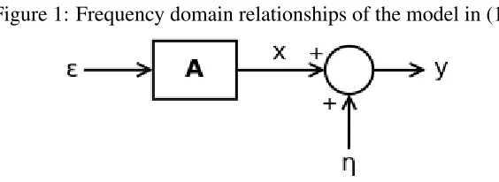
i) Spectral properties of the partially observed VARMA process
Note that from (14a), A(L) = P∞u=0auLu, so A(L)ǫt = P∞u=0auǫt−u More generally, A(z) = P∞u=0auzu where z ∈ C is known as the z-transform. Therefore, while A(L) is
a polynomial function of an operator L, the z-transform, A(z), is a polynomial function of a complex variable. However, since both polynomials admit the same coefficients, we can solve
transform of the impulse response function.3 (Note that in continuous time this z-transform
analogy is unnecessary since there is no need for defining the model in terms of lag operators,L). Therefore, the convolution observed in the time domain in (14a) is equivalent to a multiplication
within the frequency domain, so that the Fourier transform of the impulse response, A(e−iω),
disentangles the complicated interdepencies into a simple multiplicative relation between inputs
and outputs given any frequency ω. Therefore, working with (14) in the frequency domain is often a useful approach. For clarity the frequency domain relationships are given diagramatically
[image:12.612.160.442.256.359.2]in Figure 1.
Figure 1: Frequency domain relationships of the model in (14)
Sinceǫtandηtare jointly stationary and uncorrelated we have that:
hyx(ω) =A(e−iω)hǫǫ(ω)A(e+iω)′ = 1 2πA(e
−iω)ΣǫA(e+iω)′ =hxx(ω), (20a)
and hyǫ(ω) =A(e−iω)hǫǫ(ω) =
1 2πA(e
−iω)Σ
ǫ (20b)
represent the cross-spectral density matrices betweenytandxt,ytandǫtrespectively. Therefore,
from (20a) it is clear thatxtrepresents “filtered” weak white noise, where the flat spectrum ofǫt
(i.e. its variance) is given shape byA(e±iω).
Furthermore, the spectral-density matrix ofytis (from (16)):
hyy(ω) =hxx(ω) +hηη(ω) = 1 2π A(e
−iω)ΣǫA(e+iω)′+Σ
η
. (21)
3The system in (14) is constrained to be “physically realizable” by assuming the impulse response matrices are
aj = 0, ∀j < 0. This form of impulse response exists, is unique, and is quadratically summable, with no zeros
inside the unit circle as long as the integral from−πtoπof the log ofǫt’s spectral density is finite – see Doob
Note that for the discrete time process all spectral densities are continuous in the frequencyω
and periodic with period2π.
Finally, a natural non-parametric estimator of the transfer function matrix is given by:
ˆ
A(e−iω) = ˆh
yǫ(ω) ˆh−ǫǫ1(ω) = 2πhˆyǫ(ω)Σdǫ−1 (22)
where the spectral densities in (22) can be estimated within the frequency domain. See Priestley
(1981, Section 9.5) for more details.
Now, suppose we wish to establish the optimal manner of extracting the signal xt given
only the noisy observationsyt. That is, we wish to establish the optimal frequency response, or
transfer function C(ω), in Figure 2. It was Wiener that original solved this frequency domain problem where he established the optimal frequency response as the ratio:4
C(ω) = hxy(ω)
hyy(ω) =
hxx(ω)
hxx(ω) +hηη(ω). (23)
Therefore, the Wiener filter attenuates those frequencies in which the signal to noise ratio is low
and passes through those where it is high.
Figure 2: Wiener filter - the optimal transfer functionC(ω)
4Noting of course that sinceE[x
tx′t−s]is symmetric in the time domain for alls, we have thathxx(ω)is real,
2.2.5 The VAR(1) with measurement error
A special case of the partially observed VARMA model in Section 2.2.4 arises as the (weak)
VAR(1) with measurement error is defined as:
xt=F xt−1+ǫt, (24a)
yt=xt+ηt, (24b)
ǫt
ηt
t≥1
∼W W N
0
0
,
Σǫ 0
0 Ση
, (24c)
with the condition of no correlation between initial state,x0, and the error terms process, (ǫt,ηt),
satisfied.
Therefore, the state-space process is a VAR(1) process, but measured with a multivariate error
given byηt. The process (yt) is such that:
yt−F yt−1 =xt+ηt−F xt−1+ηt−1
=ǫt+ηt−F ηt−1 ≡vt (25a)
The process (vt) has serial covariances equal to zero for lags larger or equal to 2. Therefore,vt
admits a Vector Moving Average, VMA(1), representation of order 1. Letvt =ut−Θut−1.5 We
can therefore deduce that the process yt has a Vector Autoregressive-Moving Average of order
(1,1), or VARMA(1,1), representation:
yt−F yt−1 =ut−Θut−1, with ut∼W W N(0,Σu), (26)
ΘandΣuare functions of the intial parameters of the state-space representation: F,Σǫ,and
5And so we have that there exists no correlation between initial state,x
Ση. They are related by the matrix equations system:
−FΣη =ΘΣu (27a)
Ση+FΣηF′+Σǫ =Σu+ΘΣuΘ′ (27b)
which can be solved numerically for values ofΘandΣu.
2.2.6 Static state-space model
The (weak) static state-space model is defined as:
xt=ǫt, (28a)
yt=Hxt+ηt, (28b)
ǫt
ηt
t≥1
∼W W N
0 0 ,
Σǫ 0
0 Ση
, (28c)
with the condition of no correlation between initial state,x0, and the error terms, (ǫt,ηt),
satis-fied.
Therefore, from (28) the distribution of the state-space process is such that:
xt
yt
t≥1
=W W N
0 0 ,
Σǫ ΣǫH
′
HΣǫ HΣǫH′ +Ση
. (29)
In general, the state-space form is equivalent to the factor modelrepresentation, where we
assume that some pfactors, xt, influence the n observed processes yt, wheren > p. Indeed, the goal of the factor model representation is to model the observed processes in terms of a
smaller number of factor processes. Therefore, the particular form of the state-space model in
instead be formulated in a dynamic manner as in (1a).
We can distinguish two cases in practice:
◦ Case 1: the factorxtis unobserved.
In this case, the unrestricted theoretical model above is unidentifiable. This is because the
number of parameters exceeds the number of population moment conditions when xt is
unobserved. Indeed, from (29), we have:
V ar(yt)n×n =Hn×pΣǫp×pH′p×n+Σηn×n, (30)
and so then(n+ 1)/2population second moment conditions are outnumbered by thenp+
p(p+ 1)/2 +n(n+ 1)/2parameters.
Therefore, moment contraints on the parameters of the factor model are usually introduced
to ensure identification. For example, we can assume without loss of generality that the
factor covariance matrix,Σǫ, is an identity matrix. Indeed, xt is unobserved and defined
up to an invertible linear transform. That is, for any invertible matrix Lequation (28b)
with x∗t = Lxt and H∗ = HL−1 is observationally equivalent. Therefore, for any Σǫ
we can always introduce the transformationx∗t =D−1/2P′xt, where the matrixP has an
orthonormal basis of eigenvectors ofΣǫ as its columns andD is a diagonal matrix of the
respective eigenvalues, so as to makeV ar(x∗
t) =I. Moreover, it is often assumed in the
literature that the observation error covariance matrix,Ση, is diagonal (or even scalar) so
thatΣη =ση2I. This additional constraint is considered a “real” constraint since it reduces
the model’s flexibility in favour of identification.
◦ Case 2: the factorxtis observed.
In this, case the unrestricted theoretical model becomes identifiable. Given the moment
conditionV ar(xt),Σǫis identified. We can then formulate the theoretical linear regression
The static factor model is popular in Finance, where the observed variableytrepresents the
returns of a set of assets. Under a (weak) efficients market hypothesis the returns are WWN.
The observation equation (28b) thus decomposes the returns into a market component,Hxt, and
a firm specific component, ηt. Assuming an uncorrelated market component, the unobserved
factors,xt, represent the returns on the market andηtrepresent the firm specific returns, whose
variability (or “indiosyncratic” risk) can be reduced through its addition to a well diversied
port-folio. Of course, the assumption of uncorrelated market component can be generalized within
the dynamic model. For more on the factor model representation, see Section 9.
2.2.7 The state-space model for “data aggregation”
Suppose that we assume the state vectorxtrepresents some individual level components which
we desire to aggregate in some way. In a model for aggregation you have to distinguish
be-tween both the behavioural equation which generally includes an error term, and the accounting
relationship with no error term.
Therefore, letytrepresent the observed aggregate variable, and letxtrepresent some possibly
unobserved individual level variables. The state-space formulation defines both the behavioural
equation forxtand the accounting equation forytas:
xt =F xt−1+ǫt, where ǫt∼W W N(0,Σǫ), (31a)
yt =α′xt, (31b)
whereα=
α1 α2 . . . αp
′
is apvector of size adjustment parameters (which may possibly sum to 1) and so we can model the observed values yt as the weighted aggregate of individual
factors, the elements ofxt.
Note that in an accounting relationship you can only add variables with the same unit.
There-fore, we have first to transform the elements ofxtinto a common unit, which is usually done by
The aggregation model can also be employed in the Finance context. In this case, as opposed
to Section 2.2.6, the observation equation represents an accounting relationship between asset
returns and the aggregate portfolio return, not a behavioural relationship. The returns may be
weighted according to their contribution to the overall portfolio, where again the returns are
written in the same domination, e.g. dollars.
2.2.8 The VAR(1) with “series selection” or “missing series”
The Vector AutoRegressive process of order 1, or VAR(1), with “series selection” or “missing
series” is defined as:
xt=F xt−1+ǫt, where ǫt∼W W N(0,Σǫ), (32a)
and yt=xi,t, (32b)
wherexi,t denotes the i’th element ofxt. Therefore the model can be interpreted in two ways,
depending on whether or notxtis observed:
◦ Case 1: xtis observed.
The model is then interpreted as a method of selecting only that series from the state vector
xtthat is of interest. Notice that (31b) above is a special case of series selection, whenxt
is observed.
◦ Case 2: xtis not observed.
The model is interpreted as the case of “missing series.” That is, some of the elements of
the series(xt)are missing.
2.2.9 The VAR(1) with “missing data”
The model in Section 2.2.8, with unobservedxt, can of course be generalized to the cases where
well. We call this the vector autoregressive process of order 1, or VAR(1), for “missing data”.
The state equation is the same for all cases below:
xt =F xt−1+ǫt, where ǫt∼W W N(0,Σǫ). (32a)
◦ Case 1: thei’th series is missing and some elements of thej’th series are missing:
yt=
x1,t . . . xi−1,t xi+1,t . . . xj,t . . . xp,t
′
if t6=m
x1,t . . . xi−1,t xi+1,t . . . xj−1,t xj+1,t . . . xp,t
′
if t=m
. (33)
◦ Case 2: thei’th and j’th series both have missing data but the missing points occur at the
same time:
yt=
xt if t6=m
x1,t . . . xi−1,t xi+1,t . . . xj−1,t xj+1,t . . . xp,t
′
if t=m
. (34)
◦ Case 3: thei’th andj’th series both have missing data with no inherent pattern.
Where in each case, m ∈ 0, . . . , T, denotes a time period upon which some elements of the vectorxtare missing.
2.2.10 The Unobserved Components model
Consider the special case of the state-space model for aggregation in Section 2.2.7, where the
elements ofαare all equal to one, and we assume that thepelements ofxtare independent of each other with specified marginal distributions or we at least specify their first two moments:
xt=F xt−1+ǫt, (35a)
yt=
1 . . . 1
the observed seriesytis therefore the sum of variouscomponents, generally unobserved.
2.2.10.1 The General Stochastic Trend
P.C. Young (2011, p.67) defines thegeneralized random walkor generalstochastic trendas:
xt =
x1,t
∆x1,t
, (36a)
xt =F xt−1+Gǫt, where F =
α β
0 γ
, and
δ 0
0 ǫ
. (36b)
Also ǫt∼W W N(0,Σǫ) where Σǫ is diagonal. (36c)
That is, we have defined the state process in such a manner as to allow us to modify the
behaviour of the typical random walk in different ways. For example, if β = γ = ǫ = 0and
α =δ = 1the model represents the standard random walk. However, ifα=β =γ =ǫ= 1and
δ = 0 we have theintegrated random walk which is smoother than the standard random walk.
Moreover, if 0 < α < 1 and β = γ = ǫ = 1 and δ = 0 we have the case of the smoothed random walk. Also the case of β = γ = ǫ = 0 and0 < α < 1andδ = 1is equivalent to the AR(1) model. Finally, both the Local Linear Trend (see Section 2.2.10.2) and Damped Trend
from Harvey (1984,89) are both given by α = β = γ = ǫ = δ = 1(except in the latter case 0< γ <1).
2.2.10.2 Harvey’s Unobserved Components models: the “basic structural model”
Harvey (1984,89) attempts to decompose the series (yt) into a number of unobserved, orthogonal,
informed by the spectral properties of the observed series. For example, consider the model:
yt=Tt+St+Ct+It (37)
whereyt is the observed series,Tt is some trend component, Stis a seasonal component, Ct is
some other cyclical component, andItrepresents the irregular pattern.
Typically the trend componentTtis associated with the slowly changing, low frequency
com-ponent ofyt (i.e. a spectral frequency close to zero, or equivalently a period close to∞). It can
be modeled by the stochastic counterpart of the linear time trendµt =µ0 +βt, called theLocal Linear Trendmodel:
Tt ≡µt=µt−1+βt−1+vt, where vt∼W W N(0, σ2v), (38a)
and βt=βt−1 +zt, where zt∼W W N(0, σ2z). (38b)
Of course, the Local Linear Trend formulation is a special case of the general stochastic trend in
Section 2.2.10.1.
Furthermore, the seasonal component St can be modeled as dummy intercepts which are
constrained to sum to zero (with some small stochastic residual difference, ω). For example, suppose s is the number of “seasons” (say 12 for monthly data) and zj,t for j = 1,2, . . . , sis
some set of dummy variables that take on the values:
zj,t =
1, if t=j, j+s, j+ 2s, . . .
0, if t6=j, j+s, j+ 2s, . . .
−1, if t=s,2s,3s, . . .
then, ifγj is the dummy intercept for timej, we have that att=xsfor allx∈N+:
s−1
X
j=1
zj,tγj =− s−1
X
j=1
γj ≡γs (40a)
⇔
s
X
j=1
γj = 0 (40b)
and given a change in the notation, (40b) can be rewritten as Psj−=01γt−j = 0. Adding a
dis-turbance term with zero expectation to the right hand side allows the seasonal effect to vary
stochastically:
s−1
X
j=0
γt−j =ωt where ωt ∼W W N(0, σω2), (41a)
⇔ 1 +L+L2+· · ·+Ls−1γt =ωt. (41b)
Finally, the cyclical component Ct can be written as a sum of stochastic harmonics, where
each component in the sum reflects some particular chosen frequency,λj = 2πjs, wherej ≤ 2s.
For example, given monthly data, let sbe such thats (mod 12) = 0, and letj ∈ N+be chosen so that s/j represents the desired periodicity of the harmonic function. Therefore, we could choose thats = 12andj = 1so that the period is12; that is, the cycle repeats every12months. Alternatively, ifj = 6then the period is2and the cycle repeats every2months, etc.
The cyclical componentCtcan therefore be written as:
Ct≡
X
k∈J
ck,t (42a)
where ck,t=ρk{ck,t−1cosλk+c∗k,t−1sinλk}+ξk,t, (42b)
and c∗k,t=ρk{−ck,t−1sinλk+c∗k,t−1cosλk}+ξk,t∗ , (42c)
whereJ is the set of chosen frequencies,ρkis a discount parameter, andξkandξk∗ are zero mean
W W N processes which are uncorrelated with each other, with common varianceσ2
details on the stochastic harmonic cycles approach, see Hannan, Terrell and Tuckwell (1970).
Finally, the irregular component takes the form of a WWN innovation,It≡ηt. Putting all the
components together into the state-space form withW W N innovations, we have the observation equation
yt=Tt+St+Ct+It
⇔yt=µt+γt+
X
k∈J
ck,t+ηt
=
1 0 1 0 0 . . . 1 0 1 . . .
xt+ηt
≡Htxt+ηt, (43a)
and the state transition equation
xt=
µt βt γt
γt−1
.. .
c1,t
c∗
1,t
c2,t
c∗ 2,t .. . =
T 0 0 0
0 S 0 0 0 0 C1 0 . . .
0 0 0 C2
.. . . ..
µt−1
βt−1
γt−1
γt−2
.. .
c1,t−1
c∗
1,t−1
c2,t−1
c∗
2,t−1
.. . + vt zt ωt 0 .. .
ξ1,t
ξ∗
1,t
ξ2,t
ξ∗ 2,t .. . (44a)
such that
T =
1 1
0 1 , S =
−1 −1 −1 −1 . . .
1 0 0 0 . . .
0 1 0 0 . . .
0 0 1 0 . . .
.. . ... ... . .. ,
and Ci =
cosλi sinλi
−sinλi cosλi
.
This state-space representation is known in Harvey (1989, pg.172) as theBasic Structural Model.
2.2.11 The CAPM
Another example of the state-space modeling framework is the capital asset pricing model (CAPM)
with time-varying coefficients.
Recall that the assumptions of the CAPM model imply that all investments should offer the
same reward-to-risk ratio. If the ratio were better for one investment than another, investors
would rearrange their portfolios towards the alternative featuring a better tradeoff. Such activity
would put pressure on security prices until the ratios were equalized. Within the context of the
CAPM, this ratio is known as the “Sharpe ratio” in honor of his pioneering work (Sharpe, 1966)
and is defined in terms of excess returns over covariance:
E[R]−Rf
Cov(R, Rm)
= E[Rm]−Rf
σ2
m
. (46)
an asset’s return with the market return; and b) the expected value of the asset’s return itself:
E[R]−Rf =
Cov(R, Rm)
σ2
m
(E[Rm]−Rf) =β(E[Rm]−Rf). (47)
However, since it is clear that in the real world the assumptions of the CAPM may hold only
approximately, some assets may deviate systematically from the Sharpe ratio relationship, by
some amountα:
E[R]−Rf =α+β(E[Rm]−Rf). (48)
Moreover, each individual asset will be exposed to some form of indiosyncratic “micro” level
risk,v, independent of what happens in the market as a whole. It is in fact this indiosyncratic risk that is minimized through the process of diversification. Therefore, we write:
E[r] =α+βE[rm] +v (49)
where r ≡ R−Rf is the observed excess return on some asset beyond the risk free rate, and
rm ≡Rm−Rf is the excess return on some market index (assumed to be completely diversified,
so that it is orthogonal to the innovation or “indiosyncratic,” firm specific risk,v).
Therefore, we can treat the state transition equation as driving the dynamics of thestochastic
parametersof the model,αt andβt. For example, consider the following model, given
observa-tions onrtandrm,tfor somet= 1, . . . , T (which represents a linear regression with unobserved
stochastic coefficients):
rt =αt+βtrm,t+vt, where vt∼N(0, σv2), (50a)
αt =γαt−1+ut, where ut ∼N(0, σu2), (50b)
and βt =µ+δβt−1+zt, where zt∼N(0, σz2). (50c)
Note that the nature of the equilibrium in the CAPM model suggests some reasonable
will likely take on some value relatively close to, but not equal to, 1 and will depend directly
on the long-run historical covariance between the asset and market returns. Moreover, δ andγ
should take on values in the range 0 < x < 1. That is, they should exhibit mean reverting be-haviour since in the case of αt, it is clear that arbitrage opportunities should eventually pushα
towards zero; and with βt the relation between r and rm in (47) should certainly be a bounded
one.
Finally, the model in (50) can easily be put into state-space form:
xt≡
αt
βt = 0 µ +
γ 0
0 δ αt−1
βt−1
+
ut
zt
≡c+F xt−1+ǫt, (51a)
and yt≡rt =
1 rm,t
αt
βt
+vt ≡Hxt+ηt, (51b)
where the covariance of the state transition equation isΣǫ ≡
σ
2
u 0
0 σ2
z
andΣη ≡ σv2 is scalar.
Given such a state-space representation, and observed values for both rt and rm,t for all t =
1, . . . , T, we can now employ the techniques outlined in Section 7 to predict the values of the
unobserved coefficients,αtandβt, across time.
Finally, the dynamic CAPM can also be interpreted as adynamic factor model. Given this
interpretation, the stochastic slope coefficients βi now represent trending, unobserved, factors
that follow their own stochastic factor dynamics. See Section 9 on “Factor models and common
trends” for more details.
Of course, in the special case wherext isobserved(through proxy) the above factor model
representation is subject to Roll’s critique in that any empirical test of (51b) is really a test of the
2.2.12 Stochastic Volatility
A popular method of modeling persistence in the second-moment of financial asset series is
the ARCH model of Engle (1982):
yt=µ+σtut, where ut∼N(0,1), (52a)
and σt2 =E[σt2u2t|Yt−1] =α+βσt2−1u2t−1. (52b)
However, in the ARCH framework, the conditional volatility dynamics are driven in a
com-pletely deterministic fashion given past observations (that is, they are path dependent given
in-formation set Yt = {yt, yt−1, . . . , y1}, and the constraint imposed by (52b)). However, these
second-moment dynamics may in fact be better modeled by imposing a specification that implies
a strictly larger information set thanYt. That is, we make the conditional volatility dynamics,σt2,
stochastic by introducing the exogenous innovationsvtinto (52b):
ln(σt2) = ln(E[σt2u2t|Φt−1]) =α+βln(σ2t−1) +vt, where vt ∼N(0, σv2), (53)
and where we have taken logs to ensure positivity of the conditional volatility process.
Note that by enlarging the information set fromYt in (52b) toΦt = {Yt, σt2}in (53), we are
in an intuitive sense “increasing the types of questions” we can ask of our probability measure.
That is, we are being more detailed about how outcomes in our probability space map to random
variables in our model. However, note that the random variableσ2
t is latent or unobserved, and
therefore, the information set we actually make inferences from will be an approximate one.
In fact, it is this latent variable that makes this model amenable to state-space signal extraction
methods.
Note that we can also impose a probability law on the conditional mean process, if we
aug-mentΦtagain, toΦt={Yt, σt2, µt}:
Therefore, the entire stochastic volatility and levels model can be written in state-space form,
similar to (1), as:
yt ≡ln(y2t) =
1 1
xt+ ln(u2t)
≡Hxt+ηt, (55a)
and xt ≡
µt
ln(σ2
t) = γ α +
δ 0
0 β µt−1
ln(σ2
t−1)
+
zt
vt
≡c+F xt−1+ǫt, (55b)
where the observation equation in (52a) has been rewritten asyt = eµt/2σtut so that it is linear
in logs. However, note that in this case we now have that ηt ≡ ln(u2
t) and so the observation
equation innovations are not Gaussian. Therefore while the Kalman filter will represent the best
unbiasedlinearpredictor, it will not be as efficient as a nonlinear filtering method.
i) Factor GARCH
As a second example, we will consider augmenting the information set of the multivariate
Factor GARCH model (Engle,1987). Note that this model has much in common with the
ma-terial discussed in Section 9 which covers latentdynamic factor modelsand the use of principle
components analysis to generate orthogonal factors.
First, consider the factor representation:
yt=Bft+δt, (56a)
where ft|Ft−1 ∼W W N(0,Ωt),
δt∼W W N(0,Λδ),
and Ft−1 ={yt−1,yt−2, . . . ,ft−1,ft−2, . . .},
whereBisn×k, andftisk×1wherek < n.
assuming thatΩtis diagonal we can writeΣyt=
Pk
i=1biωi,tb
′
i+Λδ, wherebiis the i’th column
ofB, andωi,t is the i’th diagonal element ofΩt.
In order to capture dynamic persistence in the second moment of the factors,Ωt, we impose
the following parsimonious GARCH(1,1) structure on each of thekdiagonal elements:
ωi,t =αifi,t2−1+βiωi,t−1, ∀i= 1, . . . , k, (57)
where fˆi,t can be estimated by the i’th element of L∗Tyt, and L∗, n ×k, contains the first k
columns of L from the spectral decomposition of the unconditional variance of yt. That is,
LDL′ = Σy, soL′ΣyLis diagonal and the k elements ofL′ytrepresent an orthogonal set of
random factors that account for all the variance of yt. These are the principle components (see
Section 9).
Now, subbing (57) intoΣyt=
Pk
i=1biωi,tb
′
i+Λδabove yields:
Σyt = k
X
i=1
αibifi,t2−1b
′
i+ k
X
i=1
βibiωi,t−1b′i+Λδ (58a)
=
k
X
i=1
αibi
l∗i′yt−12b′i+
k
X
i=1
βibi
l∗i′Σyt−1l∗i
b′i+Λδ, (58b)
wherel∗i is the i’th column ofL∗. Note that (58b) represents a first-order difference equation for
Σytand is deterministic given theyt’s. Therefore, signal extraction methods are unnecessary as
nothing is unobserved.
However, since the Factor GARCH model implies that the conditional heteroskedasticity is
affecting the factors, ft, and not the innovations, δt, this is analogous to imposing a GARCH
structure on (54) above, but where µt = zt and zt ∼ N(0, σ2z,t) is now path dependent. Of
course, we could always allow for unobserved autoregressive dynamics on ft, implementing
state-space framework prediction of this latent “state” variable and avoiding the need for principal
components estimation. Another alternative would be to impose a “Factor Stochastic Volatility”
3
Nonlinear dynamic state-space models
3.1
The nonlinear state-space model
Generally, the state-space representation requires two assumptions, namely that the process xt
is Markov so that f(xt|Xt−1, Yt−1) = f(xt|xt−1) and that the conditional distribution of yt
only depends on the current value of the state, xt, or g(yt|Yt−1, Xt) = g(yt|xt), where Yt =
{yt, . . . ,y0}andXt={xt, . . . ,x0}.
Therefore, the general state-space model considers the joint distribution of the process[(x′
t,y′t)′],
l(·):
l(yt,xt|Xt−1, Yt−1) =f(yt|Yt−1, Xt)g(xt|Xt−1, Yt−1) (59a)
=f(yt|xt)g(xt|xt−1). (59b)
where the initial conditions of the process are defined by the marginal distribution ofx0.
3.1.1 Weak nonlinear state-space model
The weak form of the nonlinear dynamic state-space model is as follows:
xt=a(xt−1,ǫt), (60a)
yt=c(xt,ηt), (60b)
with the moment restrictions:
E[ǫt] =0, Cov(ǫt,ǫt−s) =Σǫt✶s=0, (2a)
E[ηt] =0, Cov(ηt,ηt−s) = Σηt✶s=0,
E[ǫt−jη′t−s] =0, ∀j, s∈Z,
where:
◦ ytis an×1vector of the observed values at timet.
◦ xtis ap×1vector of state process values at timet.6
◦ ǫtandηtare assumed uncorrelated with each other across all time lags, and their covariance
matrices,ΣǫtandΣηt, depend ont.
◦ a(·)andc(·)are some nonlinear functions. These functions are assumed to benon-stochastic.
◦ Equation (1a) is called the “state transition” equation and (1b) is called the “observation”
or “measurement” equation.
◦ The state initial condition, x0, is assumed stochastic with second order moments denoted
E[x0] = µandV ar(x0) = Σx0. Finally, there exists zero correlation between the initial
state condition and the observation and state error terms, for all datest >0.
3.1.2 The Gaussian nonlinear state-space model
In the weak version of the nonlinear dynamic state-space model, the assumptions concern only
the first and order moments of the noise processes, or equivalently the first and
second-order moments of the joint process[(x′t,y′t)′]. As in the case of the linear state-space model, we
can introduce the restriction of, independent, and identically distributed, Gaussian white noises
(IIN) for the errors of the state and measurement equations. The Gaussian nonlinear state space
model is therefore defined as:
xt =a(xt−1,ǫt), (60a)
yt =c(xt,ηt), (60b)
ǫt
ηt
∼IIN
0
0
,
Σǫt 0
0 Σηt
(62a)
E[ǫt−jη′t−s] =0, ∀j, s ∈Z,
with x0 ∼N(0,Σǫ0), (62b)
where x0 and (ǫt,ηt) are independent. (62c)
However, when the functionsa(·)and c(·)are nonlinear, under the assumption of Gaussian noise, it is no longer the case that the joint process[(x′t,y′t)′]is Gaussian. This implies that all
marginal and conditional distributions concerning the components of these processes are also not
necessarily Gaussian.
4
Terminologies
It is also interesting to note that given the widespread use of the state-space framework across
different disciplines, a wide variety of interpretations have arisen regarding its implementation.
For example, the examples illustrated in the previous section employ a number of different
ter-minologies depending on the context:
◦ ytis equivalently referred to as the:
⋄ measure
⋄ output variable
◦ Likewise,xtis equivalently the:
⋄ state variable
⋄ signal
⋄ control variate
⋄ factor
⋄ latent variable
⋄ input variable
◦ And while, (1b) is typicalled called the “measurement equation,” we have that (1a) is
equiv-alently called the:
⋄ state equation
⋄ factor dynamics
Consequently, the state-space formulation is often also referred to equivalently as the
“dy-namic factor model” representation, where (1a) defines the “factor dy“dy-namics” and the matrixHt
is called the “factor loadings” matrix. See Section 9 for further discussion.
Moreover, the model also has the alternative Bayesian interpretation where xt represents
instead astochastic parameterand where the (1a) defines the dynamics of the prior distribution
of the stochastic parameter. See, for example, Section 5.2.3 for more details.
Finally, with regards to the predictive problems from Section 5, we have equivalent
terminolo-gies describing the case where the statextis unobserved. That is,Lxt|yt,yt−1, . . ., whereL
is some optimal linear predictor, is equivalently referred to as:
◦ linear filtering
◦ linear prediction of the latent factor
◦ the best linear predictor ofxtgivenYt ={yt,yt−1, . . .}
5
The prediction problem
The problem of statistical inference can be broken into two equally important exercises. First,
there is the problem of estimationof the theoretical model parameters, given observed random
samples. Second, there is the problem of prediction, where we attempt to predict values of
stochastic processes conditional on observed random samples, which we refer to as the
informa-tion set. Therefore, in the first case what we are doing is drawing inferences onfixedparameters
of the model, where in the latter case we are in fact infering values of random variables. This
section is exclusively concerned with the latter.
Of course, it is not always the case that we have access to random samples of the stochastic
processes we have defined in our theoretical model. In this case we say that the stochastic process
islatentor unobserved. Of course, this does not stop us from infering the value of these stochastic
processes any more than we are able to do so with those which we partially observe. In both cases,
these inferences fall under the category of prediction, whether we are predicting the future value
of a partially observed stochastic process, or we are predicting the value of one we never observed
at all.
Therefore, given the state-space representations in Section 2, there are a number of particular
prediction problems that can be formulated, which differ only in the choice of process we wish
to predict (ytorxt) and the information set we have available.
The state-space models withxtunobservable imply the information setYτ ≡ {yτ,yτ−1, . . . ,y0}.
Therefore, we say that the optimal forecast at timeT, with horizon h, of eitheryT+h or xT+h
employs the information set YT; the optimal filtering of xt employs the set Yt; and finally the
optimalsmoothingofxtemploys the setYT, such thatT > t. Therefore, we have the problems:
2. Prediction ofxt|Ytfor anyt = 1, . . . , T. This is thefilteringproblem.
3. Prediction ofxt|YT. This is thesmoothingproblem.
Notice that since the forecasting problem involves a choice of horizon,h, it implies an entire term structure of predictions ash→ ∞.
Moreover, so far we have only concerned ourselves with thelevelsof the processes.
There-fore, we may also be interested in predicting how a process may behave, say in how much it
varies or whether or not it tends to exhibit positive or negative outliers. Therefore, we may be
interested in predicting:
1. Prediction of(yT+h−yT+h|YT)k|YT or(xT+h−xT+h|YT)k|YT. These are theforecasting
problems.
2. Prediction of(xt−xt|Yt)k|Ytfor anyt = 1, . . . , T. This is thefilteringproblem.
3. Prediction of(xt−xt|YT)k|YT. This is thesmoothingproblem.
for anyk >1∈N. Therefore, any prediction itself can be evaluated both on its “point” accuracy and its “interval” accuracy – thus we have the notions of both point and interval predictions.
5.1
Types of predictors
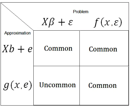
Of course, prediction itself can be divided into different types of predictors. Given a particular a
problem we may approach the modeling exercise as an approximation, where this approximation
may be some linear function, sayxβ+ǫ, or some nonlinear functionf(x, ǫ).
Let us now be more specific about how the prediction problem is formulated, given the
gen-eral, mean zero, stochastic processyt=f(Yt−1, ǫt), where againYt−1 represents the information
set generated by the stochastic process at timet−1.
It can be shown that in the general case, the optimal predictoryˆt|t−1 =f(Yt−1)under the
min-imum mean squared error (MMSE) criterion is the conditional expectation,E[yt|Yt−1]. That is,
the argmin of the quadratic loss function, the expected mean squared errorE(yt−f(Yt−1))2
Figure 3: Types of model approximations
can be shown to bef(Yt−1) = E[yt|Yt−1]. See see Priestley (1981, pg. 76) or Hamilton (1994,
pg. 72) for proof.
However, suppose instead that we wish to restrict our choice to the class oflinearpredictors.
That is,yˆt|t−1 = f(Yt−1) = a′y∗t−1 whereyt−∗ 1 =
yt−1 yt−2 yt−3 . . . y0
′
. Interestingly,
the value ofa′that satisfiesE yt−a′y∗t−1
y∗t−′1=0′, that is exhibits zero covariance between
forecast error and the independent variable, also minimizes the quadratic loss function above,
given the constraint of having to choose amongst linear predictors.
We call this value ofathelinear projection:
a′ =E[yty∗t−′1]E[y∗t−1y∗t−′1]−1, (63)
and the definition becomes clear when we note that:
f(Yt−1) = a′y∗t−1 =E[yty∗
′
t−1]E[y∗t−1y∗
′
t−1]−1y∗t−1 ≡ P[yt|Yt−1] (64)
and so P[yt|Yt−1] represents the scalar projection of yt onto the Hilbert space spanned by the
columny∗
Interestingly, if we consider the special case of the linear, Gaussian, stochastic process with
uncorrelated innovations, it turns out that the linear projection is equal to the conditional
expec-tation since we know that for Gaussian random variables:
E[yt|Yt−1] =Cov(yt, Yt−1)Cov(Yt−1, Yt−1)−1Yt−1
≡ P[yt|Yt−1], (65a)
which is a standard result involving partitioning the set Ytinto yt andYt−1, and without loss of
generality we assume all the elements ofYtare mean zero.
However, if the model is not linear in the stochastic variables, or if the stochastic processes
are neither weak white nor Gaussian, then there is no reason to believe that the linear projection
will prove the best predictor, although it is best amongst the class of linear predictors so that
M SE(P[yt|Yt−1])≥ M SE(E[yt|Yt−1]). This is because the linear projection is a function only
of the second moment properties of the stochastic processes.
Therefore, to summarize, we have three types of predictors (where one is a special case of the
other):
◦ The linear projection, P[yt|Yτ] τ ∈ {1, . . . , T}, which is some linear function of the
information set.
◦ The expectation,E[yt|Yτ], which may possibly be a nonlinear function of the information
set.
◦ The expectation under the assumption of a linear model and Gaussianity co-incides with
5.2
Examples
5.2.1 Prediction of VAR(1) process (weak form)
As a simple example, consider the case wherext, the state process in (1), is observed and that
the system matrices, including F, are time-invariant. That is, we assume that H = I and we
know the covariance matricesΣǫ >> 0andΣη =0. Therefore, the model is a VAR(1) and is a
special case of the state-space model in (1) – see equation (4a).
If the eigenvalues of F have modulus strictly less than 1, the VAR(1) can be inverted and
written as an VMA(∞):
xt =F xt−1+ǫt (66a)
= [I −FL]−1ǫt
=ǫt+F ǫt−1+F2ǫt−2 +. . . (66b)
Therefore, we can consider the stochastic process as being a linear function of weak white
noise,ǫt. That is, the information set is equivalently written asYt≡ {ǫt,ǫt−1, . . .}.
Now, we would like to try and predict xt conditional on information set Yt−1 under the
MMSE (minimum mean squared error) criterion. Let f(Yt−1) represent our predictor
func-tion. We would like to minimize a quadratic loss function, the expected mean squared error
E(xt−f(Yt−1)) (xt−f(Yt−1))′
, where f(Yt−1) is now a linear function of the information
set at timet−1. The “best” (in the sense of using the information embodied in the information set efficiently, according to the MMSE criterion), linear, predictor of the VAR(1) processxt, given
information setYt, is thelinear projection, defined asP[xt|Yt−1]≡xt|t−ˆ 1.
However, it is clear that the linear projection must be:
ˆ
since we have that:
E[(yt−xt|t−ˆ 1)x∗
′
t−1] =0 (68)
and from the discussion of the previous section we know that this value ofxtˆ−1 =f(Yt−1)must
be the argmin of the expected mean squared forecast error.
Note that we can also explicity solve for the value of a just as was done before, and this
provides a moment condition that can be used to alsoestimatethe system matrixF given sample
data by employing the sample moment counterpart,ˆa. Rewrite the model in (66b) as:
xt=ǫt+
F F2 . . .FQ
ǫt−1
ǫt−2
.. .
ǫt−Q
(69a)
=ǫt+A′ǫ∗t−1, (69b)
where we have truncated the lags atQ. We can therefore solve forA′ as:
xt=ǫt+A′ǫ∗t−1
⇔xtǫ∗t−′1 =ǫtǫ∗t−′1+A′ǫ∗t−1ǫ∗t−′1
⇔E[xtǫ∗ ′
t−1] =E[ǫtǫ∗ ′
t−1] +A′E[ǫ∗t−1ǫ∗
′ t−1]
⇔A′ =E[xtǫ∗ ′
t−1]E[ǫ∗t−1ǫ∗
′
t−1]−1. (70a)
esti-mate the population moment condition above via the sample averages: 1 T ′ X τ=1
xτǫ∗ ′
τ−1 →P E[xtǫ∗ ′
t−1], (71a)
and 1
T
′ X
τ=1
ǫ∗τ−1ǫ∗τ′−1 →P E[ǫ∗t−1ǫ∗t−′1]. (71b)
Finally, consider the case where the state process xt in (1) is in fact unobserved. 7 Now
we must also predict xt conditional on the information set Yτ (given different possible values
for τ). This is where the concepts of smoothing and filtering become important – we leave the discussion of prediction given unobserved state processes to Section 7 and the estimation of the
system matrices under these circumstances to Section 8 on estimation.
5.2.2 Prediction of static state-space model (strong form)
As another example, consider the case wherext, the state process in the strong form
state-space model (3), isunobservedand that the system matrices,F andH, and covariance matrices,
Σǫ andΣη are all time invariant. Moreover, in this case, the state process,xt, is i.i.d. Gaussian
and does not exhibit serial correlation. We call this model thestaticstate-space model and it is a
special case of the strong form model in (3) – see formula (28) above.
From the model in (28) we know that:
xt yt
=M V N
0 0 ,
Σǫ ΣǫH
′
HΣǫ HΣǫH′+Ση
. (72)
Moreover, from the discussion above, we know that given the linear Gaussian setting, the
linear projection is equivalent to conditional expectation. Therefore, the best linear predictors of
7
both observed and unobserved processes are given as:
E[yt|Yt−1] =HE[xt|Yt−1] +0=0, (73a)
and E[xt|Yt−1] =0. (73b)
However consider that the expectation of the state variable, conditional on current time t infor-mation, is not trivial:
E[xt|Yt] =E[xty′t]E[yty′t]−1yt (74a)
=E[xt(Hxt+ηt)
′
] [HΣǫH′+Ση]
−1
yt (74b)
=ΣǫH′[HΣǫH′+Ση]−1yt. (74c)
Note the difference between this example and that given in Section 5.2.1. In the previous case
the state processxtwasobservable, and so our prediction formula was really a prediction of the
observation process. However, in this case it is not.
Therefore we are confronted with two problems: a) predict future values of the observed
pro-cessytgiven information set Yt−1 and also b) predict the state process xt given the information
setYτ whereτ can range across different values. Ifτ =t, we call this the filtering problem and
if τ > t we call this the smoothing problem. Under the static model framework, the solution is simple. It is simply the linear projection P[xt|Yτ] above. However, when the state process
is not static, the problem becomes much more involved and involves updating the linear
projec-tion given new informaprojec-tion. This is the essence of the Kalman filter and fixed point smoother
algorithms discussed in Section 7. In fact, the Kalman filter solutions below collapse to the
expressions above when the state process is static. For another example of a static state-space
5.2.3 Bayesian interpretation of the state-space model
Within the Bayesian context we can always interpret the state transition equation (1a) as defining
the dynamics of a prior distribution on the stochastic parameterxt. For example, from the linear
state-space model in Section 2.1.2, if we view the “signal”xtto be astochastic parameter, then
the model is more akin to a linear regression ofHtregressed onytbut where the slope coefficient
xtis allowed to follow an unobserved stochastic process.
Given this interpretation we can work with the probability density functions implied by the
respective model, to derive the posteriordensity p(xt|Yt), where Yt = {yt,yt−1, . . . ,y1}(the
posterior density is therefore the filtered density of the latent state, xt). This will be done by
appealing to Bayes theorem, and in the process we will make use of the prior densityp(xt|Yt−1)
and the likelihoodp(yt|xt), given observed valuesytand stochastic parameterxt.
First, using Bayes theorem it can be shown that the posterior distributionp(xt|Yt)is derived
as:
p(xt|Yt) =
p(xt, Yt)
p(Yt)
= p(xt,yt, Yt−1)
p(yt, Yt−1)
where p(xt,yt, Yt−1) =p(yt|xt, Yt−1)p(xt|Yt−1)p(Yt−1)
=p(yt|xt)p(xt|Yt−1)p(Yt−1)
⇔p(xt|Yt) =
p(yt|xt)p(xt|Yt−1)
p(yt|Yt−1)
∝p(yt|xt)p(xt|Yt−1) (75a)
inno-vations,ǫtandηt, we have that the prior density is defined as:
p(xt|Yt−1)∼M V N(xˆt|t−1,Pt|t−1) (76a)
where xtˆ|t−1 =Fxtˆ−1|t−1 (76b)
and Pt|t−1 =F Pt−1|t−1F′ +Σǫ, (76c)
which follows directly from the linear projection of F xt−1 +ǫt into the space spanned byYt−1
[see (89a) and (100a) below]. Therefore, xˆt|t−1 is the forecast of the state variable xt, given
information at timet−1, which is a linear function ofxˆt−1|t−1, the filtered state variable.
Moreover, the likelihood given observed valuesytis given as:
p(yt|xt)∼M V N(Hxt,Ση) (77)
which follows immediately from the definition of the state-space model in (1). Therefore, given
the linear model, we have that the forecast ofytconditional on timet−1information is therefore
Hxˆt|t−1, which again follows from the linear projection.
Furthermore, by standard results on the moments of the product of two normal densities, we
have that the posterior distribution is proportional to:
p(xt|Yt)∼M V N(xˆt|t,Pt|t) (78a)
where xtˆ|t=Pt|t
P−t|t1−1xtˆ|t−1+H′Ση−1yt
(78b)
and Pt|t=
h
H′Ση−1H+P−t|t1−1
i−1
(78c)
where it can be shown that (78b) and (78c) are equal to (98b) and (100b), respectively. Therefore,
the above expressions provide a recursive system of equations that together generate the filtered
prediction of the state variable xtˆ|t [to see this sub (76b) into (78b) and (76c) into (78c)]. This
set of recursions is effectively the Kalman filter (1960) and so we can see that from the Bayesian
Gaussian innovations.
However, if the model is nonlinear we cannot expect the conditional expectation to be of a
linear form. Generally, we must approximate the set of filter recursions by numerical methods
such as Monte-Carlo. Essentially, we are able to generate the expectation of the filtered state
density in (75a) by drawing from it and appealing to a law of large numbers.
Harrison and Stevens (1976) presents the general discussion of the Bayesian approach to
state-space modeling.
6
Prediction in the frequency domain
Consider the engineering context, where the classical approach to linear time invariant
sys-tem analysis involved spectral representations and “frequency response” to unit shocks passed
through appropriate physical filters, the state, xt, has kept its interpretation as the “signal”
cor-rupted by noise. Since the signal is latent, we often wish to “extract” the signal from the noise
and this defines the “signal extraction” problem:
argmin{aj}∞
j=0E[(xt−xˆt)
2]
(79a)
where xˆt=
∞ X
j=0
ajyt−j, (79b)
and yt =xt+ηt, (79c)
and where ηtis a weak white noise, and we only observe the noisey signal yt. Moreover,xt is
uncorrelated with the noiseηt, and both processes are stationary. That is, we wish to “filter” out
the noise,ηt, to recover the signal,xt, when we only observe,yt. Under the MMSE criterion, the
optimal solution will minimize (79a), by choosing the sequence of filter coefficients{aj}∞j=0.
That is, given observations of the outputYt = {yt, yt−1, yt−2, . . .}, we wish to find the most
efficient predictor of the latent variablextin the sense of the discussion provided above in Section
mid-part of the last century. This solution is interpreted in terms of an optimaltransfer function,
A(e−iω), which is the Fourier transform of the impulse response function,{a j}∞j=0:
A(e−iω) = hxy(ω)
hyy(ω)
= hxx(ω)
hxx(ω) +hηη(ω)
(80a)
where A(z) =
∞ X
j=−∞
ajzj, (80b)
and where hxy(ω) is the cross-spectral density between xt and yt, and hxx(ω) is the spectral
density of xt. Therefore, we can see that the Wiener filter solution allows frequencies to pass
through when the signal-to-noise ratio is high, and vice versa when low:
hˆxˆx =|A(e−iω)|2hyy(ω). (81)
See Priestley (1981), Chapter 10, for more details.
However, given the advent of digital computers, the more useful time domain counterpart is
found in the work of Kalman (1960) and is discussed in more detail within Section 7.
Subsequently, the application of signal extraction methods to modern economics, and
empir-ical time-series analysis more generally, was developed by Nerlove et al. (1979) and popularized
by Harvey (1984,89) and the “Unobserved Components” framework which is discussed in
Sec-tion 9.4 (see also example 2.2.10).
7
Prediction in the time domain
Let us turn now to the general solutions of the following prediction problems in the time domain,
when the state-space representation is constrained to be linear:
1. Forecasting future values of yT+h for some horizon h given observed values from t = 1, . . . , T, or forecastingxT+h given predictions of the statexˆt|t, t= 1, . . . , T.