Impact of environmental dynamics on
economic evolution: A stylized
agent-based policy analysis
Nannen, Volker and van den Bergh, Jeroen C. J. M. and
Eiben, A. E.
IFISC, Institute for Cross-Disciplinary Physics and Complex
Systems, Universitat de les Illes Balears, Spain, ICREA, Barcelona,
Spain, Institute of Environmental Science and Technology,
Universitat Autònoma de Barcelona, Spain, Dept. of Economics and
Economic History, Universitat Autònoma de Barcelona, Spain,
Faculty of Economics and Business Administration, VU University
Amsterdam, the Netherlands, Institute for Environmental Studies,
VU University Amsterdam, the Netherlands, Department of
2013
Online at
https://mpra.ub.uni-muenchen.de/43673/
A stylized agent-based policy analysis
Volker Nannen∗
IFISC, Institute for Cross-Disciplinary Physics and Complex Systems, Universitat de les Illes Balears, 07122 Palma de Mallorca, Spain Departament d’Arquitectura i Tecnologia de Computadors, Universitat de Girona, Edifici P-IV, Campus de Montilivi, 17071 Girona, Spain
Jeroen C.J.M. van den Bergh
ICREA, Barcelona, Spain
Institute of Environmental Science and Technology, Universitat Autònoma de Barcelona, Edifici Cn, 08193, Bellaterra, Spain Dept. of Economics and Economic History, Universitat Autònoma de Barcelona, Edifici Cn, 08193, Bellaterra, Spain
Faculty of Economics and Business Administration, VU University Amsterdam, De Boelelaan 1105, 1081 HV Amsterdam, the Netherlands Institute for Environmental Studies, VU University Amsterdam, De Boelelaan 1105, 1081 HV Amsterdam, the Netherlands
A.E. Eiben
Department of Computer Science, Faculty of Sciences, VU University Amsterdam, De Boelelaan 1081a, 1081 HV Amsterdam, the Netherlands
Abstract
The general problem of how environmental dynamics affect the behavioral interaction in an evolutionary econ-omy is considered. To this end, a basic model of a dynamic multi-sector econecon-omy is developed where the evolution of investment strategies depends on the diversity of these strategies, social connectivity, and relative contribution of sector specific investments to production. Four types of environmental dynamics are examined that differ in how gradual and how frequently the environment changes. Numerical analysis shows how the socially optimal level of diversity increases with the frequency and speed of environmental change. When there is uncertainty about the specific type of environmental dynamics—whether for lack of data or because it is not constant—the socially optimal level of diversity increases with the degree of risk aversion of the policy maker or the society.
Keywords: agent-based economics, dynamic environments, evolutionary economics, optimal diversity, public policies, risk aversion
1. Introduction
1.1. Economic evolution in dynamic environments
Evolutionary reasoning and agent-based modeling have become standard practice in various disciplines, in-cluding social sciences [e.g.,1,2]. An evolutionary model uses a population of entities that undergo selection and variation. Although specific domains ask for the development of particular types of model, several common, gen-eral issues arise. Here we aim to address one such issue, namely, how environmental dynamics bears upon the behavioral interaction of an evolutionary economy consisting of multiple agents with heterogeneous economic
∗Corresponding author at: Departament d’Arquitectura i Tecnologia de Computadors, Universitat de Girona, Edifici P-IV, Campus de
Mon-tilivi, 17071 Girona, Spain.
Email addresses:[email protected](Volker Nannen),[email protected](Jeroen C.J.M. van den Bergh),[email protected]
(A.E. Eiben)
agent-strategies. Specifically, we will study whether different types of environmental dynamics call for distinct behav-ioral interaction, and how a policy maker can make use of this insight even when the current type of environmen-tal dynamics is unknown. The relevance of these questions is evident: few economic environments are static, and their dynamics are often irregular and unpredictable.
Generally, one cannot expect evolution in a changing environment to approach a steady state. Often, what matters is not how well the agents adapt if given enough time, but how fast they adapt to a new challenge. In a socio-economic context a wide range of environmental variables can be identified: macroeconomic condi-tions, technological opportunities, policies and institucondi-tions, and natural resources. When heterogeneous groups of users, polluters, or harvesting strategies are involved, a reduction to a representative agent model is often not possible. Instead, the heterogeneity and interaction of agents and strategies is better treated by an evolutionary agent-based model [3,4].
With regard to the evolutionary system, there is a range of theoretical starting points and modeling approaches [5,6]. First of all, one can choose to use very theoretical, abstract models of the evolutionary game type. In evolu-tionary game theory, studies of social behavior have been mostly limited to constant environments, letting selec-tion pressure depend on the populaselec-tion distribuselec-tion. This simplificaselec-tion allows for analytical treatment. However, addition of a dynamic environment typically leads to a system that is no longer amenable to analytic solutions. Numeric simulations of multi-agent systems form an alternative to the analytic approach that offers much more flexibility in examining system behavior. They allow a distinction between local and global environments, and be-tween stationary and mobile agents. They further allow to study the influence of population size, and the effects of dynamic environments on group and network formation [7,8]. In addition, different assumptions can be made re-garding selection factors and innovation mechanisms (random mutations, deterministic trends, recombination) and bounded rationality of agents (habits, imitation).
For our purpose a relevant distinction is between external and internal environmental dynamics. Whereas systems with only exogenous variables are relatively simple, endogenous variables generate complex feedback systems. Unfortunately, most real-world systems studied by biologists and social scientists are of the latter type. Yaari et al. [9] use local positive feedback loops to model growth in post-liberalized Eastern Europe. Implications of such a model to policy control are discussed by Challet et al. [10]. Ietri and Lamieri [11] and Windrum and Birchen-hall [12] model coevolution of consumers and firms to study product innovation, technological successions, and the emergence of business cycles. Resource dynamics [e.g.,13,14] and dynamic control of a pest population that evolves resistance to pesticides [15] are policy-relevant examples. Another, general example is a coevolutionary system in which two heterogeneous populations cause selection pressure on one another [16]. This leads to very complex coevolutionary interactions because the environment of each evolutionary (sub)system is evolving as well. Coevolution thus implies a particular type of internal environmental dynamics [17]. However, coevolution of multiple, interacting evolving populations easily leads to intractable models, and therefore is not a logical start-ing point for the present analysis (it may be addressed in a subsequent paper). We want to first know how a sstart-ingle population evolves under various types of environmental dynamics.
In this article we investigate the impact of different types of general external environmental dynamics on the socially optimal type of behavioral interactions among the agents in the population. For this purpose we de-velop a stylized, abstract evolutionary agent-based model that would best describe a community of small and medium-sized enterprises which serve similar markets with similar products, and which are characterized more by cooperation and an open exchange of information than by competition and secrecy. We identify the key control variable and establish its optimal level under different environmental dynamics and for different degrees of risk aversion of the policy maker or the society. While our results are solid insofar as they are robust over a wide range of implementation choices and parameter values, specific application would require adaptation of the model, for example, by including competition, niches, savings behavior, or coevolution of multiple populations.
Within economics, a quantitative approach with focus on control is more typical of the management literature. Here, the problem of how firms have to diversify and reinvent themselves in the face of various types of environ-mental dynamics is ubiquitous. While normally not phrased in evolutionary terms, the reader will agree that the essential elements of an evolutionary process—a population that undergoes variation and selection—are usually well defined. For example, Ansoff [23] and Ansoff et al. [24] conclude that a firm needs to diversify its portfolio of methods and products in order to stay profitable in a changing environment, and that the level of diversification— ranging in qualitative terms from “incremental” to “creative”—needs to match the degree of changeability and predictability of the environmental dynamics. Thore et al. [25,26] use data envelope analysis (DEA) to track the time path of the empirical production frontier for the U.S. computer industry. They observe that individual firms left the efficiency frontier and returned to it in accordance with the life cycles of their products and technologies. Building on this, Phillips and Tuladhar [27] show that the number of years a computer manufacturer stayed at the efficiency frontier corresponds to the amount by which it could adjust output levels to environmental stimuli. The authors proceed to link the optimal level of output flexibility to the variety of environmental stimuli, in accordance with the law of requisite variety [28].
1.2. A model of environmental change
Economic change in general and business cycles in particular are often characterized by sustained co-movement of several variables and sectors. For example, Hornstein and Praschnik [29] study co-movement between produc-tion sectors, Croux et al. [30] study co-movement in the output of economic regions, and Forbes and Rigobon [31] study co-movement in stocks. We take account of this empirical stylized fact by defining economic dynam-ics as co-movement of two or more production coefficients of a non-aggregate Cobb-Douglas type multi-sector economy. The production coefficients can depend on an array of economic dynamics, like technological develop-ment and resource dynamics. When the technology or the environdevelop-ment changes, the production coefficients can change as well.
Water management provides a specific example of a production input that is highly dependent on environ-mental conditions, available technology and the specific requirements of currently profitable crops. An example of global scale is the progressive desertification of farm land, which increases the dependency of farmers on irriga-tion. Specific local examples are provided by the Netherlands and South India. Since more than a millennium the already high Dutch water table has been rising even further due to soil compaction and the reduction of swamp areas that buffer excess surface water [32]. In response, the Dutch have learned to control the water table with a complex system of dikes, channels and water pumps of increasing cost and sophistication. South India is largely semi-arid. Most of its large rivers and tributaries are non-perennial. Originally, crops that depend entirely on rain fall and stored moisture in the soil were dominant. However, during the last millennium, and particularly during the Vijayanagara period (14t hto 17t hcentury), consumer preferences for wet rice and other irrigated crops stim-ulated heavy investment in a complex network of reservoirs, ponds, and irrigation canals [33]. These examples can be modeled as a gradual increase, possibly from zero, of the production coefficient of water management. Increased investment in water management necessarily reduces the relative importance of all other inputs, i.e., lowering the absolute value of their coefficient after normalization.
be rather inefficient. This inefficiency seems to be more pronounced in Bangladesh, where maize was introduced comparatively recently. An interpretation offered by the model developed here is that the maize producers of each region had previously optimized their investment behavior under different technological or environmental con-ditions, or for different crops, and that current dominant investment strategies are transitional, reflecting the fact that each group of producers is in the process of evolving their investment strategy from the previous optimal to the current optimal strategy.
1.3. Public policy and the evolution of economic behavior
In the present model agents have individual investment strategies that specify how they invest their respective income. Their objective is to maximize their individual welfare. Agents prefer investment strategies which give high welfare. Their rational capabilities are bounded and their information is limited. The only information avail-able to the agents is the investment strategies and the welfare of their fellow agents. The behavioral interactions influence how the agents use this information to evolve their investment strategies through imitation. Our frame-work postulates that the environmental dynamics are beyond the control of the policy maker, while he or she can regulate (some aspects of ) the agent interactions.
We assume that when an agent imitates, it tries to do so faithfully. Here, agents imitate investment portfolios, and how closely the original is matched depends on the accuracy of information on the original. Control over the accuracy of this information is a powerful policy instrument. For example, laws regarding the quality, frequency, and accessibility of balance sheet information of public companies were one of the major responses to the crisis of 1929, in this case to minimize the error made by investors. Yet for the vast majority of firms and countries, balance sheets are either not public, or are not of a quality that allows ready identification of the investment strategy. So the output (product) may be known but not the input. Other examples of policy tools that facilitate knowledge transfer between firms are sponsorship of trade fares, scientific venues, scholarships, and educative publications. By regulating how accurately agents can imitate each other, a policy maker can control the diversity of strate-gies within the population. We will study the effect of diversity on population welfare numerically through com-puter simulations. We will address two research questions. The first is whether different types of environmental dynamics call for distinct levels of diversity for the agents to achieve a high welfare. If this is the case, then it would be advantageous for a policy maker to first identify the specific type of environmental dynamics and, if identifica-tion is possible, to steer the level of diversity of strategies such that it would be optimal for that type of dynamics. The second question follows from the fact that the policy maker is often uncertain about the environmental dy-namics, either for lack of data, or because the dynamics is inherently irregular and unpredictable. This raises the issue of adequate policies under uncertainty: how do agent interactions that work well for one type of environ-mental dynamics perform under another environenviron-mental dynamics? Depending on the degree of risk aversion of the policy maker or the society, different policies can be recommended.
As for the environmental dynamics, we focus on two general aspects of environmental change: how fast it oc-curs, and how often, similar to the work of Ciarli et al. [36]. Speed and frequency of change are two aspects of an environmental dynamics that can relatively easily be observed and recognized. Depletion of a mineral resource, for example, typically manifests itself over an extended period of time, while a biotic resource like fish can disap-pear literally overnight. And a remote agricultural community is normally exposed to environmental hazards less frequently than one surrounded by a heavily industrialized region. If a policy maker can anticipate these aspects of environmental change, he or she might want to steer behavioral interaction such that economic agents can adapt well.
As has been extensively discussed by Wilhite [37], a study of economic interaction between social agents needs to give proper attention to the structure of the social network. Communication links between economic agents, whether individuals or organizations, are neither regular nor random. They are the result of a development pro-cess that is steered by, among others, geographic proximity, shared history, ethnic and religious affiliation, and common economic interests. Our simulations use a generic class of social networks that reproduce a number of stylized facts commonly found in real social networks. These are the small world property of Erd˝os and Renyi [38], the scale-free degree distribution of Barabási and Albert [39] and the high clustering coefficient of Watts and Strogatz [40].
relationship between an investment strategy and the generated income growth rate is studied. On the basis of this relation the environmental dynamics and the experimental setup are formulated in Section4. Section5provides simulation results and interpretations. Section6concludes.
2. The economic model
2.1. General features of the model
Consider a population of agents, each of which has the objective to reach a high level of individual welfare, something that can only be achieved through a sustained high income growth rate. Each agent can invest its re-spective income in a finite number of capital sectors. How it allocates its investment over these sectors is expressed by its individual investment strategy. Invested capital is non-malleable: once invested it cannot be transferred between sectors. Standard economic growth and production functions describe how the invested capital accu-mulates in each sector and contributes to income. These functions are not aggregated: growth and returns are calculated independently for each agent. Two agents with different investment strategies can experience different income growth rates and income levels.
The agents understand that there is a causal link between an investment strategy and economic performance as expressed by the income growth rate, but they cannot use calculus to find an investment strategy that maxi-mizes the income growth rate. Instead, the agents employ the smartest search method that nature has in store, evolution, and they evolve their investment strategies by imitation with variation. Since an agent prefers a high income growth rate over a low income growth rate, it imitates the investment strategy of a fellow agent when that fellow agent realizes an income growth rate that is high relative to its own income growth rate and the income growth rate of its other fellow agents. Imitation is not perfect. Changes that are introduced during imitation guar-antee diversity in the pool of strategies and keep the evolutionary search alive. In the terminology of evolutionary theory an agentselectsanother agent based on a property (thephenotype) that is indicative of its current economic performance and imitates its investment strategy (thegenotype) withvariation.
One can argue that the criterion for selection should not be the income growth rate, since income depends not only on the potential of the investment strategy, but also on savings behavior. More sophisticated criteria like the growth of returns on investments would indicate the potential of an investment strategy more accurately. Since the rationale for such criteria would be to avoid dependency of the evolution of investment portfolios on the savings behavior, we decided for a simple model without savings, so that the income growth rate is equal to the growth of returns to investments. Furthermore, in this model there is no cost of shifting strategy. If there was, it would introduce a time lag between imitation of a strategy (the ‘genotype’) and its expression as income growth rate (the ‘phenotype’). This slows down the evolutionary process without changing the general results. A cost of adoption introduces at least one free parameter, which is why we decided not to include it in the present analysis. The evolutionary model was deliberately designed to be neutral to as many economic implementation choices as feasible, among them dependency on returns on scale. In this model, dependency of returns on scale can only affect the evolutionary process if it influences how income growth rate changes with a change in strategy. If it does, either large or small investors can express an improved strategy with a higher income growth rate and are more likely to be imitated. Such a bias does not depend in any way on the type of strategy, and is entirely absorbed in the noise terms of the evolutionary process. We choose constant returns for mathematical elegance, not the least because it allows us to normalize the production coefficients.
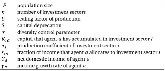
All variables and parameters of the economic model are summarized in Table1. For calibrated values of the free parameters, see Table3.
2.2. Strategies, investment, and production
The population approach means that accounting of capital investment, production, and income takes place at the level of individual agents. LetYa(t) be the income of agentaat timetand letnbe the number of available investment sectors. Formally, the investment strategysa(t) of an agent can be defined as ann-dimensional vector
sa(t)=[0, 1]n, X
i
Table 1:Variables and parameters of the model
|P| population size
n number of investment sectors β scaling factor of production δ capital deprecation σ diversity control parameter
Ki a capital that agentahas accumulated in investment sectori
πi production coefficient of investment sectori
si a fraction of income that agentaallocates to investment sectori Ya net domestic income of agenta
γa income growth rate of agenta
The partial strategysi a(t)—which is theit helement of a strategy—determines the fractionsi a(t)Ya(t−1) of income that agentainvests in sectori at timet. Each agent must invest its total income in one sector or another, so the partial strategies must be non-negative and sum to one. The set of all possible investment strategies is ann−1 dimensional simplex that is embedded inn-dimensional Euclidean space. We call this simplex the strategy space. Capital accumulation in each sector depends on the sector specific investment of each agent and on the global deprecation rateδ. Deprecation is assumed to be equal for all sectors and all agents. The dynamic equation for non-aggregate growth per sector is
Ki a(t)=si a(t)Ya(t−1)+(1−δ)Ki a(t−1). (2)
An extended version of this equation that accounts for dynamic prices can be found in the appendix. To calculate the incomeYa(t) from the capital that agentahas accumulated per sector, we use ann-factor Cobb-Douglas type production function with constant elasticity of substitution,
Ya(t)=βY
i
Ki a(t)πi(t), (3)
whereβis a scaling factor that controls the maximum possible income growth rate. The relative contribution of each sector to production is expressed by a dynamic vector of non-negative production coefficientsπ(t)= 〈π1(t) . . .πn(t)〉. To enforce constant returns to scale, all production coefficients are constraint to add up to one,
π(t)=[0, 1]n, X
i
πi(t)=1. (4)
Similar to the strategy space, the set of all possible vectors of production coefficients is ann−1 dimensional simplex that is embedded inn-dimensional Euclidean space. As explained in the introduction and because of the conclusions reached in Section3, we model the environmental dynamics as externally defined co-movement of two or more production coefficientsπ(t). This is a general approach that can also be applied to other economic dynamics such as technological development. Section4describes how we implement these changes and how we test whether or not they have an impact on behavioral interactions.
To measure how well a population of agents is adapted to a certain economic environment, we use the ex-pected log income E[logY(t)] of all agents at timet. Expected log income emphasizes an egalitarian distribution of income. Technically speaking, an economic agent with constant relative risk aversion prefers a society with high expected log growth and high expected log income. Let|P|be the total number of agents in the population P. We calculate expected log growth as
E[logY(t)]= 1 |P|
X
a
logYa(t). (5)
The individual income growth rateγa(t) is
γa(t)= Ya(t)
Expected log income relates to expected log income growth as
E[logY(t)]= t
X
i=1
E[log(γ(i)+1)]+E[logY(0)], (7)
where expected log income growth is defined as
E[log(γ(t)+1)]= 1 |P|
X
a
log(γa(t)+1). (8)
2.3. The evolutionary mechanism of behavioral interactions
From the point of view of evolutionary theory [22], agents and investment strategies are not the same: an agent carries or maintains a strategy, but it can change its strategy and we still consider it to be the same agent. Because every agent has exactly one strategy at a time, the number of active strategies is the same as the number of agents. The social structure of the agent population is modeled as a bi-directional network where the nodes are agents and the edges are communication links. Before the start of every simulation, a stochastic process assigns to each agentaa random set of peers that does not change during the course of the simulation. At each time steptof the simulation an agent may select one of its peers and imitate its strategy. That is, if agentais a peer of agentb, then acan imitateb, whilebcan imitatea. On the other hand, ifaandbare not peers, they can not imitate each other. For a detailed discussion of the network properties and its generation see [41].
The strategy of the imitating agent changes, while the strategy of the imitated agent does not. The choice of which agent to imitate is based on relative welfare as indicated by the current growth rate of income. The imitating agent always selects the peer with the highest current income growth rate. Only if an agent has no peer with an income growth rate higher than its own, the agent does not revise its strategy. If imitation was the only mechanism by which agents change their strategies, the strategies of agents that form a connected network must converge on a strategy that was present during the initial setup. However, real imitation is never without errors. Errors are called mutations in evolutionary theory. They are fundamental to an evolutionary process because they create and maintain the diversity on which selection can work.
In this model we implement mutation by adding some Gaussian noise to the imitation process. That is, when an agent imitates a strategy, it adds some random noise drawn from a Gaussian distribution with zero mean. This causes small mutations along each partial strategy to be more likely than large ones. The exact formula by which agentaimitates and then mutates the strategy of agentbis
sa(t)=sb(t−1)+N(0,σ), (9)
whereN(0,σ) denotes a normally distributedn-dimensional random vector with zero mean and standard
devia-tionσper dimension. Because partial investment strategies have to sum to one, we have to enforceN(0,σ)=0— for example by orthogonal projection of the Gaussian noise term onto the simplex—resulting in the loss of one degree of freedom. The error term is further constraint to leave all partial strategies positive. Needless to say that we do not imply that our boundedly rational agents engage consciously in such mathematical exercise. Subjec-tively they merely allocate their income such that none is left.
The sum of squares of thenpartial errors, i.e., the square of the Euclidean distance covered by the error, follows a chi-square distribution withn−1 degrees of freedom and mean (n−1)∗σ2. If all agents try to imitate the same optimal investment strategy of a static environment, the expected standard deviation of the partial strategies will in fact converge onσ. Since the parameterσcontrols the diversity of the investment strategies, we will call it the diversity control parameter, or simplydiversity. It is the only free parameter of this evolutionary mechanism and has potential policy implications. As has been shown by Nannen and Eiben [42], of the many parameters that can define an evolutionary process of imitation, calibration of diversity has the highest impact on agent welfare.
3. The evolutionary dynamics
3.1. The growth rate of a strategy
whether the strategy of an agent is imitated depends on whether the agent has a higher income growth rate than those agents it is compared to. We call the mapping from investment strategies to income growth rate thegrowth function. The growth function calculates the asymptotic growth rate that an imitating agent realizes if it holds on to a particular investment strategy. In the out-of-equilibrium system the actual income growth rate of an agent depends also on the investment strategy it was using before it adopted its current strategy. Dependency on the previous strategy constitutes a random factor to the income growth rate that is independent of the current strat-egy and that is therefore ignored in this analytical treatment. It is of course present in our out-of-equilibrium simulations.
If the growth function maps one strategy to a higher asymptotic growth rate than another strategy, then our evolutionary agents will prefer this strategy over the other strategy and imitate it. In this way the growth function indicates which of any two strategies will survive and propagate. Since it depends only on the order of income growth rates—i.e., which of any two agents has a higher income growth rate—whether an agent is imitated, the evolutionary dynamics is invariant under any strictly increasing transformation of the growth function. Any two growth functions that are strictly increasing (or decreasing) transformations of each other lead to the same evolu-tionary dynamics.
Let us start the derivation of the growth function with an analysis of the asymptotic ratio of sector specific capital to income,Ki a(t)/Ya(t), that will be achieved if an agent holds on to a particular strategy. The dynamic equation of this ratio is
Ki a(t) Ya(t) =
si a(t)Ya(t−1)+(1−δ)Ki a(t−1) (γa(t)+1)Ya(t−1)
= si a(t) γa(t)+1+
1−δ γa(t)+1
Ki a(t−1) Ya(t−1).
(10)
This equation is of the form
x(t)=a+bx(t−1), (11)
which under the condition 0≤b<1 converges monotonically to a limit at
lim
t→∞x(t)=a/(1−b). (12)
This condition is fulfilled here: investment is always non-negative and sector specific capital cannot decrease faster thanδ. With constant returns to scale, income cannot decline faster than capital deprecation, and we have γa≥ −δ. For the moment, let us exclude the special caseγa= −δ. Then, considering that 0<δ≤1, we have the required constraint
0≤ 1−δ
γa(t)+1<1 (13)
and we conclude that the ratio of capital to income converges to
lim t→∞
Ki a(t) Ya(t) =tlim→∞
si a(t) γa(t)+1/
µ
1− 1−δ γa(t)+1
=lim t→∞
si a(t) γa(t)+δ.
(14)
Equation14describes the limit ratio of sector specific capital to income to which the economy of an agent con-verges monotonically. We ignore the limit notation and combine equation14with equation3to calculate asymp-totic income as
Ya(t)=βY
i
µsi a(t)Ya(t)
γa(t)+δ
¶πi(t)
=β Ya(t) γa(t)+δ
Y
i
si a(t)πi(t).
We can now solve forγa(t) to derive the growth function
γa(t)=βY
i
si a(t)πi(t)−δ. (16)
Let us return to the special caseγa= −δ. According to equation2, capital per sector decreases at the depre-cation rateδonly when it receives zero investment, and it cannot decrease faster. This implies that with constant elasticity of substitution, a growth ofγa= −δis only possible if every sector with a positive production coefficient receives zero investment. This impliessi a(t)=0 for at least one partial strategy, and so equation16holds also for the special caseγa= −δ.
3.2. Efficiency and level sets of investment strategies
How does the income growth rate of an imitating agent compare to the income growth rate of a rational agent with perfect information? The termQ
isi a(t)πi(t)has a single optimum atsa(t)=π(t), allowing for a maximum growth rate of
γopt(t)=βY i
πi(t)πi(t)−δ. (17)
This is the income growth rate that a rational agent with perfect information would expect to achieve. Its exact value depends on the location of the production coefficients in the simplex. In ann-factor economy the term
Q
iπi(t)πi(t)varies between a value of 1/nin the center of the simplex where all production coefficients are equal, and a value of one in the corners of the simplex where one sector dominates. In order to remove this variability from the growth function, and to allow an easy comparison with the income growth rate of a rational agent with perfect information, we define the efficiencyE(s,t) of a strategys(t),
E(s,t)=Y i
µ
si(t) πi(t)
¶πi(t)
. (18)
The efficiency of a strategy measures the fractionγa(t)/γopt(t) of optimal growth that an agent achieves with its current strategy on the current production coefficients, assuming thatδ=0. If one strategy leads to a higher asymptotic growth rate than another, it is also more efficient. This measure of efficiency is a monotonous transfor-mation of the growth function that preserves all infortransfor-mation on which agent imitates which other agent, removes the variability due to the location of the optimum on the simplex, and allows us to measures growth in terms of what a rational agent with perfect information would achieve.
Efficiency, like the asymptotic growth rate, is a monotonically decreasing function of the Euclidean distance between a strategy and the current production coefficients,|sa(t)−π(t)|. This function is not symmetric about the optimum; its slope varies with the direction from the optimum. Figure1shows how the average efficiency of a strategy decreases as its Euclidean distance to the optimum increases when strategies and production coefficients are chosen at random from the simplex. Note the inverse S-shape of the graphs. As the Euclidean distance tends to zero, the gradient approaches zero. This implies that when an evolutionary population of agents converges on the optimum, the differences in growth caused by a small amount of diversityσaround the optimal strategy are negligible.
A set of strategies each with identical asymptotic growth rate, sayγ′, is called a level set and forms a contour hypersurface in the strategy simplex. All strategies that are enveloped by this hypersurface have an asymptotic growth rate that is higher thanγ′. This inner set is convex [for a related proof see43] and according to equation16
satisfies
Y
i
si a(t)πi(t)≥γ
′+δ
β . (19)
An important level set isQ
two-factor economy
0
0.5
1
0
0.5
1
four-factor economy
0
0.5
1
0
0.5
1
ten-factor economy
0
0.5
1
[image:12.595.68.532.110.211.2]0
0.5
1
Figure 1:Average efficiency as a function of Euclidean distance to the optimum.Notes:Thex-axis shows the Euclidean distance, they-axis the corresponding average efficiency. Note the convex shape around the optima.
ten investment sectors. The probability tends to zero asδ/βapproaches one. For givenδ/β, the probability that the asymptotic growth rate of a random strategy is positive decreases as the number of investment sectors in-creases. What is true for a single optimum is also true for multiple optima: the larger the number of sectors over which agents have to spread their investments, the higher the pressure to be close to any given optimum, whether niche or global optimum.
The parametersδandβdetermine the asymptotic growth rate associated with a given hypersurface, as well as the minimum and maximum asymptotic growth rate that can be achieved with given production coefficients. δandβdefine monotonous transformations of the growth function that are irrelevant to the order of asymptotic growth rates, and which do not affect the location of the optimum nor the shape of level sets. In other words, in this type of model, environmental dynamics will affect the evolution of strategies only in so far as they are expressed as co-movement of two or more production coefficients. Moreover, the rate of convergence in equation14does not depend on the scaling factorβ. We will make use of this fact later on in the experimental design where we use a dynamicβfor normalization, significantly reducing the variability of the numeric results.
4. Experimental setup
4.1. The environmental dynamics
The previous section has shown how the growth function, up to a monotonous transformation, depends on the co-movement of two or more production coefficients of a Cobb-Douglas type multi-sector economy. When the production coefficients change with the environmental dynamics, strategies that have previously generated a positive income growth rate can now generate a negative income growth rate. Agents that have converged on a strategy that has previously resulted in a high income growth rate can see their income decline and need to adapt their strategies to the new production coefficients. How does the magnitude and duration of this decline depend on the type of environmental dynamics and on the behavioral interactions among the agents? To answer this question we model the environmental dynamics as externally defined changes inπ(t). That is, the environmental
two-factor economy
0 0.5 1
0 0.5 1
four-factor economy
0 0.5 1
0 0.5 1
ten-factor economy
0 0.5 1
0 0.5 1
[image:12.595.71.529.584.685.2]dynamics that change the production coefficients are the independent variable that the policy maker responds to. The parameters of the imitation mechanism are the dependent variables that the policy maker aims to regulate.
We focus on two aspects of environmental dynamics: how gradual the environment changes, and how fre-quently. In combination they define four types of environmental dynamics where the production coefficients change gradually and with low frequency, gradually and with high frequency, suddenly and with low frequency, and suddenly and with high frequency. We compare these with a static environment and a control systems with-out imitation. As discussed in Section3.2, when strategies evolve in a static environment, they are expected to converge on the optimum strategy, and welfare at the population level will be at its highest. On the other hand, without imitation and with strategies that are randomly distributed over the strategy space and that stay constant throughout the simulation, the income growth rate of most agents is most likely negative, irrespective of the envi-ronmental dynamics. Expected log income will decline and welfare at the population level will be at its lowest.
We consider the general case where a change in the production coefficients is defined as the replacement of one vector of production coefficients by another, with each vector drawn independently and at random from the uniform distribution over the simplexP
iπi(t)=1. Replacement is instant for a sudden change and by linear transition for a slow change. To give an example, a sudden change can be modeled by setting the production coef-ficients of a two-factor economy toπ= 〈.1, .9〉up until timet, and toπ= 〈.4, .6〉fromt+1 onwards. Such extreme changes are characteristic of industries that depend on unreliable resources, e.g., a biotic resource susceptible to climate change like forests or fish. Gradual change in this model reaches its final state at the end of a cycle. It is modeled by changingπfrom〈.1, 9〉at timetto〈.4, .6〉at timet+xlinearly overxsteps, such that
π(t+j)=(x−j)π(t)+jπ(t+x)
x , 0≤ j ≤x, (20)
where the conditionsP
iπi=1 andπi≥0 for alliare fulfilled at all times. Such gradual changes are characteristic of industries that depend on reliable resources, e.g., a mineral resource like iron or coal, where known reserves will typically last for decades if not centuries. They are also characteristic of technical change, or changes in human capital.
As for the frequency of change, we model low frequency changes by starting the transition from one vector of production coefficients to another vector every fifty years, reflecting a Kondratiev type of wave [44] that is charac-teristic of industries that are not a driving force of innovation and change only with the general shift in production methods, e.g., forestry. To model high frequency changes the transition starts every ten years, corresponding to the fast business cycles observed by Juglar [45]. Such frequent changes are characteristic of industries that invest heavily in research and development, e.g., telecommunications and biotechnology. Both the Kondratiev wave and the Juglar cycle are generally understood to be related to capital investment dynamics and technological restruc-turing, as opposed to a mere change in the employment of existing inventory, which is generally understood to be represented by the even shorter Kitchin cycle [46].
We do not claim that the waves and cycles observed by Kondratiev and Juglar are caused by external environ-mental dynamics. Indeed, Dosi et al. [47] present an evolutionary multi-agent model where business cycles are endogenous, driven by investment dynamics. We merely use the observations by Kondratiev and Juglar to define the longest and the shortest frequency pattern of investment dynamics that have actually been observed with a reasonable amount of certainty. That is, while we acknowledge that technological innovations are driven by re-search and development, we treat their effect on the production coefficients as external environmental dynamics that producers have to adapt to. Since the empirical evidence for our different types of environmental dynamics displays a significant amount of variability, we assume that the policy maker is often uncertain about the current type of environmental dynamics.
The imitation mechanism has one free parameter, the diversityσ, which we assume to be under control of the policy maker. From the point of view of the policy maker, the level of diversity is optimal in the presence of environmental dynamicsdwhen it maximizes the expected log income of each agent under this dynamics,
σopt(d)=argmax
σ E(logY(t)
|σ,d). (21)
In order to find this optimal level for different environmental dynamics we use repeated numerical simulations with varying levels ofσand measure the expected log income at the end of each simulation, using standard statis-tical methods to reduce variance. Having identified the levelσopt(d) at which the expected log income is highest under a given environmental dynamics, we proceed to formulate policy advice on the socially optimal level ofσ when there is uncertainty about the type of environmental dynamics. To do so we measure the expected log in-come that an optimal levelσopt(d) generates on those environmental dynamicsd′6=
dwhere it is not optimal. We then calculate the level that policy makers with various degrees of risk aversion assign to eachσopt(d).
4.2. Implementation details, model calibration, and scaling
The numerical simulations are based on a discrete synchronous time model where the income and strategy of each agent is updated in parallel at fixed time intervals. We consider each time steptto simulate one financial quarter. As no significant financial market requires a publicly traded company to publish financial results more than four times a year, we consider it the limit of feasibility to account for growth and to review an economic strategy as often as four times a year. Most economic agents will alter their strategy less often. Each simulation step is divided into two separate update operations:updating the economy—each agent invests its income according to its own investment strategy and the individual incomes and growth are calculated by the non-aggregate growth and production and growth functions—andupdating the strategies, when all agents compare their income growth rate with that of their peer group, and when those agents that decide to imitate change their respective strategies simultaneously.
Each computer simulation spans 500 time steps, simulating 500 financial quarters or 125 years. These are di-vided into an initialization phase of 100 time steps or 25 years, and a main experimental phase of 400 time steps or 100 years. An initialization phase is needed so that simulation results do not depend on the arbitrary choice of initial values. During initialization the simulated economy stabilizes and a “natural” distribution of strategies and growth emerges. Initial conditions are always defined in the same way: all strategies and the initial produc-tion coefficients are drawn independently at random from the simplex. The producproduc-tion coefficients are kept static throughout the initialization phase but the agents can imitate in the same way as they do during the main exper-imental phase, with the same diversityσ. During the 400 time steps (100 years) of the main experimental phase the agents have to adapt to the dynamic changes in the production coefficients. To avoid initialization effects, the increase in log income is measured from the beginning of the main experimental phase.
[image:14.595.191.405.673.732.2]Numerical methods are inherently constraint by the availability of computational resources. The computa-tional complexity of multi-agent systems typically scales at least polynomially with system size. The accepted method is to extensively study a system that is large enough to incorporate all the essential ingredients of the model, and to only increase the system size to test whether the obtained results are scalable. Here the main experiments are based on an economy of 200 agents and a four-factor economy. Sensitivity and scalability are tested with 1,000 agents and with a ten-factor economy. In order to understand whether the results depend on the specific implementation of the evolutionary mechanism, we also test more sophisticated implementations: one version where each agent imitates with probability .1 at every step—as opposed to probability one in the main
Table 2:The environmental dynamics used for numerical analysis Environmental dynamics Example
gradual, low frequency oil/gas reserves sudden, low frequency climate change
Sector 1
1 500
0
1 Sector 2
1 500
0
1 Sector 3
1 500
0
1 Sector 4
1 500 0 1 Area plot 1 500 0 1 Static environment Sector 1 1 500 0 1 Sector 2 1 500 0 1 Sector 3 1 500 0 1 Sector 4 1 500 0 1 Area plot 1 500 0 1
Gradual and low frequency dynamics
Sector 1 1 500 0 1 Sector 2 1 500 0 1 Sector 3 1 500 0 1 Sector 4 1 500 0 1 Area plot 1 500 0 1
Gradual and high frequency dynamics
Sector 1 1 500 0 1 Sector 2 1 500 0 1 Sector 3 1 500 0 1 Sector 4 1 500 0 1 Area plot 1 500 0 1
Sudden and low frequency dynamics
Sector 1 1 500 0 1 Sector 2 1 500 0 1 Sector 3 1 500 0 1 Sector 4 1 500 0 1 Area plot 1 500 0 1
[image:15.595.72.533.107.504.2]Sudden and high frequency dynamics
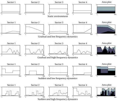
Figure 3:Environmental dynamics: changes in the production coefficients.Notes:Each row illustrates a different type of en-vironmental dynamics. The sequences of production coefficients are chosen at random. Thex-axis shows the 500 time steps (initialization and main experimental phase). They-axis of the four graphs positioned at the left of each row shows the value of one particular production coefficient in a four-factor economy. The single graphs at the right are area plots that visually combine the values of the same four production coefficients by stacking them one on top of the other, with a different shade of gray under each curve.
experiment—and one version where imitation is partial, such that a new strategy is a linear combination of the imitated strategy (with weight .1) and the strategy of the imitating agent (with weight .9). As before,σcontrols the standard deviation of the normally distributed errors per partial strategy.
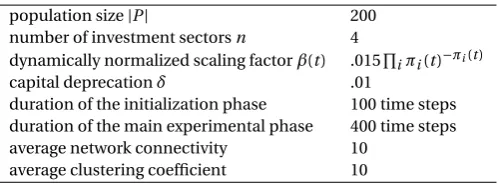
Table 3:Values of free simulation parameters population size|P| 200 number of investment sectorsn 4 dynamically normalized scaling factorβ(t) .015Q
iπi(t)−πi(t)
capital deprecationδ .01
duration of the initialization phase 100 time steps duration of the main experimental phase 400 time steps average network connectivity 10
average clustering coefficient 10
factorβ(t) depend on the vector of production coefficients,
β(t)=.015Y i
πi(t)−πi(t). (22)
With this normalization the asymptotic growth rate of all strategies is constraint to the range [-.01, .005], where the minimum of -.01 is realized whensi a(t)=0 for some positiveπi and where the maximum of .005 is realized whensa(t)=π(t). Numerical tests show that with these parameter values the probability that a random strategy has a negative asymptotic growth rate on random production coefficients is about .65. In other words, model parameters are calibrated such that two thirds of the strategy space has negative income growth. In the long run, agents can only experience positive income growth if they adapt.
To improve the general validity of our results we use large number of numerical simulations where—rather than closely calibrating those factors that affect the evolutionary dynamics on a specific economy—we define broad parameter ranges and collect statistical information over a representative sample of possible economies that fall within these ranges. For example, in order to obtain general results for specific environmental dynamics, each simulation uses an independent random sequences of production coefficients, which are replaced according to the speed and frequency of the respective environmental dynamics. Likewise, in order to obtain results that are valid for the general class of scale-free social networks with a high cluster coefficient, each simulation is based on an independent random instance of the social network. The generated networks have an average clustering coef-ficient1of .66 and an average connectivity of ten, meaning that the overall network can be subdivided into a few local clusters that maintain a high degree of internal connectivity, and a somewhat lower degree of connectivity to agents outside the respective cluster. The number of simulations needed to obtain reliable statistical results is determined by standard methods of variance reduction. The values of the free parameters used in the simulations are listed in Table3.
5. Results
5.1. Economic significance of diversity
Figure4shows the expected log income of an agent for varying levels of the diversity control parameterσ: for the control system without imitation, the static environment, and the four types of environmental dynamics. 50,000 simulations are used for each graph. 500 different levels ofσfrom the range [0, .5] are evaluated, and results are averaged over 100 simulations per level. The plots are smoothed with a moving average with a window size of ten levels.
In the first graph of Figure4—the control system without imitation—expected log income is uniformly nega-tive for all levels ofσ. This graph is based on a static environment, but the same is observed for any environmental dynamics. All other graphs of Figure4show systems with imitation and there is a clear functional relation between the level ofσand log income. For each system there is a single optimumσopt(d) that maximizes log income under
1In their seminal article Watts and Strogatz [40] define the clustering coefficient of a node as the number of all direct links between the
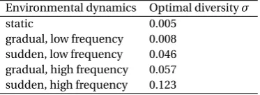
the given environmental dynamicsd. The exact values of the optima are given in Table4. The level ofσopt(d) is higher for more frequent changes than for less frequent changes, and higher for sudden changes than for gradual changes. Its level is lowest in the static environment. Further to this, the graphs show a clear pattern in the rela-tionship betweenσand expected log income: the slope to the left of the optima, i.e., for small levels ofσ, is much steeper than to the right, whereσis large. In other words, if agents tend to imitate faithfully, providing them with perfect information will not create the variation that is needed to adapt to change. We will revisit this fact in our discussion of policy advice under uncertainty.
Control system without imitation
0 0.1 0.2 0.3 0.4 0.5 -1
0 1 2
diversityσ
Static environment
0 0.1 0.2 0.3 0.4 0.5 -1
0 1 2
diversityσ
Gradual and low freq. dynamics
0 0.1 0.2 0.3 0.4 0.5 -1
0 1 2
diversityσ
Gradual and high freq. dynamics
0 0.1 0.2 0.3 0.4 0.5
-1 0 1 2
diversityσ
Sudden and low freq. dynamics
0 0.1 0.2 0.3 0.4 0.5 -1
0 1 2
diversityσ
Sudden and high freq. dynamics
0 0.1 0.2 0.3 0.4 0.5
-1 0 1 2
[image:17.595.62.524.207.427.2]diversityσ
Figure 4:Expected log income as a function of the diversity parameterσ.
Our first research question can now be answered: almost any level of diversityσwill allow the evolutionary agents to reach a positive income under any environmental dynamics, yet a unique optimum where income is highest can be identified for each environmental dynamics. So while it is not mandatory to define policies that effectσ, in the sense that imitating agents can almost always return to positive growth, it is optimal in the sense that there can be a significant gain in income.
5.2. Policy advice under uncertainty
The environmental dynamics does not need to be constant. And even when it is, the policy maker will often be uncertain about it for lack of data. In such cases of uncertainty the optimal diversityσdepends on the risk prefer-ence of the policy maker. We consider four types of risk preferprefer-ence: extreme risk seeking (maxmax), modest risk seeking (max average), modest risk aversion (minimax regret), and extreme risk aversion (maxmin). We calculate the optimal level for each preference from a generalization table where eachσthat is optimal under one environ-mental dynamics is applied to the other tested environenviron-mental dynamics, including the static environment. The
Table 4:Optimal level of diversityσfor a static environment and for each type of environmental dynamics Environmental dynamics Optimal diversityσ
[image:17.595.206.393.659.727.2]Table 5:Expected log income when a level of diversityσthat is optimal under one environmental dynamics is applied to other environmental dynamics
Environmental dynamics Environmental dynamics thatσwas optimized for thatσis applied to
Static Gradual, low freq. Sudden, low freq. Gradual, high freq. Sudden, high freq.
Static 1.996 1.995 1.95 1.93 1.79
Gradual, low freq. 1.988 1.991 1.97 1.96 1.88 Sudden, low freq. 1.12 1.25 1.412 1.406 1.33 Gradual, high freq. 0.55 0.72 1.38 1.39 1.31 Sudden, high freq. -0.04 0.09 0.53 0.55 0.60
Notes:Each column shows the expected log income when the level of diversity that is optimal for one type of environmental dynamics is applied to another type of environmental dynamics. Each row shows the expected log income when agents adapt to a specific environmental dynamics with a level of diversityσthat is optimal for another dynamics.
result is shown in Table5. Each entry shows the expected log income when a level of diversityσis applied to envi-ronmental dynamics different from the one where it is optimal. That is, each row shows the expected log income for the same environmental dynamics but differentσ, and each column shows results for the sameσbut different environmental dynamics. The log income of each entry is averaged over 10,000 simulations, where each simula-tion is based on a distinct instance of the social network and a distinct sequences of producsimula-tion coefficients. The values in the diagonal entries are highest for each row, confirming that the optimal level is indeed the best choice for a given environmental dynamics.
For each risk preference, each testedσcan now be associated with an expected log income value, and theσ with the best such value is considered optimal for the type of risk preference. This is shown in Table6. Each row shows the expected log income associated with eachσunder a given risk adversity, with the optimal expected log income in Italic type. A risk seeker looks at the highest expected log income that each testedσhas achieved under the different environmental dynamics, and chooses the highest of these. Risk neutrality means choosing theσ that maximizes the average expected log income over all environmental dynamics.
Often, policy makers are judged based on posterior knowledge. A minimax regret policy maker does not know the nature of the change, but knows that his critics will hold him accountable for the discrepancy between what could have been achieved if he had known, and what he actually achieved. So he minimizes this discrepancy [48]. Under minimax regret theσis chosen that minimizes the greatest possible difference between actual log income and the best log income that could have been achieved. Minimax regret first calculates the maximum possible regret for eachσand all environments, and then chooses theσthat minimizes this maximum. Risk aversion means choosing theσthat promises the highest minimum log income under any environmental dynamics.
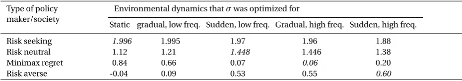
The numerical results clearly show that under uncertainty the optimal level ofσrises with the degree of risk aversion. This is in line with our earlier observation about the functional relationship between diversityσand
Table 6:Optimal policy advice under uncertainty and different degrees of risk aversion Type of policy Environmental dynamics thatσwas optimized for
maker/society
Static gradual, low freq. Sudden, low freq. Gradual, high freq. Sudden, high freq. Risk seeking 1.996 1.995 1.97 1.96 1.88 Risk neutral 1.12 1.21 1.448 1.446 1.38 Minimax regret 0.84 0.66 0.07 0.06 0.20 Risk averse -0.04 0.09 0.53 0.55 0.60
[image:18.595.64.530.603.685.2]expected log income: the gradient is steeper for lower levels ofσthan for higher levels, which makes higher levels ofσthe safer bet. These observations are confirmed by control experiments that test for sensitivity and scalability and that use alternative implementations of the imitation mechanism.
We also tested more sophisticated imitation mechanisms where either only a random selection of 10% of all agents would imitate per step, or where imitation was partial, such that a new strategy is a linear combination of the imitated strategy and the strategy of the imitating agent (again with normally distributed errors per partial strategy). We also made the selection process—the choice of which agent to imitate—dependent on income in-stead of growth. In all cases the arrangement of optimal levelsσopt(d) is similar for each environmental dynamics. The gradient is always steeper for small levels ofσthan for large ones. Under uncertainty the optimal level ofσ always increases with the degree of risk aversion.
5.3. Evolutionary dynamics
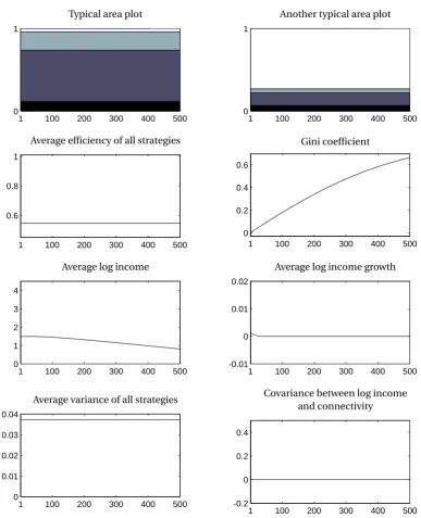
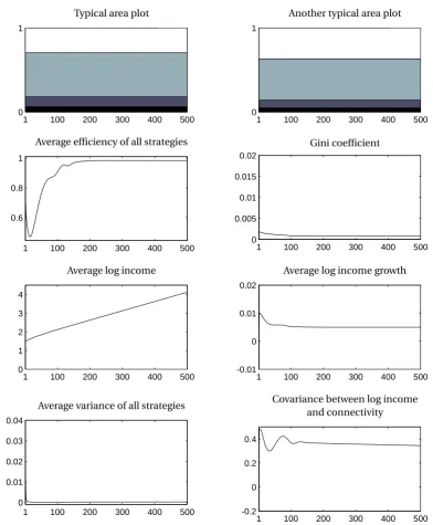
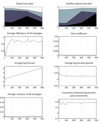
Figure5–10show the evolution of some key statistics during the 500 times steps of the simulation. Figure5 discusses the control systems without imitation (a static environment is used). Figure6discusses imitation in a static environment. The remaining four figures discuss the four types of environmental dynamics where changes occur gradually and with low frequency (Figure7), gradually and with high frequency (Figure8), suddenly and with low frequency (Figure9), and suddenly and with high frequency (Figure10). Each figure uses the optimal level of σfor the respective type of environmental dynamics (Table4). Figure4shows that that there is a fair degree of robustness for the optimal level ofσ. We evaluated the each type of environmental dynamics for all levels ofσ between zero and 0.5. The patterns shown in Figure5–10are representative for a wide range (±0.1) of sigma.
Each figure contains six statistics that describe the economic performance of the agent population, the het-erogeneity of their strategies, and the relevance of connectivity in the social network at each of the 500 time steps of the simulation. These statistics are averaged over 10,000 simulations. Each simulation uses a distinct instance of the social network and a distinct sequence of vectors of production coefficients. Two area plots on top of each group of six illustrate how the production coefficients change under the respective environmental dynamics. Each area plot shows a single distinct random sequence of production coefficients. To further ease the analysis, in Fig-ure7–10dotted vertical lines are inserted into each area plot and each of the six statistics to show the points in time where the transition to a new set of production coefficients starts.
All statistics react visibly to any change in the production coefficients. This is particularly interesting for those environmental dynamics where change occurs gradually, because when a new vector of random production co-efficients is introduced only the momentum changes, not the rate of change. And yet there is a clear and strong economic response to this change in momentum. Note that while we study an out-of-equilibrium system, many statistics have reached some sort of equilibrium after the 100 steps of the initialization phase.
Of the six statistics, the first four visualize the economic performance of the agents. The first statistic shows the average efficiency (see equation18) over all strategies, allowing a direct comparison to what rational agents with perfect information would achieve. The second statistic shows the behavior of the Gini coefficient, a measure of how egalitarian the accumulated capital is distributed. The third statistic shows average log income, which generally behaves as expected: after each change the income level drops temporarily, only to grow continuously thereafter. The fourth statistic shows average log growth, which falls dramatically immediately after a change, as most strategies become obsolete, but peaks within no less than ten time steps after the change, indicating that the recovery process of our evolutionary economy starts almost immediately after a change. The fifth statistic measures the variance of partial strategies within the population and shows how the heterogeneity of strategies is affected by a change in production coefficients. As discussed in Section2.3, in a static environment the square root of this variance approaches the level of the diversity control parameterσ. The sixth and final statistic measures the covariance between log income and connectivity, to emphasize the effect of a skewed distribution of connectivity on the evolutionary process. It shows how the correlation between log income and network connectivity rises each time that a new change in the production coefficients is initiated. Evidently the highly connected agents are among the first to learn and profit from the improved strategies.
Typical area plot
1 100 200 300 400 500
0 1
Another typical area plot
1 100 200 300 400 500
0 1
Average efficiency of all strategies
1 100 200 300 400 500
0.6 0.8 1
Gini coefficient
1 100 200 300 400 500
0 0.2 0.4 0.6
Average log income
1 100 200 300 400 500
0 1 2 3 4
Average log income growth
1 100 200 300 400 500
-0.01 0 0.01 0.02
Average variance of all strategies
1 100 200 300 400 500
0 0.01 0.02 0.03 0.04
Covariance between log income and connectivity
1 100 200 300 400 500
[image:20.595.113.501.102.580.2]-0.2 0 0.2 0.4
Figure 5:Average time evolution of an economy without imitation (the environment is static).Notes:The two area plots on top show single random sequences of production coefficients. The other statistics are averaged over 10,000 simulations. Thex-axis shows the 500 time steps while they-axis shows the respective statistics.
Typical area plot
1 100 200 300 400 500
0 1
Another typical area plot
1 100 200 300 400 500
0 1
Average efficiency of all strategies
1 100 200 300 400 500
0.6 0.8 1
Gini coefficient
1 100 200 300 400 500
0 0.005 0.01 0.015 0.02
Average log income
1 100 200 300 400 500
0 1 2 3 4
Average log income growth
1 100 200 300 400 500
-0.01 0 0.01 0.02
Average variance of all strategies
1 100 200 300 400 500
0 0.01 0.02 0.03 0.04
Covariance between log income and connectivity
1 100 200 300 400 500
[image:21.595.109.502.103.579.2]-0.2 0 0.2 0.4
Figure 6:Average time evolution of an economy and a static environment.Notes:The two area plots on top show single random sequences of production coefficients. The other statistics are averaged over 10,000 simulations. Thex-axis shows the 500 time steps while they-axis shows the respective statistics. Note how most statistics have stabilized during the first 100 steps of the initialization phase.
the environmental change. Finally, during the last phase of exploration, the agents seem to finally settle into the new order. Average efficiency increases again, and as more and more agents approach the (moving) optimum, they diversify around it.
Typical area plot
1 100 200 300 400 500
0 1
Another typical area plot
1 100 200 300 400 500
0 1
Average efficiency of all strategies
1 100 200 300 400 500
0.6 0.8 1
Gini coefficient
1 100 200 300 400 500
0 0.005 0.01 0.015 0.02
Average log income
1 100 200 300 400 500
0 1 2 3 4
Average log income growth
1 100 200 300 400 500
-0.01 0 0.01 0.02
Average variance of all strategies
1 100 200 300 400 500
0 0.01 0.02 0.03 0.04
Covariance between log income and connectivity
1 100 200 300 400 500
[image:22.595.114.501.101.580.2]-0.2 0 0.2 0.4
Figure 7:Average time evolution of an economy with imitation and a dynamic environment characterized by gradual, low fre-quency changes.Notes:The two area plots on top show single random sequences of production coefficients. The other statis-tics are averaged over 10,000 simulations. Thex-axis shows the 500 time steps while they-axis shows the respective statistics.
its investment portfolio, and the way a community of agents organizes itself around a dynamic optimum. When an agent changes its investment strategy, it will take some time until its growth rate has reached the corresponding income growth rate. The growth rate will approach the stable state always from above. This means that the income growth rate of an agent is highest immediately after the change, and then slowly diminishes until it has converged at the stable state that characterizes the strategy [49].
Typical area plot
1 100 200 300 400 500
0 1
Another typical area plot
1 100 200 300 400 500
0 1
Average efficiency of all strategies
1 100 200 300 400 500
0.6 0.8 1
Gini coefficient
1 100 200 300 400 500
0 0.005 0.01 0.015 0.02
Average log income
1 100 200 300 400 500
0 1 2 3 4
Average log income growth
1 100 200 300 400 500
-0.01 0 0.01 0.02
Average variance of all strategies
1 100 200 300 400 500
0 0.01 0.02 0.03 0.04
Covariance between log income and connectivity
1 100 200 300 400 500
[image:23.595.113.501.101.579.2]-0.2 0 0.2 0.4
Figure 8:Average time evolution of an economy with imitation and a dynamic environment characterized by gradual, high frequency changes. Notes:The two area plots on top show single random sequences of production coefficients. The other statistics are averaged over 10,000 simulations. Thex-axis shows the 500 time steps while they-axis shows the respective statistics.
Typical area plot
1 100 200 300 400 500
0 1
Another typical area plot
1 100 200 300 400 500
0 1
Average efficiency of all strategies
1 100 200 300 400 500
0.6 0.8 1
Gini coefficient
1 100 200 300 400 500
0 0.005 0.01 0.015 0.02
Average log income
1 100 200 300 400 500
0 1 2 3 4
Average log income growth
1 100 200 300 400 500
-0.01 0 0.01 0.02
Average variance of all strategies
1 100 200 300 400 500
0 0.01 0.02 0.03 0.04
Covariance between log income and connectivity
1 100 200 300 400 500
[image:24.595.113.501.102.580.2]-0.2 0 0.2 0.4
Figure 9:Average time evolution of an economy with imitation and a dynamic environment characterized by sudden, low fre-quency changes.Notes:The two area plots on top show single random sequences of production coefficients. The other statis-tics are averaged over 10,000 simulations. Thex-axis shows the 500 time steps while they-axis shows the respective statistics.
6. Summary
Typical area plot
1 100 200 300 400 500
0 1
Another typical area plot
1 100 200 300 400 500
0 1
Average efficiency of all strategies
1 100 200 300 400 500
0.6 0.8 1
Gini coefficient
1 100 200 300 400 500
0 0.005 0.01 0.015 0.02
Average log income
1 100 200 300 400 500
0 1 2 3 4
Average log income growth
1 100 200 300 400 500
-0.01 0 0.01 0.02
Average variance of all strategies
1 100 200 300 400 500
0 0.01 0.02 0.03 0.04
Covariance between log income and connectivity
1 100 200 300 400 500
[image:25.595.107.501.103.578.2]-0.2 0 0.2 0.4
Figure 10:Average time evolution of an economy with imitation and a dynamic environment characterized by sudden, high frequency changes. Notes:The two area plots on top show single random sequences of production coefficients. The other statistics are averaged over 10,000 simulations. Thex-axis shows the 500 time steps while they-axis shows the respective statistics.
has a clear policy dimension and policy makers might want to control the amount of information that agents have about the investment strategy of their peers. They can achieve this, for example, by giving access to balance sheets, or by extracting and publishing the investment strategy and economic performance.