Quantifying gaze and mouse interactions on
spatial visual interfaces with a new movement
analytics methodology
Ursˇka Demsˇar1☯*, Arzu C¸ o¨ ltekin2☯
1 School of Geography & Sustainable Development, University of St Andrews, St Andrews, Scotland, United
Kingdom, 2 Department of Geography, University of Zurich, Zurich, Switzerland
☯These authors contributed equally to this work.
Abstract
Eye movements provide insights into what people pay attention to, and therefore are com-monly included in a variety of human-computer interaction studies. Eye movement recording devices (eye trackers) produce gaze trajectories, that is, sequences of gaze location on the screen. Despite recent technological developments that enabled more affordable hardware, gaze data are still costly and time consuming to collect, therefore some propose using mouse movements instead. These are easy to collect automatically and on a large scale. If and how these two movement types are linked, however, is less clear and highly debated. We address this problem in two ways. First, we introduce a new movement analytics meth-odology to quantify the level of dynamic interaction between the gaze and the mouse pointer on the screen. Our method uses volumetric representation of movement, the space-time densities, which allows us to calculate interaction levels between two physically different types of movement. We describe the method and compare the results with existing dynamic interaction methods from movement ecology. The sensitivity to method parameters is evalu-ated on simulevalu-ated trajectories where we can control interaction levels. Second, we perform an experiment with eye and mouse tracking to generate real data with real levels of interac-tion, to apply and test our new methodology on a real case. Further, as our experiment tasks mimics route-tracing when using a map, it is more than a data collection exercise and it simultaneously allows us to investigate the actual connection between the eye and the mouse. We find that there seem to be natural coupling when eyes are not under conscious control, but that this coupling breaks down when instructed to move them intentionally. Based on these observations, we tentatively suggest that for natural tracing tasks, mouse tracking could potentially provide similar information as eye-tracking and therefore be used as a proxy for attention. However, more research is needed to confirm this.
a1111111111 a1111111111 a1111111111 a1111111111 a1111111111 OPEN ACCESS
Citation: Demsˇar U, C¸o¨ltekin A (2017) Quantifying gaze and mouse interactions on spatial visual interfaces with a new movement analytics methodology. PLoS ONE 12(8): e0181818.https:// doi.org/10.1371/journal.pone.0181818
Editor: Andrew Anderson, The University of Melbourne, AUSTRALIA
Received: July 13, 2016
Accepted: July 7, 2017
Published: August 4, 2017
Copyright:©2017 Demsˇar, C¸o¨ltekin. This is an open access article distributed under the terms of theCreative Commons Attribution License, which permits unrestricted use, distribution, and reproduction in any medium, provided the original author and source are credited.
Data Availability Statement: Data are provided as Supporting Information.
Funding: This research was supported by the Royal Society (https://royalsociety.org/) through an International Exchange Programme grant (IE120643) awarded to UD and AC¸. The funder had no role in study design, data collection and analysis, decision to publish, or preparation of the manuscript.
Introduction
Humans experience the world through a variety of senses, among which vision plays a domi-nant role [1,2]. Visual processes can be bottom-up (environmental features attract our atten-tion), or top-down (we consciously decide where to look); but in either case, human visual behaviour is often linked to attention [3]. Therefore, studying eye movements can reveal valu-able insights into how people think, especially when performing visuo-spatial tasks.
Eye movements are recorded using specialized eye tracking devices that register a series of gaze positions on a display. Through eye tracking, we obtain temporal sequences of gaze loca-tions, or the so-calledgaze trajectories. Raw gaze trajectory data are typically aggregated into
scanpaths, i.e., sequences of fixations (locations where eye is ‘fixed’ for a brief period of time) and saccades (quick movements between fixations) [4]. A number of methods have been pro-posed to analyse aggregated scanpaths (gaze plots, ‘heat maps’, methods to assess consistency of scanpaths, aggregation of scanpaths into areas of interest, etc., see [5] for a comprehensive review); however, the raw gaze trajectories, which represent the actual eyemovements, have been largely neglected.
In recent years, eye tracking devices are becoming more affordable [6] and new technologi-cal solutions appear to allow crowdsourcing eye tracking [7]. Nonetheless, eye tracking experi-ments are still complex, costly and time consuming, require dedicated devices, and despite the recent developments, currently, reliable eye movement data can only be collected one person at a time [8–10]. Therefore, as an alternative (or, in addition to eye tracking, especially those with lower accuracy such as web-cam based eye tracking without integrated active sensors), studying mouse movements has been suggested, as mouse movements can also express certain cognitive processes during visuo-spatial task solving [11]. Collecting mouse data has practical advantages as most devices are already equipped with a mouse (i.e. they not require additional specific equipment), and mouse data can be collected automatically as a background process for a large number of participants in parallel. Using mouse trajectories as a proxy for gaze tra-jectories has been proposed by Huang et al. [12], and various studies that collected and used mouse movements seem to support the idea that mouse movements might be representative of eye movements to some degree [13–15].
In this paper, we proposea new spatio-temporal methodology for quantifying the connection between the gaze and mouse movements, which we base on contemporary developments from computational movement analysis and visualisation [21]. To evaluate and validate our new methodology, we devise an experiment which mimics a simple spatial task commonly per-formed by users of geographic displays–route tracing–and in which we synchronously collect gaze and mouse data. The experiment is designed to generate data with a known delay of the mouse behind the gaze and vice versa for control purposes, as well as data on how route tracing is done in a natural manner.
Our new analytical methodology considers the two types of movement (gaze and mouse) as spatio-temporal phenomena. Eyes move in high speed, almost discrete, jumps (saccades) inter-spersed with longer, almost fully stationary, fixations, while mouse movement is relatively smooth and continuous. Consequently, eye and mouse trajectories have physically very differ-ent movemdiffer-ent characteristics and the two types trajectories are difficult to compare to each other [22]. Another important difference between the two movements is that mouse move-ments are normally under conscious control, while eye movement are only rarely performed consciously in a scenario such as ours (i.e. for route tracing), and only so when specifically instructed, e.g. for using gaze-controlled interfaces [23]. However, the two movement types are connected through the following three facts:
1. Both movements (gaze, mouse pointer) can be represented as trajectories, i.e. time series of observed locations on the screen.
2. The two movements, and consequently the two trajectories, are co-located in space and time, i.e. the movement space is the same (a 2D computer screen) and movements occur simultaneously.
3. Both movements are generated by the same cognitive process, in which the participant visu-ally investigates a spatial stimulus on the screen, and performs a spatial task (in our case route tracing).
Based on these three facts, we propose that the interaction between eye and mouse move-ments can be quantified by analysing the level of co-occurrence of the two trajectories in space and time. We propose investigating the level of this co-occurrence through 1) time series anal-ysis of distances between the gaze point and the mouse pointer and 2) quantification of dy-namic interaction using a volumetric 3D representation of each type of movement–the space-time densities [24], combined with a 3D generalisation of change detection methods from remote sensing [25].
The remainder of this paper is structured as follows: in the related work section, we intro-duce relevant terminology, then review eye and mouse movement studies in HCI and methods for evaluating dynamic interaction of moving objects. This is followed by a description of our experiment and the hypotheses about the level of gaze and mouse interaction that we expected to see in different visual tasks. We then introduce and define our new analytical methods, con-duct method comparison with dynamic interaction indices from movement ecology, perform a sensitivity analysis, and finally conclude with experiment results and a discussion of wider implications.
Related work
Terminology
resolution and is densely covered with cones (photoreceptor cells that capture full colour and high resolution detail). Foveal region has a diameter of about 0.3mm and corresponds to the central 2˚ of the visual field [27]. It is surrounded by a belt with the highest density of the sec-ond type of photoreceptors, rods (not sensitive to colour, but very sensitive in dim light csec-ondi- condi-tions and motion). This area is the parafovea, which extends to 5˚ of the visual field. Foveal vision has the highest visual acuity and spatial contrast sensitivity [28], while parafoveal vision has a higher temporal frequency resolution and is important in sequential tasks, such as read-ing (where the parafoveal pre-processread-ing influences the efficiency of foveal vision) [29]. Vision beyond parafovea is called peripheral vision. Peripheral vision plays an important role in mon-itoring for change in the visual environment and is sensitive for flicker and temporal change [30], however, arguably, might be less important in interacting with a (static) spatial display. To bring the target of interest into the foveal area on the retina, the eyes need to be able to move. There are three main types of eye movements: saccadic movements, smooth pursuit and vergence movements [3,30]. We are particularly interested in saccadic and smooth pursuit movements, while vergence movements, which adjust the two eyes in coordination to track a target through different levels of depth, are of less relevance for our experiment.
Saccadic movementsrotate the eye to fixate the visual axis on the target of interest. These movements are fast, jump-like, and interspersed with periods of relative stationarity, when the eye rests on the target–the so-called fixations. Fixations last between 80 and 400 milliseconds, while saccades take between 20 and 180 milliseconds, depending on the angle traversed [5,9]. Saccades are ballistic, meaning that they are pre-programmed in the moment when the brain decides to switch attention to a new location and cannot be modified once the movement has been initiated. During a saccade, a masking mechanism stops visual processing (i.e. we see very poorly while a saccade is in progress), which is called ‘saccadic suppression’ [5,9]. During a fixation, the eye appears almost stationary, but is in fact slightly jiggled by two smaller types of movements: the slow irregular drift and the rapid irregular tremor. These irregular micro-movements introduce small changes to the level of stimulation of each individual cone, to pre-vent adaptation to an unchanging light signal (if this adaptation occurs, the cones stop register-ing colour and all we see is grey). Saccades normally operate below visual awareness, but can also be made consciously [26,30].
During thesmooth pursuitmovement, the eye is fixated on a moving target and tracks the target across the visual field with the same speed as that of the target [31]. This type of eye movement is initiated with an open-loop step, which is a ballistic movement of the eye onto the moving target. The remainder of the pursuit occurs within a closed-loop, where the angu-lar velocity of the target is nearly equal to the anguangu-lar velocity of the eye. This type of eye move-ment is under voluntary control and can be performed consciously.
Coordination of the eye and the mouse movements
Recent neurophysiological advances show that manual dynamics are inherently coextensive with mental dynamics [16,17]. In other words, hand movements can provide information on internal cognitive processing of users who use a pointing device, such as a computer mouse [23]. It is, therefore, not surprising that mouse tracking has become popular for observing and inferring users’ behaviour in various tasks.
As we are concerned with development of new methodology for evaluation of gaze and mouse interaction, in this section we consider mouse tracking studies from a methodological point of view. Mouse data are generated by continuously sampling the position of the mouse pointer on the screen, and we focus on studies that treat these data as trajectories. Freeman et al. [13] have recently introduced a software called ‘MouseTracker’ which implements a set of trajectory measures for mouse trajectories. These measures include; calculating representa-tive mean trajectories, time and space re-scaling, measures for spatial attraction and distribu-tional analysis and measures of complexity, which measure the amount of direction flips. All of these measures are used on raw mouse trajectories, that is, trajectories where only sequences of mouse locations are considered, without any additional information. Another software, specialised to slide designs, OGAMA, (the OpenGazeAndMouseAnalyzer [34]), provides func-tionality for traditional eye tracking analysis (e.g. identification of fixations, analysis of scan-path similarity, generation of attention maps, etc.), but only limited tools for analysing mouse movement.
Another study that uses raw mouse trajectories is by Tahir et al. [15], who investigated the similarity of mouse movements on the screen across a group of participants. They use two geometrically-defined similarity measures (close destination and route-based similarity), and evaluate two different trajectory clustering algorithms with these two measures: the OPTICS algorithm and a density-based clustering. Their evaluation dataset is from an experiment using a geographical web interface, where users were asked to perform typical spatial tasks (route planning, visual search, etc.). In a previous study [14], the same authors consider sema-ntically enriched mouse trajectories, that is, trajectories of mouse positions, where additional information such as mouse clicks, mouse hesitations, mouse speed and mouse interaction mode (zooming and panning) is recorded. They introduce a set of visual and computational tools to deal with this type of data.
Linking mouse movements to eye movements by evaluating the dynamic interaction of their trajectories as we propose has not been previously done. However, hand-eye coordina-tion has been a long-standing topic in psychology and has conceptual similarities to our think-ing. For example, Ballard et al. [35] investigated hand-eye coordination on a series of
sequential tasks while Inhoff et al. [36] performed a study on copytyping (typing from text) using eye tracking and tracking the timing of actual typing (pressing of the buttons) as a proxy for hand movement. Interestingly, a similar eye and hand movement experiment on copytyp-ing was performed already in the 1930s [37], where eye movements were recorded with a spe-cial camera and the timing of these movements obtained from the film that was used to annotate the original text with times of fixations. In addition to capturing the eye movements, the film recorded moments in which the carriage of the typewriter reached one of the contact points, of which there were six in each row of typed words. When this occurred, a clever sys-tem of electric time-keeping momentarily turned off the light, which was recorded on the film. These moments of no light were then annotated in the copied text as a proxy for times of hand movement and compared with times of eye fixations.
web browsing and web search tasks [19], typically using a combination of basic mouse metrics (number of clicks) and standard eye-tracking metrics (number of fixations, fixation duration, time spent on task, etc.) to evaluate navigation in a web mapping tool [39]. At a more basic level than evaluating a specific web application, Bieg et al. [20] measure the level of coordina-tion between eye and mouse pointer in simple tasks (visual search and seleccoordina-tion of graphic entities on the screen), as already described in the introduction.
Movement analysis and measures for dynamic interaction
The methodological question that we are addressing in this paper is how to quantify the con-nection in space and time between two moving ‘objects’, i.e. the positions of the gaze and the mouse pointer on the screen. Quantifying such connections is a long-standing problem in scientific disciplines that analyse movement data. While our approach has, as far as we are aware, not been applied in eye tracking, it is common in other disciplines, in particular in movement ecology, which investigates animal movement [40]. There, this connection is called
the dynamic interaction(sometimes also relative motion between two objects, or association or correlation of two moving objects) and is defined as the level of inter-dependency between two moving individuals [41]. Analysing dynamic interaction allows ecologists to categorise various types of movement behaviour, thus learn more about the animals and their interactions with each other as well as with the environment. This analysis can be done either between individu-als, where patterns such as grouping, following, frequency of encounters or avoidance/attrac-tion are of interest [42,43]; or between co-located species, looking at predator/prey behaviours, avoidance or chasing [44,45].
There are many analytical methods for evaluation of dynamic interaction. Some use geo-metric properties of trajectories [46,47], others identify clusters of sub-trajectories [48] or look at temporal evolution of groups of individuals that meet, join, move together and part [49]. One of the well-known families of dynamic interaction methods are the ones that use the prin-ciples of time-geography, which is based on the inherent interdependency of space and time [50]. Time geography defines the conceptual space (and a visualisation approach) of a Space-Time Cube (STC, [50]) to illustrate this interdependency. The STC is a 3D space where the bottom two dimensions represent geographic space (or in a more general sense, the space within which movement occurs), and the third dimension represents time. While over forty years old, in recent years its popularity has grown, both in its native discipline, GIScience [51], but also in related areas, such as Information Visualisation [52]. The STC has also been used in HCI to display and evaluate eye-tracking trajectories [53–55].
Movement data can be represented within an STC either directly, that is, as trajectories, or in an aggregated volumetric form. Trajectories are modelled as monotonically increasing poly-lines within the 3D space (since movement is always progressing in time, trajectories cannot ever stay static, i.e. horizontal at one temporal level, nor can they ever turn downwards). Volu-metric representation is by space-time densities, which are generalisations of 2D kernel densi-ties to 3D [24,56]. These 3D densities are used for visual identification of frequent patterns in movement, such as spatio-temporal hotspots. We use them to define thefield of influencein space and time around a particular trajectory.
into infinity and represent the volume in the STC, which the moving object could access in the future or in the past, given its velocity and direction of movement at the respective peak point. The intersection of these two cones represents the accessibility volume around the movement segment and is called the space-time prism.
Projecting space-time prisms onto the 2D space of movement (i.e. the base space of the STC) results in the so-called Potential Path Area (PPA), that is, the ellipse within which the movement could have occurred between two observed locations, based on physical character-istics of movement [57]. Intersecting two PPAs has been used in several methods for dynamic interaction, both for animal movement [58] and for human movement [59]. Intersecting two PPAs creates a so-calledsocial-interaction space[60], which represents the boundary of the area within which direct inter-individual interaction between two moving objects can occur.
We combine the 3D volumetric representation of movement in an STC (representing the movement space of gaze and mouse on the screen, and time) with the idea of representing dynamic interaction of eye and mouse as intersection of the two respective volumetric fields of influence. This intersection is similar to the idea of social-interaction space as an intersection of space-time prisms via PPAs [60]. We, however, use space-time densities around polylines rather than space-time prisms, and we also perform the intersection in the original 3D STC space rather than projecting the volumes onto the base 2D movement space. The extent of intersection in the entire volume is then used to assess the level of dynamic interaction between two moving objects (in our case, the gaze and the mouse pointer).
The experiment
We designed and conducted an eye-tracking experiment coupled with mouse-tracking to test and validate our methods. In this section, following the standard practice, we present the nec-essary information on the participants, the apparatus, the design of the experiment, and the procedure. Furthermore we elaborate on the data (and their pre-processing) that we obtained from the experiment. The eye-tracking experiment was approved by the University Teaching and Research Ethics Committee (UTREC) of the University of St Andrews (approval no. GG9914). Participants were asked to give written informed consent and the consent form was approved by UTREC.
Experiment design and hypotheses
We had two goals in mind when we designed the experiment: to obtain a preliminary inves-tigation of the visual behaviour of participants when tracing a route on the screen, and at the same time to produce a data set of gaze and mouse trajectories that was expected to display specific types of spatio-temporal patterns (e.g. a consistent delay of the mouse behind the gaze or vice versa shown through the level of dynamic interaction between gaze and mouse trajecto-ries) and so could be used in our new analytical methodology. For this, the participants were presented with geometric objects on the screen as a proxy for routes on maps and asked to per-form the following three tasks:
• Task 1 –natural tracing. “Trace the object with the mouse.”
• Task 2 –eyes-first. “Trace the object so that your eyes are moving first and the mouse is follow-ing the gaze.”
• Task 3 –mouse-first. “Trace the object so that your mouse is moving first and the eyes are fol-lowing the mouse.”
The tasks were defined to exhibit the expected level of dynamic interaction in each case, which was based on the combination of conscious and subconscious control of the eyes as opposed to the conscious movement of the hand. Hand movements are often (but not always) controlled consciously, while people are often neither aware of their eye movements nor they always consciously control them [23]. However, itispossible to voluntarily move the eyes both when executing saccadic motion and smooth pursuit. We defined the three tasks to encompass the three possible combinations of conscious and subconscious eye movements, as per the following:
• Task 1 –natural tracing. This task was devised to observe the natural behaviour: using sub-conscious saccadic movements of the eye while sub-consciously tracking the geometric shape with the mouse.
• Task 2 –eyes-first. This task was defined to observe a combination of conscious mouse movement and conscious saccadic eye movement. This behaviour was expected to be the most ‘unnatural’, forcing the use of peripheral (or perhaps parafoveal) vision in observing the mouse and performing voluntary saccades to the locations outside of the foveal area, identified with the covert attention. Even though peripheral vision is sensitive to motion, this instruction would force the participant to constantly switch between overt and covert attention while checking the actual location of the mouse.
• Task 3 –mouse-first. This task was devised to observe a combination of conscious mouse movement and conscious eye movement of the ‘smooth pursuit’ type, where the eye was expected to lock onto the pointer that was moving ahead.
In terms of the level of dynamic interaction between the gaze and the mouse, we expected to see the highest level in task 3, i.e., the eye and the mouse would move most closely to each other during the entire task. We further hypothesized that task 2 would be the most difficult one to execute due to the constant switching between overt and covert attention, therefore we expected to see the lowest level of dynamic interaction between the gaze and the mouse. For task 1, we expected that the dynamic interaction would be somewhere in-between tasks 2 and 3, but very likely closer to task 3 than to task 2.
that they were consistent in all other aspects, i.e., they were all of the same scale, drawn with a line of the same width and grey level and centred on white background of the size 900x900 pix-els, which was placed in the centre of the screen. We decided to use a white background in order to remove any other visual elements that could have distracted the participants and mis-lead the eye or the mouse movement.
Participants
The experiment was carried out in a controlled laboratory environment at the University of Zurich. Eleven people (five females, six males, average age 36.8, age range 26–55) participated in the study. All participants were local or visiting academics, staff or postgraduate students with university education (or higher). All but one were non-native English speakers with a high level of understanding of English (the tasks were described in English), while one was a native speaker.
Apparatus
The experimental setup was optimized for an eye-tracking study: we used a Windows worksta-tion with a Tobii TX300 eye-tracker, running the Tobii Studio software. Stimuli were displayed on a on a 23-inch flat screen at a 19201080 screen resolution, where the stimuli were displayed as 900x900 pixels images, centred on the screen. The participant seat was fixed and located so that the perpendicular distance between the eyes and the screen was 65cm–this distance impacts the visual angle and was thus important in defining the parameters for foveal/parafo-veal dynamic interaction measure.Fig 1shows the experimental setup.
In addition to eye tracking, mouse movements were collected using a free java-based mouse tracking software originally written by Dr Gavin McArdle from University College Dublin (used with permission). The code was adapted by the authors to our particular setup.
Procedure
[image:9.612.200.490.480.673.2]Participants were invited through personal contact or email, and scheduled for a session in the lab. When they arrived, they were briefed about the goals of the experiment, i.e. we disclosed
Fig 1. Experimental set up. Windows workstation with a Tobii TX300 eye-tracker in the Geographic
Information Visualization and Analysis (GIVA) Eye Movement Lab at the University of Zurich.
the overarching goals but did not tell them our precise goals as we did not want them to try to consciously ‘contribute’ to our goals. They were given the participant information sheet, asked for participation consent and told that if they wish, they can abort the experiment at any time. Once they were seated and eye tracker was calibrated for them, each participant was asked to trace all four geometric shapes using each of the three types of tasks. The four geometric shapes were displayed to each participant in a randomised order to counterbalance for any learning effect, while the three tasks for each shape were always in the same order (1-2-3) not to prime the participants for the task 1 (i.e. the ‘natural tracing’ task always had to appear as the first of the three). At the end of the experiment, the participants could give input/opinion in an open dialogue. After that we thanked them and offered a bar of chocolate. Participants were offered no monetary compensation.
Data–gaze and mouse trajectories
We collected eye and mouse movement data as they were registered on the screen. Eye move-ment data consisted of raw gaze trajectories, that is, we used sequences of raw gaze locations where locations were not aggregated into fixations and saccades. Gaze location on the screen was sampled every 3-4ms. These trajectories were captured by and exported from the Tobii Studio software. Mouse movements were captured by sampling mouse position on the screen at 1ms frequency. The coordinate system for both eye and mouse positions was a two-dimen-sional Cartesian system with the origin point at the upper left corner of the screen, placing the 900x900 pixels stimulus image at the extent of [510,1410] on x axis and [90,990] on y axis. Coordinates of gaze and mouse positions were measured in pixels.
Gaze and mouse data were matched for each task and participant through time stamps and inspected for spurious starts and ends. That is, if necessary, the starts and ends of trajectories were cut to exclude the eye/mouse movement from before/after the task. For example, after tracing the presented geometric shape, the participant had to move to the next task by pressing a button on the keyboard. For this, almost everyone looked at the keyboard and thus dropped the gaze off the screen: this is part of the gaze trajectory that was still included in the Tobii out-put (the tracker continued to track the gaze until a specific keyboard button was pressed), but we excluded these spurious tails from our analyses as they are not meaningful for our purposes.
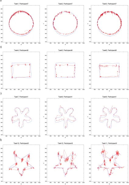
Fig 2shows eye and mouse trajectories for selected participants for all 12 tasks, one participant per form (each row). That is, in each row ofFig 2, we see the gaze and mouse trajectories of the same participant as they were tracing the respective geometric shape with our three tasks (‘nat-ural tracing’, ‘eyes-first’ and ‘mouse-first’). Note how the fixations are clearly observable on the gaze trajectory (the areas with a high concentration of gaze points). There are also noticeable tremors and drift within each fixation and while there are differences in how these look like between participants (e.g. tiny tremors/drifts for participant 1 inFig 2Cand large tremors/ drifts for participant 2 inFig 2D), the spatial pattern of these mini tremors and drifts is consis-tent for each participant across all three tasks (that is, across the entire row). Note also the dif-ference in geometric properties of the gaze and mouse trajectories for all participants and tasks: the jumpiness of eye-trajectories and the smooth continuity of the mouse trajectories.
Fig 2. Eye and mouse trajectories for selected participants for all twelve tasks: Natural tracing, eye-first, mouse-first for each geometric shape. Shapes: a) circle b) rectangle, c) curve and d) star. Eye trajectories are shown in red and
mouse trajectories in blue.
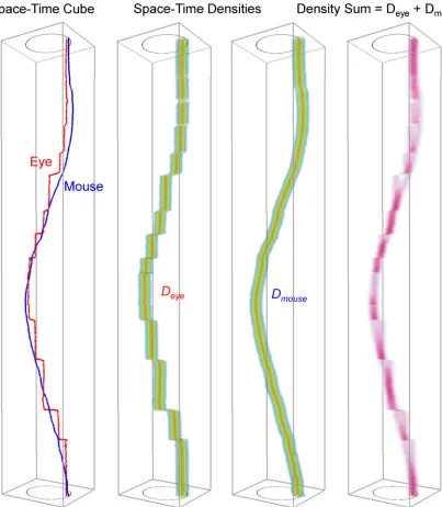
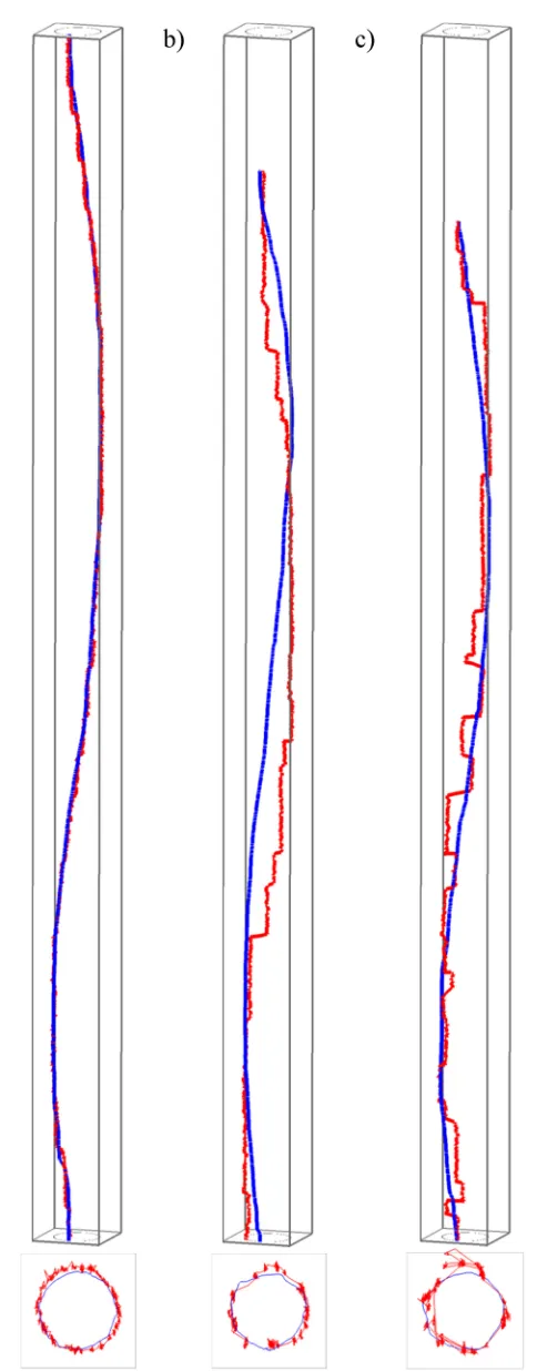
levels can be visualised.Fig 3shows one participant’s trajectories in the STCs, which are dis-played at the same spatial and temporal scale for the three tasks shown in this figure. Here, clear differences can be seen between the three tasks–observe how closely the eyes follow the mouse in natural tracing (task 1,Fig 3A), as the two trajectories in the STC differ only very slightly. The ‘eyes-first’ tracing (task 2,Fig 3B) produces the largest differences between the two trajectories and ‘mouse-first’ tracing (task 3,Fig 3C) somewhat smaller differences. Of note are two further observations; that these differences are almost indistinguishable when plotting trajectories only in 2D (see 2D projections at the bottom of the respective STCs inFig 3), and that surprisingly, already this one example contradicts one of our hypotheses: i.e. that there should be the most interaction and the least difference in the mouse-first task (task 3), where we expected the ‘smooth pursuit’ eye movement to occur. Visual inspection of eye and mouse trajectories from other tasks and other participants confirms this initial observation and we speculate that perhaps it is not fully possible or at least very difficult to consciously per-form ‘smooth pursuit’ for an object on the screen (the mouse pointer) that is moved indirectly through the use of another object (the mouse) manipulated by the hand. It is beyond the scope of this paper to further explore this effect, but we note that it could constitute an interesting research question.
Upon inspecting the acquired trajectories, we excluded data from one of the participants from further analysis. This participant consistently had 5% or more of gaze points outside the stimulus area on the screen (the majority of these spurious points were allocated to the coordi-nates of the origin point, even though the points just before and just after the spurious point were in the same other area of the screen, far from the origin), thus pointing to a potential sys-temic problem in eye tracker’s detection of this person’s gaze. As one of the goals of this exper-iment was to produce a data set that could be reliably used to test our new analytical method for quantifying the level of interaction between the gaze and the mouse, we decided to exclude the problematic participant. Our final data set therefore consists of gaze and mouse trajectories of ten participants (four females and six males) on twelve tasks. Anonymised gaze and mouse trajectories for all tasks and participants are provided as Supplementary Information (S1 Data).
Methodology for dynamic interaction between gaze and mouse
movements
In order to develop and evaluate new measures for the level of interaction between gaze and mouse movements, we conducted four separate types of analysis. First we used a traditional HCI evaluation measure, the time spent on task, in order to investigate the level of difficulty. In the second step we investigated the time series of distances between eye and mouse move-ments. In the third step we proposea new dynamic interaction measure for gaze and mouse movement, linked to foveal and parafoveal vision. In the fourth step we compare the measures from steps one and three to see if there is a connection between task times and levels of foveal and parafoveal dynamic interaction.
Analysis Step 1: Time spent on task
Fig 3. Differences in eye-mouse behaviour across the three tasks. A) task 1, b) task 2, c) task 3. Gaze
most difficult (task type: eyes-first) would have the longest average task times and that we should see a significant main effect of the task type in ANOVA results. In addition, the shape type could also matter–the two primitive shapes (circle/rectangle) were supposed to be traced faster than the two curved shapes (flower/star), regardless of the task type.
Analysis Step 2: Time series analysis of gaze-mouse distances
In this step, we considered gaze and mouse trajectories as time series of locations and calculate the distance between the gaze and the mouse at each moment in time.Fig 4shows three such distance time series for one participant while executing the three circle-tracing tasks (the same participant and the same tasks as those inFig 3). We then investigated the temporal distribu-tion of these distances across participants and tasks with the hypothesis that those tasks that are more difficult should have more variation in the gaze-mouse distances and thus the distri-butions of distance values in each time series should be wider than in series generated in easier tasks.
Analysis Step 3: Volumetric quantification of dynamic interaction
between eye and mouse movements
This section describes our new analytical methodology for quantifying dynamic interaction between gaze and mouse trajectories. We represent movement volumetrically, using space-time densities [24] in order to create what we call a ‘field of influence’ in the STC (see next sec-tion for a descripsec-tion). Then we appropriate a common remote sensing change detecsec-tion method to quantify the extent of interaction in the STC, and define the new dynamic interac-tion measure as the proporinterac-tion of interacinterac-tion voxels in the volume. This methodology is gen-eral and could be used for any type of movement. However, because our aim is to work with gaze and mouse trajectories in this project, we link the geometric parameters of the STC vol-umes to the characteristics of human vision, in particular to foveal and parafoveal vision.
Field of influence: A space-time density volume around each trajectory. We define a
new measure for quantifying dynamic interactions between the gaze and mouse trajectories based on an overlay of their respective ‘fields of influence’ within the three-dimensional envi-ronment of an STC. As mentioned earlier, the physics of eye and mouse movements differ in their basic characteristics, which means that comparing similarity of their trajectories is non-trivial. Mathematically, the comparison should be based on the progression of the two func-tions (curves) through a 3D space. Each trajectory is a function of timetand translatestinto a location on the 2D screen. One function (mouse trajectory) is continuous and smooth (differ-entiable) at eacht, while the other function (gaze trajectory) is, while continuous, not necessar-ily differentiable at eacht, since the almost-instantaneous saccades create jump discontinuities in the trajectory. In addition, during each fixation when the eye position should be stationary, the gaze trajectory is jiggled from the exact location of the fixating target through a combina-tion of small irregular tremors and drifts. The STCs inFig 3illustrate these two different behaviours.
In computational movement analysis, trajectories are compared based on their physical movement parameters [22], which are often calculated through differentiation on time (e.g. deriving velocity, acceleration and other parameters through numeric differentiation of
and at the same temporal scale (note the larger differences between eye and mouse for tasks 2 and 3, which require conscious intervention to both hand and eye movement). The lower image in each subpanel is a view from above, that is, a projection of trajectories onto the 2D space of movement.
Fig 4. Time series plots of eye-mouse distance. The same participant (no.9) [as inFig 3] executing the three tasks: a) task 1, b) task 2, c) task 3. For comparison, plots are shown at the same temporal (x axis shows time) and spatial (y axis shows distance) scales.
location coordinates). The non-differentiability of gaze trajectories means that these parame-ters cannot be calculated during saccades, when the eye is in transition between two fixations and when saccadic suppression occurs. In addition, during a fixation, the irregularity of trem-ors and drifts could affect the calculation of instantaneous velocity and acceleration and pro-duce artificial outliers that would prevent any direct comparison with the smooth movement of the mouse.
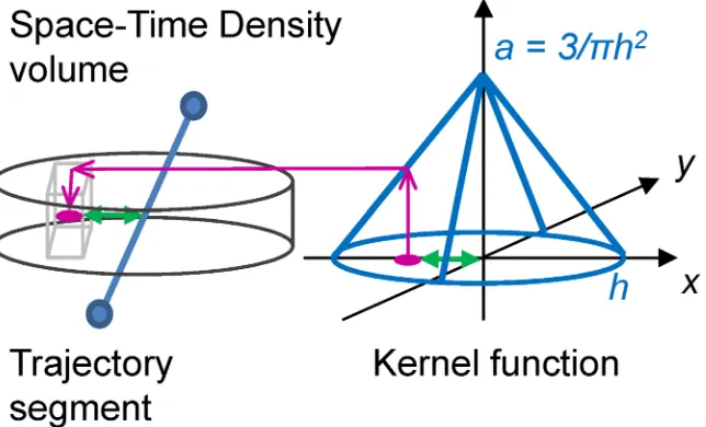
To address this, we propose to represent each movement as a volume, and compare the two volumes instead of directly comparing the shape of the two trajectories. Volumetric represen-tation of movement uses volumes, which are regular 3D grids consisting of voxels (unit cubes, analogous to pixels in a 2D grid). Movement is then represented through values of the proba-bility function calculated using a 2D spatial kernel at each voxel layer and centred on the movement trajectory. The resulting probability value is assigned to the respective voxel based on the distance of the voxel from the trajectory and the resulting volume is called the space-time density[24].
[image:16.612.204.526.411.606.2]In the context of gaze trajectories, this method of representing movement solves both prob-lems with saccadic jumps, and with irregular micro movements during fixations, as both these types of irregularities are smoothed with the application of the probability function. We there-fore calculate space-time densities for each separate trajectory of the gaze and the mouse. These density volumes consist of stacks of two-dimensional kernels, one kernel at each tempo-ral voxel layer (Fig 5). Each kernel is a 2D probability density function (PDF), centred on the gaze or mouse position at a particular moment in time. Similar PDFs have been recently used in eye-tracking to determine the probability of the user attending a certain object in a video game at a particular time [61]. In our case, as the layers of kernels are stacked one upon an-other through time, this builds a volumetric representation of movement which fills the entire
Fig 5. Building the space-time density volume from distance kernels around trajectory. At each voxel
layer, the algorithm finds the distance between each voxel (shown as a light-grey cube on the left) and the trajectory (in blue, distance shown with a green arrow), then assigns the value obtained from the kernel function at this particular distance in the kernel space (represented by the 3D coordinate system on the right) to the respective voxel. We link the kernel size (given by the radius h–the bandwidth) to the theory of foveal and parafoveal attention. We further assume that if a person is looking at a certain point, the attention away from the point will decrease linearly with distance and will be cut off at distance h, where h marks the boundary for foveal or parafoveal attention. We therefore use a linear kernel function in the form of a cone in kernel space.
STC. This density represents what we call a ‘field of influence’ around a trajectory and the task of comparing the two movement trajectories now becomes the task of comparing the two fields of influence. This is mathematically much simpler than comparing gaze and mouse tra-jectories directly, since the new comparison is between two volumes, and can be done voxel-wise.
We compare the two volumes using a change detection method generalised into the STC from remote sensing [25]. One of the most commonly used change detection methods in opti-cal remote sensing is image differencing [62]. In this method, two satellite images of the same area and of the same spatial resolution (pixel size) that are taken at two different times, are sub-tracted, pixel-by-pixel in order to build a difference image. The pixels of the difference image are classified into two groups, those that represent change, and those that represent no change, based on a pre-defined decision function which is set based on the characteristics of the phe-nomenon under observation. The result is a map of areas where change occurred between the two times when images were taken. We apply a similar principle to our two density volumes, generalising the image differencing idea into three dimensions and adapting the decision func-tion to the dynamic interacfunc-tion of gaze and mouse.
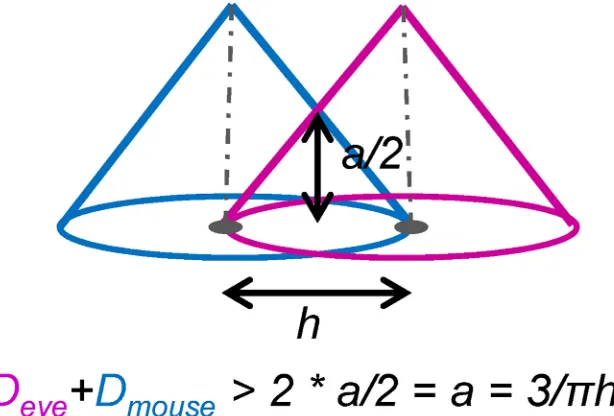
We calculate a voxel-by-voxel sum of gaze and mouse densities (Fig 6). The reason for choosing the sum as our algebraic operation rather than the original difference is that we are interested in areas in space and time when gaze and mouse are within each other’s field of influence.Fig 7illustrates this idea: imagine the position of the gaze as the centre of the pink kernel and the position of the mouse as the centre of the blue kernel. The width of the kernel, the bandwidth, is marked with h and the height of the kernel is equal toa = 3/πh2(see alsoFig 5) for the linear kernel to be a 2D PDF (which means that the volume under the kernel has to integrate to 1). We mathematically define the dynamic interaction to occur when the gaze and the mouse are closer to each other than the bandwidthh(we will further linkhto the concept of foveal/parafoveal attention). From this, we can calculate that for the dynamic interaction to occur, the two linear kernels need to intersect at the height ofa/2each, that is, the sum of the two kernels needs to be larger than2a/2
ora(Fig 7). This is the threshold to be used as a deci-sion function to classify voxels into interaction voxels vs. non-interaction voxels. In other words, if a voxel of the density sum volume has the value larger or equal toa, we count it as an interaction voxel.
The last step in the definition of the dynamic interaction measure is the normalisation of the count of interaction voxels with the total number of voxels in the volume. This is done in order to obtain a comparable measure of dynamic interaction for different cases and different volume sizes (note that volume sizes are dependent only on the time spent on task, since bases of all STCs are of the same size, i.e. the image stimuli from our experiment).
Method comparison. Our method is as far as we know the first method that attempts to
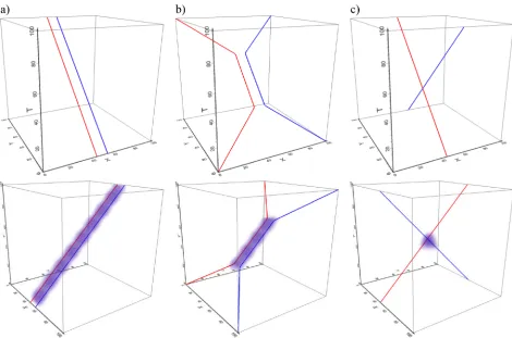
quantify the dynamic interaction between two physically diverse movement types. However, a number of methods exist for dynamic interaction between similar movement types, in particu-lar in movement ecology. To evaluate our method we therefore compare our dynamic interac-tion measure with two ecological measures [41] and as the latter two are not suitable for eye and mouse data, we do so on simulated trajectories. We created three cases with simulated data, each of which has a different levels of dynamic interaction (Fig 8). Simulated data are provided as Supplementary Information (S2 Data).
intersection of the home ranges of the two animals. Home range is a term from ecology, defined as the set of areas where an individual animal spends most of its time and there are a number of methods how this can be calculated from trajectory data [21]. For our three simu-lated cases we created the overlap zone for HAI as intersection of buffers around the two tra-jectories. We calculated the Prox and HAI values for all three simulated cases and compared them with our dynamic measure.
Sensitivity analysis. Our method uses the volumetric representation of movement and is
[image:18.612.156.559.75.537.2]therefore dependent on the resolution of the spatio-temporal partitioning of data space, that is the size of the voxels in the volume. Another parameter that can be adjusted is the kernel size,
Fig 6. Our proposed analytical methodology to quantify the level of interaction. From trajectories, through densities, to
density sum volume in which interaction voxels are counted.
which tells us how far from each trajectory does the field of influence reach. We investigated how the voxel size and the kernel size affect results by running two experiments on the same simulated data as above, where we kept one of the two parameters constant and changed the second parameter.
Linking interaction volume parameters to properties of human vision. The previous
section described the mathematical definition of our new measure for dynamic interaction and the process of its derivation. So far, the derivation was general and could be used for com-paring any two types of movement, however, as we are working with eye movement data we wanted to link it to the specifics of human vision. For this, we link the parameters of the space-time density to the concepts of foveal and parafoveal attention.
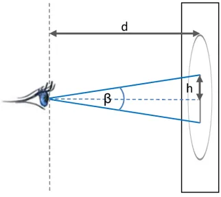
As described previously, the human visual field is spatially divided into three regions: foveal, parafoveal and peripheral, based on the angleβformed around the line of vision (Fig 9). Foveal region corresponds to the visual angle of 2˚, parafoveal region to the angle of 5˚ and the periphery corresponds to anything beyond the 5˚ [26,28]. We use the geometrical defini-tions of the foveal and parafoveal regions to set the values for the bandwidthhof our space-time densities. Given the distancedof the eyes from the screen and the size of the visual angle
β, we can calculate the radiushof the region that this particular visual angle covers:
h¼dtanðb=2Þ ð1Þ
[image:19.612.206.513.77.285.2]β/2is the angle between the visual axis, where the fovea is aligned to and the location away from the fovea and is also called the angle of eccentricity [30,27]. Given the parameters of our geometric setup we can calculate thehfor foveal and parafoveal regions and use these two val-ues to set the bandwidth for space-time densities for foveal/parafoveal interaction. This means that our dynamic interaction measure as defined above will identify the proportion of voxels where the mouse is closer to the eye thanh(as explained above and inFig 7), that is, within the foveal/parafoveal region respectively. This is similar to the 2D approach of Sundstedt et al. [63] who model the 2D energy spread of the gaze by placing a kernel on the location of the fixation
Fig 7. Definition of the dynamic interaction measure from the intersection of density volumes. We
define that dynamic interaction occurs in voxels where the two kernel centres are less than h apart from each other. In these voxels, values of the density sum are larger than twice the height at this distance from the centre, which is half of the total height of the linear kernel (a/2, see alsoFig 5).
(kernel is defined by the size of the foveal region) and use this kernel to link gaze to the geo-metric shape of the underlying object. In our case, the energy spread is modelled by the gaze kernel and the underlying object is the mouse, which is modelled through a separate kernel as explained above.Table 1provides values of geometric parameters calculated from the setup measures and used for derivation of the parameters for the two sets of space-time densities.
Differences in levels of foveal and parafoveal dynamic interaction. Once we obtained
the dynamic interaction measures for all participants in all tasks in this way, we investigated if there were any differences in the levels of foveal or parafoveal dynamic interaction for task types and geometric shapes. We ran two-way repeated measure ANOVAs to investigate the effect of the two factors or their statistical interaction on task time and the levels of foveal and parafoveal dynamic interactions. For this, we performed two two-way repeated measures ANOVAs with task type and geometric shape as the two factors, and respectively with foveal or parafoveal dynamic interaction as the dependent variable.
Analysis Step 4: Linking time spent on task to the level of dynamic
interaction
[image:20.612.104.574.74.385.2]In the final step of the analysis, we investigated if the time spent on task was related to the levels of foveal and parafoveal dynamic interaction. For this, we calculated correlation coefficients between time and both dynamic interaction levels respectively for each task.
Fig 8. Simulated data for method comparison with a) full dynamic interaction (case 1—trajectories parallel in space and time), b) middle
level dynamic interaction (case 2) and c) almost no dynamic interaction (case 3—trajectories parallel in space but not time). Bottom panels show our interaction volumes for each case (voxel size 2, kernel size 20).
Software and code
[image:21.612.204.526.75.362.2]The analysis was coded in Matlab and R and the 3D figures produced in Voxler software for volumetric visualisation. R code that implements our new analytical methodology (space-time densities and calculation of dynamic interaction between two trajectories) is provided as Sup-plementary Information (S1 Code). We used the R-package wildlifeDI for calculation of the two ecological indices Prox and HAI [41].
Fig 9. Linking density volume parameters to characteristics of human vision. Here, d is the fixed
distance from the participant to the screen (in our case 65cm), while h that we use as the kernel size for the density volume (seeFig 5), depends on the view angleβ(or rather, on one half of this angle,β/2).βis set to 2˚ for foveal interaction to 5˚ for parafoveal interaction.
https://doi.org/10.1371/journal.pone.0181818.g009
Table 1. Geometric parameters for calculation of gaze and mouse space-time densities.
Geometric parameter Value
Stimulus size 900 x 900 pixels
Pixel size* 0.265mm
Voxel size in x/y directions 10 pixels
Voxel size in t direction 10ms
Perpendicular distance d from eye to screen 65cm
Radius of foveal region (β= 2˚), calculated as per Eq (1) 1.135cm = 43 pixels Kernel size h for density foveal interaction calculation** 50 pixels
Radius of parafoveal region (β= 5˚), calculated as per Eq (1) 2.838cm = 107 pixels Kernel size h for density in parafoveal interaction calculation** 110 pixels
*Pixel size was calculated as the ratio between screen height (cm) and height of the stimulus image (pixels).
**Radius rounded to the first next multiple of voxel size in x/y directions.
[image:21.612.200.576.533.662.2]Results
Analysis Step 1: Time spent on task
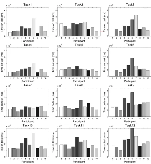
[image:22.612.83.573.168.699.2]Fig 10shows bar charts of times spent on task per task and participant, shown at the same scale. Mean times and standard deviations for each task are shown inTable 2.
Fig 10. Times spent on task. Times are shown on the same scale per task and participant.
Interestingly, we do not see the expected increase in task times for tasks with the eyes-first tracing method (the middle column ofFig 9). However, unsurprisingly, we see an increase in the time-use across geometric shapes, with the two simpler shapes (the rectangle and the circle) that are composed of shorter lines and fewer turns having the shortest completion times, fol-lowed by the curve and the star. In particular, the star stands out as the shape requiring the lon-gest times. Across tracing methods, there is more variation, but on the whole, it was the third type of tracing (mouse-first, the right column ofFig 9) that people used the longest time to perform.
The two-way repeated measures ANOVA on task time confirmed observations from the pre-vious paragraph. There is a significant main effect of task type (F = 4.1555, p = 0.0328<0.05), there is a highly significant main effect of geometric shape (F = 14.0760, p = 6.183710−6
<0.001) and there is a significant effect of statistical interaction between the two factors (F = 3.4133, p = 0.0063<0.05).Fig 11shows the ANOVA plot. Interestingly (and somewhat contradictory to our expectations), the longest mean times are for task type 3 (mouse-first), rather than task type 2 (eyes-first), which we hypothesised would be the most difficult task to execute.Fig 11also shows that the ANOVA interaction is between these two task types, while the task type 1 (natu-ral tracing, shown with a green line inFig 11) is separate with the shortest mean times for all four geometric shapes.
Analysis Step 2. Time series analysis of eye-mouse distance
Fig 12shows the box-and-whiskers plots of variations of eye-mouse distances. That is, for each eye-mouse distance time series we take all distance values and produce one plot per task and participant. All plots are shown at the same scale and all participants in the same order, to make subpanels of this Fig visually comparable with each other. Each box is crossed by the red median line and defined by the 25thand 75thpercentiles. The whiskers extend to 1.5 intra-quartile differences on each side and all points beyond that are individually plotted as outliers (in red).
[image:23.612.40.577.108.285.2]The distribution of distance values in each time series can be investigated looking at the sizes of the boxes and the length of the whiskers. In general, natural tracing tasks (the left col-umn ofFig 12) have the smallest boxes, the eye-first tasks (the central column ofFig 12) have
Table 2. Mean and standard deviation of times spent on task. Note that the task numbering here (1–12) is for convenience of reporting, and it does not
express the task types as introduced in the experiment design section. To make the link, the ‘tracing method’ column is important (i.e., experimental tasks are repeated based on tracing method per shape type).
Task No. Shape (Task type #) Tracing method Time on task (ms):
Mean St Dev
1 Circle (1) Natural 11583 6908.4
2 Circle (2) Eyes-first 15868 4713.0
3 Circle (3) Mouse-first 14902 8165.3
4 Rectangle (1) Natural 10385 4543.1
5 Rectangle (2) Eyes-first 11310 2242.6
6 Rectangle (3) Mouse-first 12788 6475.5
7 Curve (1) Natural 12888 2945.1
8 Curve (2) Eyes-first 15675 4412.1
9 Curve (3) Mouse-first 20926 7810.8
10 Star (1) Natural 18808 8228.3
11 Star (2) Eyes-first 19290 5956.2
12 Star (3) Mouse-first 23606 9815.1
the largest boxes with only a few outliers, while the mouse-first tasks show more individual variation (e.g. participant no. 9 has consistently a much larger box in the mouse-first tasks than any other participant, see the third column ofFig 12). This seems to indicate that when naturally tracing a shape, the gaze and mouse are consistently closer at each moment in time than when tracing with eyes-first–a result that confirms our hypothesis that there should be the least interaction between gaze and mouse in eyes-first tasks. The results for mouse-first are less clear (the right column ofFig 12)–while boxes in the respective plots are similarly narrow as in natural tracing tasks, there are substantially larger outliers present for several individuals, including one individual (no. 9) whose distribution of distance values for mouse-first tasks is similar to his/her pattern for eyes-first task rather than natural tracing tasks.
Analysis Step 3: Quantifying the dynamic interaction
Method comparison. The Prox and HAI indices show the expected pattern in the
[image:24.612.100.574.72.472.2]interac-tion level for our three cases: case 1 –high interacinterac-tion, case 2 –mid-level interacinterac-tion and case
Fig 11. ANOVA plot for time spent on task. The plot shows ANOVA interaction between task type and geometric shape. Task types are:
1 –natural tracing, 2 –eyes-first and 3 –mouse-first. Shapes are: 1 –circle, 2 –rectangle, 3 –flower and 4 –star.
3—low interaction. Our measure (DI Eye-Mouse) shows the same decreasing pattern (Table 3). Note that Prox and HAI values are the same for cases 1 and 3, due to the definition of the overlap zone, which for these simulated data means that in both cases all trajectory fixes
Fig 12. Box-and-whiskers plots of gaze-mouse distance per participant. Plots are shown for tracing a) the circle, b) the
rectangle, c) the curve and d) the star. Each row shows three charts: for natural tracing, for eye-first and for mouse-first. Each boxplot in each chart is the distribution of eye-mouse distance for one participant, where participants are ordered in the same way across all charts and all charts are shown at the same scale, to allow for visual comparison across each geometric form (per row) and across all forms (per column).
are counted for both indices. Note also that while Prox and HAI have a fixed range from [0,1], this range depends on the concept of home range, which is a spatial concept and does not take into consideration time. Our measure in contrast normalises the interaction using the spatio-temporal volume, meaning that the values are significantly lower in comparison with the eco-logical indices because of the inclusion of time into the normalisation.
Sensitivity analysis. Table 4shows the results of both experiments, where in the first one we kept the kernel size constant and varied voxel size and in the second one did the opposite.
Fig 13shows these values broken down by voxel/kernel size in each respective experiment. The pattern where interaction decreases from case 1 to case 3 is the same in all cases, regardless of voxel or kernel variation. Further, the values of the measure increase with kernel size and decrease with voxel size, both of which are expected patterns. These are typical behaviours of algorithms on discretised space representations, such as for example raster algorithms—in our case, we have generalised them into the volumetric space.
Quantifying foveal/parafoveal interaction. To analyse the level of dynamic interaction
[image:26.612.200.578.89.140.2]between the gaze and the mouse within foveal/parafoveal regions, we plotted our dynamic interaction ratios as bar charts per task and per participant (Figs14and15). Participants are ordered in the same way in all plots in these two Figs and each participant is represented with a consistent shade of grey of respective bars in order to allow for visual comparison of the same person’s performance in all tasks and at both foveal and parafoveal levels. All plots are also scaled the same for foveal interaction and for parafoveal interaction respectively, allowing visual comparison of subpanels within each figure.
Table 3. Values of dynamic interaction indices for three simulated data cases.
Case Prox HAI DI Eye-Mouse
1 1 1 0.02371
2 0.445545 0.714286 0.01079
3 0.168317 0.168317 0.00355
[image:26.612.41.576.479.704.2]https://doi.org/10.1371/journal.pone.0181818.t003
Table 4. Values of our dynamic interaction measure vs. voxel size and vs. kernel size. In the first two columns we varied the voxel size while keeping
the kernel size constant (20). The last two columns show results where kernel size was varied at a constant voxel size (2).
Experiment 1 Experiment 2
Constant kernel size = 20 Constant voxel size = 2
Case Voxel size DI Eye-Mouse Kernel size DI Eye-Mouse
1 0.5 0.0258 20 0.02371
1 1 0.02508 40 0.1044
1 2 0.02371 60 0.23121
1 5 0.01976 80 0.39322
1 10 0.01277 100 0.58573
2 0.5 0.01161 20 0.0108
2 1 0.01123 40 0.06016
2 2 0.0108 60 0.16824
2 5 0.00864 80 0.32589
2 10 0.00676 100 0.52475
3 0.5 0.00365 20 0.00355
3 1 0.00356 40 0.03469
3 2 0.00355 60 0.12107
3 5 0.00281 80 0.2911
3 10 0.0015 100 0.57259
The ANOVA of foveal dynamic interaction showed a highly significant main effect of task type (F = 36.3164, p = 4.807110−7
<0.001), a significant main effect of shape type (F = 3.6593, p = 0.0247<0.05) and no significant effect of statistical interaction (F = 1.8896, p = 0.0994>
0.05). The ANOVA on parafoveal dynamic interaction showed a highly significant main effect of task type (F = 53.6080, p = 2.621310−8<0.001), a significant main effect of shape type (F = 5.5663, p = 0.0042<0.05) and no significant effect of statistical interaction (F = 1.8122, p = 0.1140>0.05).Fig 16shows ANOVA plots for foveal and parafoveal dynamic interaction respectively. In both plots, the lowest mean dynamic interaction is in task type 2 (eyes-first), which confirms our expectation that as this would be the most difficult task to perform (i.e., this is the task where we expected to see the lowest level of dynamic interaction between the gaze and the mouse). Surprisingly however, in both cases, the highest mean dynamic interac-tion occurs in task type 1 (natural tracing) rather than in task type 3 (mouse-first), which con-tradicts our expectation that there would be the smooth pursuit type of eye movement in task type 3 and consequently the highest level of dynamic interaction.
Analysis Step 4. Linking time and interaction
[image:27.612.141.573.74.283.2]Table 5shows correlation coefficients between time spent on task and the levels of foveal and parafoveal dynamic interaction respectively. We calculated these two values per task and found that for task type 1 (natural tracing tasks, i.e., task numbers 1, 4, 7 and 10), task times seem to be relatively highly correlated with the dynamic interaction levels. This is however not so for the other two task types (eyes-first, mouse-first); perhaps suggesting that there is a natu-ralcoupling between the eye and the mouse movements during route tracing, but this coupling breaks when a participant tries to use the gaze or the mouse intentionally (consciously) in a particular way. Since both eyes-first and mouse-first task types require the participants to use the parafoveal (or even peripheral) vision to some degree, we might be documenting an instance of covert attention. This is an interesting finding, and upon further testing to confirm, it is imaginable that it could serve as an additional metric in eye tracking studies to understand whether the participants might be working with covert attention.
Fig 13. Sensitivity to method parameters shown on simulated data. Panel a) shows changes in method results for varying
voxel sizes while kernel size is kept constant. Panel b) varies kernel size for a constant voxel size. The pattern of interaction value decreasing from case 1 through 2 to 3 is the same, regardless of voxel or kernel size.
Conclusions and discussion
[image:28.612.95.579.94.588.2]In this paper we introduce a new analytical methodology for quantifying dynamic interaction between gaze and mouse movements in a route tracing experiment. The methodology is based
Fig 14. Quantifying foveal interaction. Plots are shown for tracing the circle (tasks 1–3), the rectangle (tasks 4–6), the curve (tasks 7–9)
and the star (tasks 10–12). Each row shows three charts: for natural tracing, for eye-first and for mouse-first. Participants are ordered in the same way across all charts and all charts are shown at the same scale, to allow for visual comparison of charts across each geometric form (per row) and across each participant (per each bar in each chart). Bars are coloured per participant in this and the next figure (parafoveal interaction).
on recent developments in computational movement analysis and visualisation within
[image:29.612.92.577.94.569.2]GIScience and Remote Sensing. We further make use of experiment designs based on the prin-ciples of experimental psychology and HCI. This paper is therefore one of the first attempts at interdisciplinary knowledge exchange between these disciplines (computational movement analysis, GIScience, Remote Sensing psychology, vision science and HCI).
Fig 15. Quantifying parafoveal interaction. Plots are shown for tracing the circle (tasks 1–3), the rectangle (tasks 4–6), the curve (tasks
7–9) and the star (tasks 10–12). Each row shows three charts: for natural tracing, for eye-first and for mouse-first. Participants are ordered in the same way across all charts and all charts are shown at the same scale, to allow for visual comparison of charts across each geometric form (per row) and across each participant (per each bar in each chart). Bars are coloured per participant in this and the previous figure (foveal interaction).
Our first aim was the introduction of the novel analytical methodology for comparison of dynamic interaction of gaze and mouse trajectories. We successfully demonstrated how bespoke spatio-temporal methods can solve the problem of comparing two movement types that are very different in terms of physics, and how the proposed method allows processing the data that these two movement processes generate.
We further tested our method against established methods for dynamic interaction in movement ecology. Ecological indices measure interaction between two physically similar movement types as well as depend on specific ecological concepts, such as home range [41] and are therefore not suitable for gaze and mouse data. For this reason we did not evaluate our method against them on real eye and mouse data, but created data for three simulated scenar-ios with different levels of interaction. This pattern was identified with all methods.
[image:30.612.125.577.77.285.2]We also performed a sensitivity analysis to the two method parameters (voxel and kernel size). We found that our measure is sensitive to both, but that it increases/decreases consistently
Fig 16. ANOVA plots for the foveal and parafoveal dynamic interaction measures.
https://doi.org/10.1371/journal.pone.0181818.g016
Table 5. Correlation coefficients between time on task and the two types of dynamic interaction. Note that natural tracing tasks have high correlations
between task times and foveal/parafoveal interactions (shown on grey fields).
Task No. Shape (Task type #) Tracing method Correlation between time on task and:
foveal interaction parafoveal interaction
1 Circle (1) Natural 0.65003 0.63267
2 Circle (2) Eyes-first 0.34971 0.27819
3 Circle (3) Mouse-first 0.055692 -0.1871
4 Rectangle (1) Natural 0.81515 0.77223
5 Rectangle (2) Eyes-first -0.47987 -0.1705
6 Rectangle (3) Mouse-first -0.22204 -0.28724
7 Curve (1) Natural 0.76818 0.72107
8 Curve (2) Eyes-first -0.36521 -0.44811
9 Curve (3) Mouse-first -0.37321 -0.28992
10 Star (1) Natural 0.81328 0.7165
11 Star (2) Eyes-first -0.24797 0.071006
12 Star (3) Mouse-first 0.053052 0.11458
[image:30.612.38.577.529.705.2]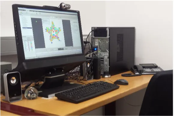
![Fig 4. Time series plots of eye-mouse distance. The same participant (no.9) [as in Fig 3] executing thethree tasks: a) task 1, b) task 2, c) task 3](https://thumb-us.123doks.com/thumbv2/123dok_us/8997678.396575/15.612.196.470.73.685/series-plots-mouse-distance-participant-executing-thethree-tasks.webp)