Derivatives Pricing via Machine Learning

(1)

ISSN Online: 2162-2442 ISSN Print: 2162-2434

DOI: 10.4236/jmf.2019.93029 Aug. 27, 2019 561 Journal of Mathematical Finance

Derivatives Pricing via Machine Learning

Tingting Ye

1

_{, Liangliang Zhang}

2

1_{Department of Accounting, Questrom School of Business, Boston University, Boston, MA, USA} 2_{Bank of America, Charlotte, NC, USA}

Abstract

In this paper, we combine the theory of stochastic process and techniques of machine learning with the regression analysis, first proposed by [1] to solve for American option prices, and apply the new methodologies on financial derivatives pricing. Rigorous convergence proofs are provided for some of the methods we propose. Numerical examples show good applicability of the al-gorithms. More applications in finance are discussed in the Appendices.

Keywords

Machine Learning, Regression Analysis, Jump-Diffusion, Derivatives Pricing, Hilbert Space, Orthogonal Projection

1. Introduction

Theoretical and empirical finance research involves the evaluation of conditional expectations, which, in a continuous time jump-diffusion setting, can be related to second order partial integral differential equations of parabolic type (PIDEs) by the Feynman-Kac theorem, and other types of equations such as backward stochastic differential equations with jumps (BSDEJs) or quasi-linear PIDEs in more complicated settings. In theoretical continuous-time finance, many prob-lems, such as asset pricing with market frictions, dynamic hedging or dynamic portfolio-consumption choice problems, can be related to Hamil-ton-Jacobi-Bellman (HJB) equations via dynamic programming techniques. The HJB equations, from another perspective, are equivalent to BSDEs derived from a probabilistic approach. The nonlinear BSDEs, studied in [2], can be decom-posed into a sequence of linear equations, which can be solved by taking condi-tional expectations, via Picard iteration. For empirical studies, the focus of the literature has been the evaluation of the cross sectional conditional risk-adjusted expected returns and the explanation of them using factors. See [3][4] and [5] as

How to cite this paper: Ye, T.T. and Zhang, L.L. (2019) Derivatives Pricing via Machine Learning. Journal of Mathematical Finance, 9, 561-589.

https://doi.org/10.4236/jmf.2019.93029 Received: May 22, 2019

Accepted: August 24, 2019 Published: August 27, 2019 Copyright © 2019 by author(s) and Scientific Research Publishing Inc. This work is licensed under the Creative Commons Attribution International License (CC BY 4.0).

(2)

DOI: 10.4236/jmf.2019.93029 562 Journal of Mathematical Finance

good illustrations. It is easily seen that, regardless of the fact whether the under-lying models are continuous-time or discrete-time, evaluating conditional ex-pectations is inevitable in finance literature. Moreover, in order to perform XVA computations for the measurement of counterparty credit risk, we need to eva-luate the conditional expectations, i.e., the derivative prices, on a future simula-tion grid, as outlined in [6]. These facts call for efficient methods to compute the quantities aforementioned.

In this paper, we extend the basis function expansion approach proposed in [1]

with machine learning techniques. Specifically, we propose new efficient me-thods to evaluate conditional expectations, regardless of the dynamics of the underlying stochastic process, as long as they can be simulated. Rigorous con-vergence proofs are given using Hilbert space theory. The methodologies can be applied to time zero pricing as well as pricing on a future simulation grid, with the advantage of ANN approximation most prominent in high dimensional problems. In the sequel, we show applications of our methodologies on the pricing of European derivatives and extension to contracts with optimal

stop-ping feature is straightforward through either [1] approach or

reflect-ed-BSDEs.

Compared to the literature on traditional stochastic analysis, our methodolo-gies are able to handle large data sets and high-dimensional problems, therefore suffering much less from the curse of dimensionality due to the nature of ANN methods. Moreover, our methodologies are very efficient when evaluating solu-tions of BSDEJs and PIDEs on a future simulation grid, where none of the tradi-tional methodologies applies. With respect to recent machine learning literature on numerical solutions to BSDEs and PDEs, our methodologies enjoy the theo-retical advantage of being able to handle equations with jump-diffusion and convergence results are provided. When applied to the solutions of BSDEJs and PIDEs, our methodologies require much less number of parameters, as com-pared to the current machine learning based methods to be mentioned below. At any step in the solution process, only one ANN is needed and we do not require nested optimization. In terms of application, not all the prices of OTC deriva-tives can be easily translated into BSDEJs and PIDEs, for example, a range ac-crual with both American and barrier (knock-out, for example) feature. Howev-er, our methodologies are naturally suitable in those situations. To conclude, our methods enjoy many theoretical and empirical advantages, which makes them attractive and novel.

There has been a huge literature on applications of machine learning tech-niques to financial research. Classical applications focus on the prediction of market variables such as equity indexes or FX rates and the detection of market anomalies, for example, [7] and [8]. Option pricing via a brute-force curving

fit-ting by ANNs dates back to [9]. More applications of machine learning in

(3)

our methods compared to this reference. First of all, we enable deep neural net-work (DNN) approximation and show convergence. Second, we can incorporate constraints in DNN approximation estimation and prove the mathematical va-lidity of this approach. Third, we propose two more efficient methods to com-plement the first method of ours. Our treatment of constraints in the estimation of DNNs extends the work of [12] in that we can deal with a larger class of con-straints by specifying a general Hilbert subspace as the constrained set. Risk measure computation using machine learning can be found in [13]. Applications of machine learning function approximation on financial econometrics can be found in [14], [15], [16] and [17]. Recent applications include empirical and theoretical asset pricing, reinforcement learning and Q-learning in solving dy-namic programming problems such as optimal investment-consumption choice, option pricing and optimal trading strategies construction, e.g., [18], [19], [20],

[21], [22], [23], [24], [25], [26], [27], [28] and references therein. Numerical methods to solve PDEs and BSDEs or the related inverse problems can be found in [29], [30], [31], [32], [33], [34], [35], [36], [37], [38] and [39]. Machine learning based methods enjoy the advantage of being fast, able to handle large data sets and high dimensional problems.

Our methodologies are combinations of traditional statistical learning theory and stochastic analysis with advanced machine learning techniques, introduc-ing powerful function approximation method via the universal approximation theorem and artificial neural networks (ANNs), while preserving the regres-sion-type analysis documented in [1]. The methods are very easy to use, effec-tive, accurate as illustrated by numerical experiments and time efficient. They are different from the convergent expansion method, e.g., [40], simulation methods such as [41], [42], [43] and [44] or the asymptotic expansion method proposed by [45], [46], [47], [48] [49] [50] [51] [52], in that we no longer resort to polynomial basis function expansion or small-diffusion type analysis. Our methods are also different from the pure machine learning based ones documented in [29], [30], [31], [32], [33], [34] and [35], in that we utilize the lead-lag regression formula to evaluate the conditional expectations, preserv-ing the time dependent structure and our methods are able to handle jump-diffusion processes easily.

The organization of this paper is as follows. Section 2 documents the metho-dologies. Section 3 illustrates the usefulness of our methods by considering Eu-ropean and American derivatives pricing. Section 4 considers numerical experi-ments and Section 5 concludes. An outline of the proofs and other applications can be found in the appendices.

2. The Methodology

Mathematical Setup

(4)

(

)

(

)

(

)

(

)

0 0

dXt =

µ

t X, t dt+

σ

t X, t dWt+

∫

_E

γ

t X e N t e, ,t  d ,d , X =x (1)

where

_X

_∈

_

r_, _W_∈_d_{is a standard}_d_{-dimensional Brownian motion and}

N is a q-dimensional compensated Poisson random measure, with the

com-pensator ν

(

d ,d :t e

)

=ν

( )

d de t_{. Information filtration} W N,

t = t

  is generated

by

(

W N,

)

. We hope to evaluate the conditional expectation t

ψ

( )

XT  for

any 0< <t T_{, e.g., see}_[53]_{. Assumptions on}ψ_and_X_{are stated below.}

Assumption 1 (On Growth Condition of ψ). ψ _{has polynomial growth in}

its argument x, i.e., there exists a positive integer P, independent of x, such that for all x >1_,_{we have}_,_{for constant C independent of x}

( )

x C xP.

ψ ≤ (2)

The following assumption is w.r.t. X.

Assumption 2 (On X). There exists a unique strong solution to Equation (1)

and X has finite polynomial moments of all orders.

The General Approximation Theory

First, we need the following assumptions, definitions and results. Please note that, some of the spaces we introduce are actually conditional ones. The discus-sions of conditional Hilbert spaces can be found in [54], e.g., 2

( )

t

L  is a

con-ditional Hilbert space for all t∈

[ ]

0,T _.

Definition 3 (Projection Operator). For Hilbert spaces  and , where

⊂

  . Define PROJx as the projection of x∈ onto .

Definition 4 (Orthogonal Space). For Hilbert spaces  and , where

⊂

  . Define ORTH as the orthogonal space of  in .

Definition 5 (Spanning the Hilbert Space). Assume that

{ }

j

j e _∈Λ

=

 is a

set of elements in Hilbert space  and Λ_{is an index set. Define}H as the

intersection of all Hilbert subspaces of  containing  .

Assumption 6 (On Joint Continuity).  and  are two Hilbert spaces

and _⊂__{. Moreover}_,

{ }

_{n n}∞₌₁ is a sequence of Hilbert sub-spaces of  sa-tisfying n⊂n+1 for any n≥1 and n₁ n

∞

= =



  . We have

limn→∞ h−PROJ_nhn _=0 for any h∈ and limn→∞hn=h.

The next two theorems are well-known in the literature.

Theorem 7 (Hilbert Projection Theorem). Let _⊂_ _{be two Hilbert}

spaces and let x∈. Then, PROJx exists and is unique. Moreover, it is

characterized uniquely by x−PROJ_x∈ORTH_ .

Theorem 8 (Repeated Projection Theorem). Let ⊂⊂ be three

Hilbert spaces. Then, for any x∈, PROJ_x=PROJ PROJ_

(

_x

)

_.

Remark 9 The conditions of Theorems 7 and 8 on  and  can be re-laxed to convexity and completeness instead of Hilbert sub-spaces.

Finally, we have the result below.

Theorem 10. Suppose  is a Hilbert space,

{ }

n n1

∞ =

 and  are Hilbert

subspaces of  satisfying n⊂n+1 and n1 n

∞

= = ⊂

(5)

PROJ _n

n

h = _ x_and h=PROJ_x_{. Then we have} limn→∞hn=h w.r.t. the norm

topology in , if Assumption 6 is satisfied.

Sometimes we need to add constraints on the calibrated ANN, e.g., the shape constraints. The following assumption and theorem deal with this situation.

Assumption 11 (On Constrained Sub-space). Suppose that Ψ ⊂ such

that

{

_{n n}

}

∞₁ =

Ψ is a sequence of non-empty convex and complete subspaces of  satisfying Assumption 6, where  and

{ }

_{n n}∞₁

=

 are described.

The following theorem handles the constrained approximation and its con-vergence.

Theorem 12 (On Constrained Approximation). Under Assumptions 6 and

11, for x∈, if h=PROJ_x∈ Ψ_,_then_,_{we have} limn→∞PROJΨ_nx h= . Remark 13 (On ψ). In Theorem 12, the set Ψ represents prior knowledge on constraints that h satisfies. It can be represented by a set of non-linear in-equalities or in-equalities on functionals of h. Common constraints for option pricing include non-negativity constraint and the positiveness constraint on the second order derivatives. The verification of

{

_{n n}

}

∞₁

=

Ψ satisfying Assump-tion 6 should be based on a case-by-case manner.

To proceed further, we need the following assumptions.

Assumption 14 (On Some Spaces).

{ }

J ₁

t _J

∞ =

 is an increasing sequence of

Hilbert sub-spaces of 2

( )

t

L  , J J 1

t ⊂ t +

  , 2

( )

1

J

t t t

J L

∞

= = ⊂



   . Moreover,

[ ]

( )

[ ]

( )

{

_| 2 _, 2

}

2

( )

2

( )

t ξT ξT∈L T t ξT ∈L t ⊂ t⊂L t ⊂L T = T

        .

Assumption 15 (On Structure of J

t

 ).

{ }

j t _j

e _∈Λ is a set of elements of

( )

2

t

L  , such that H

_{{ }}

j t j J

J

t _e

∈Λ

=

 , where Λ ⊂ ΛJ J+1⊂ Λ for any J≥1 and

1 J J ∞

=Λ = Λ



, satisfies Assumption 141_.

Then, we have the following results.

Lemma 1. For any adapted stochastic process

ξ

such that 2

( )

T L T

ξ

∈  , if

[ ]

2

( )

t

ξ

T ∈L t

  , we have

[ ]

( )

(

)

2

arg min .

t t

t T T t

L

η

ξ ξ η

∈

 

= _ − _

 

 (3)

The following proposition is a natural extension of Lemma 1.

Proposition 16. For any measurable function ψ _{and stochastic process X}

such that

( )

2

( )

T T

X L

ψ

∈  and

( )

2

( )

t

ψ

XT ∈L t

  , we have

( )

(

( )

)

2

arg min .

t t

t T T t

L

X X

ξ

ψ ψ ξ

∈   = −     _ _  

 (4)

Here ξ ∈t t and the above minimization problem has a unique solution. In

particular, if X is a Markov process, then ξt =φ

(

t X, t

)

, i.e., ξt is a function of

time t and Xt.

We then have the following theorem.

1_{It is obvious that}

{ }

j

t j

e ∈Λ can be the basis or frame of

( )

2

t

(6)

Theorem 17. Under Assumptions 1, 2, 6, 14 and 15, for any adapted stochas-tic process

ξ

such that 2

( )

T L T

ξ

∈  and

[ ]

2

( )

t

ξ

T ∈L t

  , we have

(

)

2_{( )}

[ ]

2

lim arg min_J .

t

t t T t L t T

J→∞ η∈

ξ η

ξ

 ₋ ₌

 

 _ 

 (5)

Further, for any measurable function ψ and stochastic process X such that

( )

2

( )

T T

X L

ψ

∈ _ _and

( )

2

( )

t

ψ

XT ∈L t

  , we have the following equality

( )

(

)

2_{( )}

( )

2

lim arg min_J .

t

t t T t L t T

J→∞ ξ∈ ψ X ξ ψ X

 ₋ ₌ __ __

 

 

 _ 

 (6)

If X is Markov, then we have ξt =φ

(

t X, t

)

, i.e., ξt is a function of time t and t

X .

The following theorem justifies the Monte Carlo approximation of expecta-tion in the above optimizaexpecta-tion problems.

Theorem 18 (On Sequential Convergence). Under Assumptions 1, 2, 6, 14

and 15, suppose that Λ =J mJ < ∞ for all J≥1,

{ }

₁ M i T i

X ₌ and

{ }

, , , 1,1

J

m M j i t _{j i}

e ₌

are M i.i.d. copies of XT and

{ }

₁

J

m j t _j

e ₌ . Then we have

( )

(

)

2

( )

=1

1

lim lim arg min_m _J .

t t

M

m m

T t t T

J→∞M→∞ ξ ∈ M _m

∑

ψ

X −

ξ

=  

ψ

X  (7)

The following results justify the universal approximation and ANN approxi-mation approaches proposed in this paper.

Proposition 19 (On Universal Approximation Theory). Let

σ

denote the

function in the universal approximation theorem mentioned in [55], [56] and [57]. Define

{ }

_j mn₁:

{

(

)

}

mn₁

t _j j j t _j

e

σ α

β

X

= = + = , where X satisfies Equation (1) and

Assumption 2, αj and βj have at most n significant digits in total, where n∈__,_i.e._,_{n belongs to the set of natural numbers}_,_{j runs from}₁_to m_n and

n

m is the number of all related

{ }

j t

e , i.e.,

(

)

{

| and have at most total significant digits

}

n t

m = σ α β+ X α β n . Then,

{ }

₁

H jmn t j e n = _∈           

satisfies Assumptions 6, 14 and 15. Therefore, Theorems 17 and

18 apply.

Proposition 20 (On Deep Neural Network Approximation). For the DNN

defined in ([58], Definition 1.1], observe that W xl

( )

=αl+βlx. Define

( )

, 1, 1,

:

j

t L j L j j t

e =W _{ }

ρ

W ₋ _{ }

ρ

W _

ρ

X ₍₈₎

where Wl j,

( )

x =αl j, +βl j, x satisfies that

l

=

1,2, ,



L

,

(

α β

l j, , l j,

)

have at most n total significant digits and n∈. Then,

_{{ }}

1

1,

H jmn t j e n = _∈           

, where 1 means

function f x

( )

≡1_{for all x}_,_{satisfies Assumptions}_{6, 14}_and_15._Therefore_,

Theorems 17 and 18 apply after a localization argument on ψ _{and X on a} compact sub-domain in

_

r_.

(7)

show convergence when the number of connections goes to infinity, which can be achieved via enlarging the number of neurons in each layer with the total number of layers remaining fixed.

Remark 22 (On Euler Time Discretization). [59]proposes an exact

simula-tion method for multi-dimensional stochastic differential equasimula-tions. The discus-sion of discretization error, of the regression approach proposed in this paper,

with Euler method is not hard if ψ_{satisfies Assumption}1, in which case the dominated convergence theorem and

_L

2_{convergence of Euler method can be} applied to show the convergence.

The proofs of the above results can be found in Appendix A. In what follows, we will propose three methods to compute, approximately, the function

φ

in Proposition 16.

Method 1

In general,

φ

, defined in Proposition 16 and Theorem 17, can not be found in closed-form. A natural thought would be to resort to function expansion repre-sentations, i.e., to find the solution to the following problem

( )

{ } ₀

( )

(

)

2

, 0

arg min , |

j _{j j}

j

t T T j t j

a j

X X a e t X

θ

ψ _∞ ψ θ

= ∞ ∈ = _ _    = −       _ _   

∑

  

 (9)

where  is an appropriate space for coefficients

{

aj,θ_{j j}

}

₀ ∞

= and

{

( )

}

0

j

j _j

e

θ

∞

=

is a set of functions, with Span

(

{

j

( )

}

₀

)

j _j

e θ ∞

=

2_{dense in an appropriate function}

space Φ3_{. To further proceed, we seek a truncation of the function}

representa-tion formula as follows

( )

{ } ₀

( )

(

)

2

, 0

arg min_J , |

j j _j J

J j

t T T j t j

a j

X X a e t X

θ

ψ ψ θ

=∈ = _ _    ≅ −   _ _   _ _   

∑

  

 (10)

for J sufficiently large, where J is a compact set in the Euclidean space where

{

a_j,θ_{j j}

}

J ₀

= take values. The last step would be to use Monte Carlo simulation to

approximate the unconditional expectation appearing in Equations (9) and (10). Therefore turning the conditional expectation computation problem, into a least-square function regression problem, similar to [1]. An obvious choice of

( )

{

j

}

₀

j _j

e

θ

∞

= is polynomial basis, for example, the set of Fourier-Hermite basis

functions. For expansion using Fourier-Hermite basis functions in high dimen-sions, see [60].

In fact, Artificial Neural Networks (ANNs) prove to be an efficient and con-vergent function approximation tool that we can utilize in the above expressions. Write

( )

{ } ₀

(

( )

(

{

}

)

2

0 ,

arg min_J ANN , | ,

j j _j J

J

t T T J j j _j t

a

X X a t X

θ

ψ ψ θ

= = ∈   ≅ −   _ _   _ _  

 (11)

where ANNJ denotes an ANN with parameters

{

,

}

₀

J

j _{j j}

a θ ₌ .

2_{It is the linear space spanned by the set}

{

( )

}

0

j

j _j

e θ ∞

= .

(8)

Note that, via proper time discretization and fixed point iteration, solving a BSDE with jumps can be decomposed into a series of evaluations of conditional expectations. The machine learning based method outlined above can be applied there. We will write down the algorithm to solve a general Coupled For-ward-Backward Stochastic Differential Equation with Jumps (CFBSDEJs) in the appendix. Extensions to other types of BSDEJs are possible.

Here we assume that X is a Markov process. To handle path dependency or

non-Markov processes, we can apply the backward induction method outlined in [1]. With the machine learning approach, it is easy to see that this method enables us to get the values of conditional expectations on a future simulation grid.

Method 2

Another method to utilize the idea of [1] is inspired by the boosting random

tree method (BRT), see, [61], for example. Partition the domain space

1

K

r k

t k=U

=



 4_{, where}

{ }

1

K k

t _k

U ₌ is a set of disjoint sets in

_

r_{and consider}

( )

(

( ) (

)

( )

(

( )

(

)

1 2 2 ,

arg min ,

arg _K min , k .

t t

k k

k _{x Ut}

t T T t

T k t _{X U}

t x

X X t X

X t X

φ

ψ ψ φ

ψ φ = _∈ ∈Φ ∈ ∈Φ ∑   = −         ≅ _ − _      1 1 (12)

The choice of

{ }

k K₁

t _k

U ₌ is important and we can use the machine learning

classification techniques (or any classification rule), such as kmeans function in R programming language, in Monte Carlo simulation and related computations. Denote dU =supx y U, ∈ x y− . It is possible to show that as long as

1

lim max k 0

t

K→∞ ≤ ≤_{k K U}d = , we only need finite number of functions, for example,

( )

{

_j

}

J ₀

j _j

e

θ

= , to approximate each

{ }

1

K k k

φ ₌ and obtain convergence. In practice, although the domain of Xt is



r, it might be centered at a small subspace t,

therefore facilitating the partition process. Note also that this method might re-quire us to mollify the function ψ, if it is not smooth. We adopt finite order Taylor expansion as the function expansion representation approach. The fol-lowing theorems provide convergence analysis for this method.

Theorem 23. For an appropriate function space Φ, we have

( )

(

( ) (

)

( ) (

)

(

)

( )

(

)

( )

(

( )

(

)

1 2 2 =1 2 =1 =1 2 ,

arg min ,

arg min , .

k t t

k k

t t t t

k

K _k _k t t

k _{x Ut}

t T T t

K

T t _{X U}

k

K K

T _{X U} t _{X U}

k k

T k t X U

t x

X X t X

X t X

φ

ψ ψ φ

ψ φ ψ φ ψ φ = _∈ ∈Φ ∈ ∈Φ ∈ ∈ ∈Φ ∈ ∈Φ ∑   = −     _ _   = _ − _   _ _  = _ − _          = __ − __

∑

     1 1 1 1 1 (13)

Theorem 24. Let J

t

 be as described previously and

(

)

{

, |

}

t =

φ

t Xt

φ

∈ Φ

 . Then, we have

(9)

(

)

(

)

( )

1 2

max k Klim_Utk 0 ₁ ˆ , t tk , 0 t

K

k t _{X U} t

d _k

L

t X t X

φ φ

≤ ≤ →

∑

₌ 1 ∈ − _ = (14)

with J large enough, fixed, finite and φˆ_k_{is an approximation to}φ_k_,_which sa-tisfies

(

)

(

_ˆ

)

2

( , ) , k

t t

k t Xt k t Xt X U K

φ φ _∈

 ₋ _≤

 

 

 1  (15)

for any

k

=

1,2, ,

_

K

_, K∈, limK→∞KK =0 and K is independent of k

when K is sufficiently large.

Method 3

Next, we propose an algorithm combining the ANN and universal

approxi-mation theorem (UAT). Suppose that 2

( )

t

L  is the space where we are

per-forming the approximation. Also assume that W N, X

t = t

  , i.e., the information

filtration is equivalently generated by X. Define an ANN with connection N by

(

)

ANN , , ,x N

θ

j j , where x is the state variables that the ANN depends on, θj is

the vector of parameters and j is its label. We define the following nested regres-sion approximation

( )

(

)

1

1 ,

ANN , , ,1

T t t T

X X N

ψ

=

θ

+ (16)

(

)

1 2

, ANN , , ,22 ,

t T = X Nt

θ

+ t T

  (17)

(

)

2 3

, ANN , , ,33 ,

t T = X Nt

θ

+ t T

  (18)

=

  (19)

(

)

1

, ANN , , 1, 1 ,

J J

t T = X Nt

θ

J+ J+ + t T+

  (20)

=

  (21)

where

{

11ANN

(

, , ,

)

}

₀

J

t j

j X N

θ

j _J

∞ +

= ₌

∑

is the approximate sequence of t 

ψ

( )

XT .

In this paper, we will test and compare the performance of all of the proposed methods. A general discussion and rigorous proofs can be found in Appendix A5_.

3. Applications in Derivatives Pricing

3.1. European Option Pricing

Suppose that the payoff of a European claim can be written as, similar to [62]

and [63],

(

f,ψ

)

, where ft is a stream of cash flows materialized at each time

instance t and ψT is a one-time terminal payoff at time T. Therefore, under

no-arbitrage condition, the price of this European payoff can be written as, un-der risk neutral measure

, ,

: T d

e

t t _t t u u t T T

V = __

_∫

D f u D+

ψ

__ (22)

where d

, : e

u v tr v

t u

D ₌ −∫ _{is the stochastic discount factor. If we assume a Markov}

structure ft= f t X

(

, t

)

and ψT =ψ

( )

XT , then Vte:=v t Xe

(

, t

)

, i.e., Vte is a

(10)

function of time t and state vector Xt. This problem is a canonical application

of the evaluation of conditional expectations and we can apply the methodolo-gies outlined in Section 2 to solve it. European claims with barrier features can be incorporated and priced in a similar way. For example, the price of a knock-in European claim can be written as

, ,

: T d

e

t t t u u T T

V = __

∫

_τD f u D+ τ

ψ

__ (23)

where

τ

=infv t T∈[ ],

{

Xv∈ |Xt∉

}

, where



⊂



r. In our setting, the

dy-namics of X can be arbitrary, possibly stochastic differential equations with jumps, Markov chains, or even non-Markov processes. Previously, Monte Carlo based method for option pricing can be found in [64] and [65], among others.

3.2. American Option Pricing

Still use

(

f,ψ

)

_{to denote the payoff structure of an American claim, whose}

price can be obtained via formula

[ ], , ,

: sup d .

a

t t _t t u u t

t T

V τD f u Dτ τ

τ∈ ψ

 

=  __

_∫

+ __

 (24)

Here 

[ ]

t T, is the space of all the stopping times in

[ ]

t T, . We refer the in-terested readers to [62] and [66] for general derivation and explanation of Equa-tion (24). It is also possible to derive the general BSDE that an American claim price satisfies, for example [67]. Moreover, in [27] and [1], the authors utilize a backward induction approach to solve optimal stopping problems. The idea can be carried out using the methodologies documented in Section 2. American claims with barrier features can be incorporated and priced in a similar way. It is also known that American option prices can be related to reflected BSDEs (RBSDEs), a rigorous discussion of existence and uniqueness of such equations can be found in [68] and references therein.

4. Numerical Experiments

4.1. European Option Pricing

In this section, we consider a Heston model

0 0

d t _d _{d ,}

t t

t

S _{r t} _W _S _s

S = + ν = (25)

(

)

(

2

)

0 0

d

ν

t =

κ θ ν

− t dt+

σ ν ρ

t dWt+ 1−

ρ

dBt ,

ν

=v (26)

where

(

W B,

)

is a two dimensional standard Brownian motion. The parameter values are chosen as r=0.05_, κ=1.00_, θ=0.04_, σ =0.10_,

ρ = −

0.50

_,

0 1.00

s = _, K=1.00_and v₀ =0.04_{. Time to maturity is set to be}T =0.50_,

with time discretization step h=0.01 and N T 50

h

= = . The number of

simulation paths is M =10000_{. We price a plain vanilla European call option}

(

ST K

)

+

(11)

first three correspond to a recursive evaluation, i.e., regressing the values at t+1 on state variables at time t. The rest of the plots correspond to direct regression,

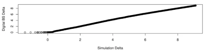
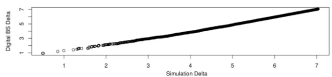
i.e., regressing the discounted payoffs at time T on state variables at time t. Fig-ures 10-12 are for the prices of a digital call option under Black-Scholes set-ting and Figures 13-15 are QQ-plots for Delta values. Figure 16 and Figure

17 show the QQ-plots for method 3 under Heston model with 3 nested ANN

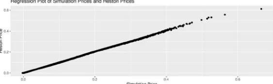
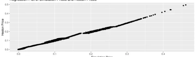
[image:11.595.231.517.238.325.2] [image:11.595.233.516.365.450.2]

approximations of size 4 and one ANN approximation of size 12 using R rou-tine nnet. The absolute RMSE for the former is 0.1938% and latter 0.2581%, with the running time 10.36 seconds compared to 52.31 for ANN approxima-tion with size 12.

[image:11.595.232.516.489.578.2]

Figure 1. QQ-plot for Method 1, τ=0.05 and relative pricing error is 1.20%.

[image:11.595.233.515.616.703.2]

(12)

[image:12.595.218.533.77.170.2] [image:12.595.220.531.211.302.2]

[image:12.595.219.527.342.438.2]

Figure 5. QQ-plot for Method 1, τ =0.20 and relative pricing error is 1.75%.

[image:12.595.217.531.478.570.2]

[image:12.595.219.532.610.704.2]

(13)

[image:13.595.216.540.81.180.2] [image:13.595.213.538.227.328.2]

[image:13.595.214.536.373.475.2]

Figure 13. Delta QQ-plot for Method 1, τ=0.02.

[image:13.595.206.541.506.714.2] [image:13.595.209.538.514.592.2] [image:13.595.208.539.623.708.2]

(14)

[image:14.595.209.540.56.365.2]

Figure 15. Delta QQ-plot for Method 1, τ=0.08.

Figure 16. Price QQ-plot for Method 3, τ=0.20.

Figure 17. Price QQ-plot for Method 3, τ=0.20.

4.2. American Option Pricing

Here we refer the readers to [67] for the BSDE satisfied by a plain vanilla Amer-ican option. For r=0.03, d =0.07, σ =0.20, T =3.00, N =150, S0 =100

and K=100_{, the benchmark American option price at}t₀ =0_{is 9.0660 and}

the relative difference of our Monte-Carlo price is 0.27%. The running time is less than 30 seconds.

5. Conclusion and Future Research

[image:14.595.206.539.65.142.2]

(15)

in the context of American game options, equity swaps, and the related

Mckean-Vlasov type FBSDEJs (mean-field FBSDEJ, see [70]) are important

top-ics in mathematical finance. They are also related to the theoretical analysis of high-frequency trading. Finding machine-learning based numerical methods to solve these equations is of great interest to us. Last, but not least, machine learn-ing methods in asset priclearn-ing and portfolio optimization, which can be found in

[71], [72], [73], [28], [74] and [75], admit an elegant way to price financial de-rivatives under -measure. For example, we can use the method in [72] to ca-librate the SDF process and use [75] to generate market scenarios. These me-thodologies, combined with the methods documented in this paper and [1], have the potential to solve for any derivative price. We leave all the development to future research.

Acknowledgements

We thank the Editor and the referee for their comments. Moreover, we are grateful to Professor Jérôme Detemple, Professor Marcel Rindisbacher and Pro-fessor Weidong Tian for their useful suggestions.

Conflicts of Interest

The authors declare no conflicts of interest regarding the publication of this pa-per.

References

[1] Longstaff, F. and Schwartz, E. (2001) Valuing American Options by Simulation: A Simple Least—Square Approach.TheReview of Financial Studies, 14, 113-147.

https://doi.org/10.1093/rfs/14.1.113

[2] El Karoui, N., Peng, S. and Quenez, M.C. (1997) Backward Stochastic Differential Equations in Finance. MathematicalFinance, 7, 1-71.

https://doi.org/10.1111/1467-9965.00022

[3] Adrian, T., Crump, R. and Vogt, E. (2018) Nonlinearity and Flight-to-Safety in the Risk-Return Trade-Off for Stocks and Bonds. Forthcoming in Journal of Finance, 74, 1931-1973.

[4] Fama, E. and French, K. (1993) Common Risk Factors in the Returns on Stocks and Bonds. Journal of Financial Economics, 33, 3-56.

https://doi.org/10.1016/0304-405X(93)90023-5

[5] Fama, E. and French, K. (2015) A Five-Factor Asset Pricing Model. Journal of Fi-nancialEconomics, 116, 1-22.

[6] Zhu, S. and Pykhtin, M. (2008) A Guide to Modeling Counterparty Credit Risk. Working Paper. https://papers.ssrn.com/sol3/papers.cfm?abstract_id=1032522 [7] Aydogdu, M. (2018) Predicting Stock Returns Using Neural Networks. Working

Paper. https://papers.ssrn.com/sol3/papers.cfm?abstract_id=3141492

https://doi.org/10.2139/ssrn.3141492

[8] Voshgha, H. (2008) Early Detection of Defaulting Firms: Artificial Neural Network Application; Australian Context. Working Paper.

(16)

DOI: 10.4236/jmf.2019.93029 576 Journal of Mathematical Finance [9] Hutchinson, J., Lo, A. and Poggio, T. (1994) A Nonparametric Approach to Pricing and Hedging Derivative Securities via Learning Networks. Journal of Finance, 49, 851-889.https://doi.org/10.1111/j.1540-6261.1994.tb00081.x

[10] Hahn, J.T. (2013) Option Pricing Using Artificial Neural Networks: The Australian Perspective. Ph.D. Thesis, Bond University, Queensland‎.

[11] Kohler, M., Krzyzak, M. and Todorovic, N. (2010) Pricing of High-Dimensional American Options by Neural Networks. MathematicalFinance, 20, 383-410.

https://doi.org/10.1111/j.1467-9965.2010.00404.x

[12] Dugas, C., Bengio, Y., Bélisle, F., Nadeau, C. and Garcia, R. (2009) Incorporating Functional Knowledge in Neural Networks. Journal of Machine Learning Research, 10, 1239-1262.

[13] Eckstein, S., Kupper, M. and Pohl, M. (2018) Robust Risk Aggregation with Neural Networks. QuantitativeFinance, 1-40. https://arxiv.org/abs/1811.00304

[14] Giovanis, E. (2010) Applications of Neural Network Radial Basis Function in Eco-nomics and Financial time Series. SSRN Electronic Journal.

https://papers.ssrn.com/sol3/papers.cfm?abstract_id=1667442

[15] Kopitkov, D. and Indelman, V. (2018) Deep PDF: Probabilistic Surface Optimiza-tion and Density EstimaOptimiza-tion. Computer Science, 1-18.

https://arxiv.org/abs/1807.10728

[16] Luo, R., Zhang, W., Xu, X. and Wang, J. (2017) A Neural Stochastic Volatility Mod-el. Computer Science, 1-11. https://arxiv.org/pdf/1712.00504.pdf

[17] Sasaki, H. and Hyvärinen, A. (2018) Neural-Kernelized Conditional Density Esti-mation. Statistics, 1-12. https://arxiv.org/abs/1806.01754

[18] Weissensteiner, A. (2009) AQ-Learning Approach to Derive Optimal Consumption and Investment Strategies. IEEETransactions on Neural Networks, 20, 1234-1243.

https://doi.org/10.1109/TNN.2009.2020850

[19] Casgrain, P. and Jaimungal, S. (2016) Trading Algorithms with Learning in Latent Alpha Models. SSRN Electronic Journal. https://doi.org/10.2139/ssrn.2871403 https://papers.ssrn.com/sol3/papers.cfm?abstract_id=2871403

[20] Heaton, J., Polson, N. and Witte, J. (2016) Deep Learning for Finance: Deep Portfo-lios. Applied Stochastic Models in Business and Industry, 33, 3-12.

https://papers.ssrn.com/sol3/papers.cfm?abstract_id=2838013 https://doi.org/10.2139/ssrn.2838013

[21] Samo, Y. and Vernuurt, A. (2016) Stochastic Portfolio Theory: A Machine Learning Perspective. Quantitative Finance, 1-9. https://arxiv.org/pdf/1605.02654.pdf

[22] Jiang, Z., Xu, D. and Liang, J. (2017) A Deep Reinforcement Learning Framework for the Financial Portfolio Management Problem. Computational Finance, 1-31.

https://arxiv.org/pdf/1706.10059.pdf

[23] Deng, Y., Bao, F., Kong, Y., Ren, Z. and Dai, Q. (2017) Deep Direct Reinforcement Learning for Financial Signal Representation and Trading. IEEE Transactions on Neural Networks and Learning Systems, 28, 653-664.

https://doi.org/10.1109/TNNLS.2016.2522401

[24] Halperin, I. (2017) QLBS: Q-Learner in the Black-Scholes(-Merton) Worlds. Quan-titativeFinance, 1-34. https://arxiv.org/abs/1712.04609v2

[25] Ritter, G. (2017) Machine Learning for Trading. Working Paper.

(17)

DOI: 10.4236/jmf.2019.93029 577 Journal of Mathematical Finance https://doi.org/10.2139/ssrn.3015609

[26] Xing, F., Cambrida, E., Malandri, L. and Vercellis, C. (2018) Discovering Bayesian Market Views for Intelligent Asset Allocatio. https://arxiv.org/pdf/1802.09911.pdf [27] Becker, S., Cheridito, P. and Jentzen, A. (2018) Deep Optimal Stopping.

Mathemat-ics, arXiv: 1804. 05394. https://arxiv.org/abs/1804.05394

[28] Gu, S., Kelly, B. and Xiu, D. (2018) Empirical Asset Pricing via Machine Learning. 31st Australasian Finance and Banking Conference 2018, Sydney, 13-15 December 2018. https://doi.org/10.3386/w25398

[29] Weinan, E., Han, J. and Jentzen, A. (2017) Deep Learning-Based Numerical Me-thods for High-Dimensional Parabolic Partial Differential Equations and Backward Stochastic Differential Equations. Mathematics, 1-39.

[30] Weinan, E., Hutzenthaler, M., Jentzen, A. and Kruse, T. (2017) On Multilevel Pi-card Numerical Approximations for High-Dimensional Nonlinear Parabolic Partial Differential Equations and High-Dimensional Nonlinear Backward Stochastic Dif-ferential Equations. Mathematics, 1-25. https://arxiv.org/pdf/1708.03223.pdf [31] Han, J., Jentzen, A. and Weinan, E. (2017) Overcoming the Curse of

Dimensionali-ty: Solving High-Dimensional Partial Differential Equations Using Deep Learning.

Mathematics, 1-14. https://arxiv.org/pdf/1707.02568.pdf

[32] Khoo, Y., Lu, J. and Ying, L. (2017) Solving Parametric PDE Problems with Artifi-cial Neural Networks. Mathematics, 1-17. https://arxiv.org/pdf/1707.03351.pdf [33] Beck, C., Weinan, E. and Jentzen, A. (2017) Machine Learning Approximation

Al-gorithms for High-Dimensional Fully Nonlinear Partial Differential Equations and Second-Order Backward Stochastic Differential Equations. Mathematics, 1-56.

[34] Sirignano, J. and Spiliopoulos, K. (2017) DGM: A Deep Learning Algorithm for Solving Partial Differential Equations. Mathematics, 1-31.

[35] Long, Z., Lu, Y. and Ma, X. (2018) PDE-Net: Learning PDEs from Data. Mathemat-ics, 1-17. https://arxiv.org/pdf/1710.09668.pdf

[36] Long, Z. and Lu, Y. (2018) PDE-Net 2.0: Learning PDEs from Data with a Numeric Symbolic Hybrid Deep Network. Computer Science, 1-16.

[37] Haehnel, P., Marecek, J. and Monteil, J. (2018) Scaling up Deep Learning for PDE-Based Models. Computer Science, 1-39. https://arxiv.org/pdf/1810.09425.pdf [38] Berg, J. and Nyström, K. (2018) Driven Discovery of PDEs in Complex

Data-sets. Statistics, 1-22. https://arxiv.org/pdf/1808.10788.pdf

[39] Rudy, S., Alla, A., Brunton, S. and Nathan Kutz, J. (2018) Data-Driven Identifica-tion of Parametric Partial Differential EquaIdentifica-tions. Mathematics, 1-17.

[40] Detemple, J., Lorig, M., Rindisbacher, M. and Zhang, L. (2018) An Analytical Ex-pansion Method for Forward Backwards to Chastic Differential Equations with Jumps.

[41] Briand, P. and Labart, C. (2012) Simulation of BSDEs by Wiener Chaos Expansion.

The Annals of AppliedProbability, 24, 1129-1171.

https://doi.org/10.1214/13-AAP943

(18)

DOI: 10.4236/jmf.2019.93029 578 Journal of Mathematical Finance Expansion.Mathematics, arXiv: 1502.05649. http://arxiv.org/abs/1502.05649 [43] Gnameho, K., Stadje, M. and Pelsser, A. (2017) A Regression-Later Algorithm for

Backward Stochastic Differential Equations. Mathematics, 1-33.

https://arxiv.org/pdf/1706.07986

[44] Gobet, E. and Labart, C. (2007) Error Expansion for the Discretization of Backward Stochastic Differential Equations. Stochastic Processes and Their Applications, 117, 803-829.https://doi.org/10.1016/j.spa.2006.10.007

[45] Takahashi, A. and Yamada, T. (2016) An Asymptotic Expansion for For-ward-Backward SDEs: A Malliavin Calculus Approach.Asia-Pacific Financial Mar-kets, 23, 337-373.

[46] Takahashi, A. and Yamada, T. (2015) On the Expansion to Quadratic FBSDEs. [47] Gobet, E. and Pagliarani, S. (2014) Analytical Approximations of BSDEs with

Non-Smooth Driver. SIAM Journal on Financial Mathematics, 6, 919-958.

[48] Fujii, M. and Takahashi, A. (2012) Analytical Approximation for Non-Linear FBSDEs with Perturbation Scheme. InternationalJournal of Theoretical and Ap-plied Finance, 15, Article ID: 1250034.https://doi.org/10.1142/S0219024912500343

[49] Fujii, M. and Takahashi, A. (2012) Perturbative Expansion of FBSDE in an Incom-plete Market with Stochastic Volatility. The Quarterly Journal of Finance, 2, 1-22.

[50] Fujii, M. and Takahashi, A. (2015) Asymptotic Expansion for Forward-Backward SDEs with Jumps. QuantitativeFinance, 1-39. https://doi.org/10.2139/ssrn.2672890

[51] Fujii, M. and Takahashi, A. (2016) Quadratic-Exponential Growth BSDEs with Jumps and Their Malliavin’s Differentiability. Working Paper.

http://papers.ssrn.com/sol3/papers.cfm?abstract_id=2705670

[52] Fujii, M. and Takahashi, A. (2016) Solving Backward Stochastic Differential Equa-tions by Connecting the Short-Term Expansions. QuantitativeFinance, 1-41.

[53] Detemple, J. and Rindisbacher, M. (2005) Closed-Form Solutions for Optimal Portfolio Selection with Stochastic Interest Rate and Investment Constraints. Ma-thematicalFinance, 15, 539-568.https://doi.org/10.1111/j.1467-9965.2005.00250.x

[54] Hansen, L. and Richard, S. (1987) The Role of Conditioning Information in De-ducing Testable Restrictions Implied by Dynamic Asset Pricing Models. Econome-trica, 55, 587-613.https://doi.org/10.2307/1913601

[55] Jiang, J. and Tian, W. (2018) Semi-Nonparametric Approximation and Index Op-tions. Annals of Finance, 1-38.https://doi.org/10.1007/s10436-018-0341-4

[56] Tian, W. (2014) Spanning with Indexes. Journal of Mathematical Economics, 53, 111-118.https://doi.org/10.1016/j.jmateco.2014.06.007

[57] Tian, W. (2018) The Financial Market: Not as Big as You Think. Mathematics and FinancialEconomics, 51, 1-19.

[58] Bölcskei, H., Grohs, P., Kutyniok, G. and Petersen, P. (2018) Optimal Approxima-tion with Sparsely Connected Deep Neural Networks. ComputerScience, 1-36.

[59] Henry-Labordere, P. (2015) Exact Simulation of Multi-Dimensional Stochastic Dif-ferential Equations. Working Paper, 1-28. https://doi.org/10.2139/ssrn.2598505

(19)

DOI: 10.4236/jmf.2019.93029 579 Journal of Mathematical Finance [60] Prater, A. (2012) Discrete Sparse Fourier Hermite Approximations in High

Dimen-sions. Doctoral Thesis, Syracuse University,New York.

[61] Fonseca, Y., Medeiros, M., Vasconcelos, G. and Veiga, A. (2018) Boost: Boosting Smooth Trees for Partial Effect Estimation in Nonlinear Regressions. Statistics, 1-30. https://arxiv.org/pdf/1808.03698.pdf

[62] Detemple, J. (2006) American-Style Derivatives: Valuation and Computation. Chapman and Hall/CRC, New York.https://doi.org/10.1201/9781420034868

[63] Guyon, J. and Henry-Labordere, P. (2014) Nonliner Option Pricing. Chapman and Hall, New York.https://doi.org/10.1201/b16332

[64] Detemple, J., Garcia, R. and Rindisbacher, M. (2005) Representation Formulas for Malliavin Derivatives of Diffusion Processes. Finance and Stochastics, 9, 349-367.

https://doi.org/10.1007/s00780-004-0151-6

[65] Detemple, J. and Rindisbacher, M. (2005) Asymptotic Properties of Monte Carlo Estimators of Derivatives. ManagementScience, 51, 1657-1675.

https://doi.org/10.1287/mnsc.1050.0398

[66] Detemple, J. (2014) Optimal Exercise for Derivative Securities. Annual Review of FinancialEconomics, 6, 459-487.

https://doi.org/10.1146/annurev-financial-110613-034241

[67] Fujii, M., Sato, S. and Takahashi, A. (2012) An FBSDE Approach to American Op-tion Pricing with an Interacting Particle Method. Quantitative Finance, 1-18.

[68] Chassagneux, J., Elie, R. and Kharroubi, I. (2010) A Note on Existence and Unique-ness for Solutions of Multidimensional Reflected BSDEs. Electronic Communica-tions in Probability, 16, 120-128.https://doi.org/10.1214/ECP.v16-1614

[69] Collin-Dufresne, P. and Goldstein, R. (2003) Generalizing the Affine Framework to HJM and Random Field Models. SSRN Electronic Journal.

[70] Carmona, R. and Delarue, F. (2015) Forward-Backward Stochastic Differential Eq-uations and Controlled McKean-Vlasov Dynamics. Annals of Probability, 43, 2647-2700.https://doi.org/10.1214/14-AOP946

[71] Bianchi, D., Büchner, M. and Tamoni, A. (2019) Bond Risk Premia with Machine Learning. USC-INET Research Paper No. 19-11.

[72] Chen, L., Pelger, M. and Zhu, J. (2019) Deep Learning in Asset Pricing. Quantitative Finance, 1-89. https://arxiv.org/abs/1904.00745

[73] Feng, G., Polson, N. and Xu, J. (2019) Deep Learning in Asset Pricing. Statistics, 1-33. https://papers.ssrn.com/sol3/papers.cfm?abstract_id=3350138

[74] Yang, Q., Ye, T. and Zhang, L. (2018) A General Framework of Optimal Invest-ment. Working Paper.

[75] Yu, P., Lee, J., Kulyatin, I., Shi, Z. and Dasgupta, S. (2019) Model-Based Deep Rein-forcement Learning for Dynamic Portfolio Optimization. ComputerScience, 1-21.

(20)

ComputerScience, 1-15. https://arxiv.org/abs/1412.6980

[77] Heston, S. (1993) A Closed-Form Solution for Options with Stochastic Volatility with Applications to Bond and Currency Options. TheReview of Financial Studies, 6, 327-343.https://doi.org/10.1093/rfs/6.2.327

[78] Dupire, B. (1994) Pricing with a Smile. Risk.

http://www.risk.net/data/risk/pdf/technical/2007/risk20_0707_technical_volatility.p df

[79] Homescu, C. (2014) Local Stochastic Volatility Models: Calibration and Pricing. Working Paper. https://papers.ssrn.com/sol3/papers.cfm?abstract_id=2448098

[80] Broadie, M., Chernov, M. and Johannes, M. (2007) Model Specification and Risk Premia: Evidence from futures Options. Journal of Finance, 62, 1453-1490.

https://doi.org/10.1111/j.1540-6261.2007.01241.x

[81] Guennon, H. (2016) Local Volatility Models Enhanced with Jumps. Working Paper, 1-11. https://papers.ssrn.com/abstract=2781102

[82] Buehler, H., Gonon, L., Teichmann, J. and Wood, B. (2018) Deep Hedging. Work-ing Paper. https://doi.org/10.2139/ssrn.3120710

[83] Halperin, I. (2018) The QLBS Q-Learner Goes NuQLear: Fitted Q Iteration, Inverse RL, and Option Portfolios. QuantitativeFinance, 1-18.

[84] Halperin, I. (2018) QLBS: Q-Learner in the Black-Scholes(-Merton) Worlds. Quan-titativeFinance, 1-34. https://arxiv.org/abs/1712.04609

[85] Schroder, M. and Skiadas, C. (2008) Optimality and State Pricing in Constrained Financial Markets with Recursive Utility under Continuous and Discontinuous In-formation. MathematicalFinance, 18, 199-238.

https://doi.org/10.1111/j.1467-9965.2007.00330.x

[86] Detemple, J. and Zapatero, F. (1991) Asset Prices in an Exchange Economy with Habit Formation. Econometrica, 59, 1633-1657.https://doi.org/10.2307/2938283

[87] Karatzas, I., Lehoczky, J., Shreve, S. and Xu, G. (1991) Martingale and Duality Me-thods for Utility Maximization in a Incomplete Market. SIAMJournal on Control and Optimization, 29, 702-730.https://doi.org/10.1137/0329039

[88] He, H. and Pearson, N. (1991) Consumption and Portfolio Policies with Incomplete Markets and Short-Sale Constraints: The Infinite Dimensional Case. Journal of EconomicTheory, 54, 259-304.https://doi.org/10.1016/0022-0531(91)90123-L

[89] Karatzas, I. and Cvitanic, J. (1992) Convex Duality in Constrained Portfolio Opti-mization. Annals of Applied Probability, 2, 767-818.

https://doi.org/10.1214/aoap/1177005576

[90] Detemple, J., Garcia, R. and Rindisbacher, M. (2003) A Monte Carlo Method for Optimal Portfolios. Journal of Finance, 58, 401-446.

https://doi.org/10.1111/1540-6261.00529

[91] Detemple, J., Garcia, R. and Rindisbacher, M. (2005) Intertemporal Asset Alloca-tion: A Comparison of Methods. Journal of Banking and Finance, 29, 2821-2848.

https://doi.org/10.1016/j.jbankfin.2005.02.004

(21)

De-DOI: 10.4236/jmf.2019.93029 581 Journal of Mathematical Finance composition Formula and Applications. The Review of Financial Studies, 23, 25-100. https://doi.org/10.1093/rfs/hhp040

[93] Detemple, J. (2012) Portfolio Selection: A Review. Journal of Optimization Theory andApplications, 161, 1-21.https://doi.org/10.1007/s10957-012-0208-1

[94] Matoussi, A. and Xing, H. (2016) Convex Duality for Stochastic Differential Utility.

Quantitative Finance, 1-22. http://arxiv.org/pdf/1601.03562.pdf https://doi.org/10.2139/ssrn.2715425

[95] Kraft, H., Seiferling, T. and Seifried, F. (2015) Optimal Consumption and Invest-ment with Epstein-Z in Recursive Utility. Working Paper.

[96] Aït-Sahalia, Y. (2008) Closed-Form Likelihood Expansions for Multivariate Diffu-sions. Annals of Statistics, 36, 906-937.

https://doi.org/10.1214/009053607000000622

[97] Filipović, D., Mayerhofer, E. and Schneider, P. (2013) Density Approximations for Multivariate Affine Jump Diffusion Processes. Journal of Econometrics, 176, 93-111. https://doi.org/10.1016/j.jeconom.2012.12.003

[98] Van Handel, R. (2008) Hidden Markov Models. Princeton Lecture Notes. [99] Markowitz, H. (1952) Portfolio Selection. Journal of Finance, 7, 77-91.

https://doi.org/10.1111/j.1540-6261.1952.tb01525.x

[100]Schneider, P. and Trojani, F. (2018) (Almost) Model Free Recovery. Forthcomingin Journal of Finance, 74, 323-370.https://doi.org/10.1111/jofi.12737

[101]Chabakauri, G. (2013) Dynamic Equilibrium with Two Stocks, Heterogeneous In-vestors, and Portfolio Constraints.The Review of Financial Studies, 26, 3104-3141.

[102]Chabakauri, G. (2015) Asset Pricing with Heterogeneous Preferences, Beliefs, and Portfolio Constraints.Journal of Monetary Economics, 75, 21-34.

[103]Kardaras, C., Xing, H. and Žitković, G. (2015) Incomplete Stochastic Equilibria for Dynamic Monetary Utility. Mathematics, 1-33. https://arxiv.org/abs/1505.07224 [104]Halle, J.O. (2010) Backward Stochastic Differential Equations with Jumps. Master

Thesis, University of Oslo, Oslo, Norway.

(22)

Appendix

A. Convergence of the Proposed Methodologies

Proof of Theorem 10. It is known from the projection theorem of Hilbert space that

{ }

hn n 1

∞

= and h actually exist and are unique. Moreover, PROJnh h= n as indicated by the repeated projection theorem. It is also known that

ORTH _n

n

h h− ∈ _ . As we ask that Assumption 6 hold, we know that

0

n

h h− _ → +_as

n

→ ∞

_.

Proof of Theorem 12. The proof follows from Assumption 6 and Theorem 8. We have

lim PROJ _n

n→∞ Ψ x (27)

lim PROJ _nPROJ _n

n→∞ Ψ x

= __ _ (28)

lim PROJ _n n

n→∞ Ψ h

= __ (29)

PROJΨ h

= __ ₍₃₀₎

.

h

= (31)

This concludes the proof.

Proof of Lemma 1. For any 2

( )

t L t

λ

∈  , we have

(

)

2

T t

ξ λ

 ₋ 

 

 (32)

[ ]

(

)

2

(

[ ]

)

2

T t T t t T

ξ

λ

ξ

   

=__ − __+__ − __ (33)

[ ]

(

)

(

[ ]

)

0

2 λt t ξT ξT t ξT

=

 

+ _ − − _

    (34)

[ ]

(

)

2

(

[ ]

)

2

T t T t t T

ξ

λ

ξ

   

=___ −_ __+___ −_ __₍₃₅₎

[ ]

(

)

2

.

T t T

ξ

 

≥__ − __ (36)

Therefore we have the claim announced.

Proof of Theorem 17. The proof of this theorem follows from Assumptions 1, 2, 6, 14, 15 and Theorem 10, by choosing

[ ]

( )

[ ]

( )

{

_| 2 _, 2

}

2

( )

2

( )

t

ξ

T

ξ

T∈L T t

ξ

T ∈L t ⊂ t ⊂L t ⊂L T = T

        .

Proof of Theorem 18. Essentially, Equation (7) is the result of Gauss-Markov Theorem and the consistency property of OLS estimator.

Proof of Proposition 19. This is a direct consequence of the discussion in ([57], Section 3) (see Equation (5)) and Theorem 10. To elaborate, consider

( )

2

T =L T

  , x=ψ

( )

XT , its projections h and hn on 1 2

( )

n

t _n t L t

∞ =

=

_

⊂

  

and n

t

 defined in this proposition. Suppose that

1

j j t j

h ∞

λ

e

=

∑

_and mn₁ n j

n j j t

h =

∑

₌

µ

e _,

where mn <mn+1 and

{ }

etj _j₁ ∞

= is a set of orthonormal basis in t. From the

repeated projection theorem, we know that n 1 n

j j j

µ

+ ₌

µ

₌

λ

_{for any}₁

n

j m

≤ ≤ 6

6_{Here we only consider the case where}

n mn

Λ = < ∞ for any n∈. The case with Λ = ∞n is