doi:10.4236/ojs.2011.11001 Published Online April 2011 (http://www.SciRP.org/journal/ojs)
Modified
C
p
Criterion for Optimizing Ridge and Smooth
Parameters in the MGR Estimator for the Nonparametric
GMANOVA Model
Isamu Nagai
Department of Mathematics, Graduate School of Science, Hiroshima University 1-3-1 Kagamiyama, Higashi-Hiroshima, Hiroshima 739-8626, Japan
E-mail: [email protected]
Received March 18, 2011; revised April 2, 2011; accepted April 12, 2011
Abstract
Longitudinal trends of observations can be estimated using the generalized multivariate analysis of variance (GMANOVA) model proposed by [10]. In the present paper, we consider estimating the trends nonparamet-rically using known basis functions. Then, as in nonparametric regression, an overfitting problem occurs. [13] showed that the GMANOVA model is equivalent to the varying coefficient model with non-longitudinal covariates. Hence, as in the case of the ordinary linear regression model, when the number of covariates be-comes large, the estimator of the varying coefficient bebe-comes unstable. In the present paper, we avoid the overfitting problem and the instability problem by applying the concept behind penalized smoothing spline regression and multivariate generalized ridge regression. In addition, we propose two criteria to optimize hyper parameters, namely, a smoothing parameter and ridge parameters. Finally, we compare the ordinary least square estimator and the new estimator.
Keywords:Generalized ridge regression, GMANOVA model, Mallows' Cpstatistic, Non-iterative estimator,
Shrinkage estimator, Varying coefficient model
1. Introduction
We consider the generalized multivariate analysis of vari-ance (GMANOVA) model withnobservations of
p-dimensional vectors of response variables. This model was proposed by [10]. Let Y
y1,,yn
', A, X and
1, , n
'
Ε ε ε be an np matrix of response vari- ables, an n k matrix of non-stochastic centerized be-tween-individual explanatory variables (i.e., A 1n 0k)
of rank
A k (n), a p q matrix of non-stochastic within-individual explanatory variables of rank
X q
q p
, and an np matrix of error variables, respec-tively, wherenis the sample size, 1nis an n-dimensionalvector of ones and 0k is a k-dimensional vector of zeros.
Then, the GMANOVA model is expressed as
n
Y 1 X + A X + EΞ
where Ξ
ξ1,,ξk
' is a k q unknown regressioncoefficient matrix an μ is q-dimensional unknown vec-tor. We assume that ε1,,εn i.i.d. Np
0p,Σ
where Σis a pp unknown covariance matrix of rank
Σ p. Then we can express the GMANOVA model as
,
n p n n
Y N 1 X A XΞ Σ I
Let S be an unbiased estimator of the unknown co-variance matrix Σ that is given by
1
1
n n n n n k
S = Y I 1 1 A A A A Y
Then, the maximum likelihood (ML) estimators of μ and Ξ are given by n1
1
1 1 n
X S X X S Y 1
and
1
11 1
A A A YS X X S X , respectively. The ML es-timators are the unbiased and asymptotically efficiency estimators of μ and Ξ.
In the GMANOVA model, x
t
1, ,t,tq1
',
tt1,,tp
is often used as the jth row vector of X. Then, we estimate the longitudinal trends of Y usingpolynomial curve cannot thoroughly express flexible lon-gitudinal trends. Hence, we consider estimating the longi-tudinal trends nonparametrically in the same manner as [11] and [5], i.e., we use the known basis function as x
tand assume that p is large. In the present paper, we refer to the GMANOVA model with X obtained from the basis function as the nonparametric GMANOVA model. In the nonparametric GMANOVA model, it is well known that the ML estimators become unstable because S1 becomes unstable when p is large. Thus, we deal with the least square (LS) estimators of μ and Ξ, which are o b t a i n e d b y m i n i m i z i n g tr
Y 1 nμ X AΞX
Y 1 nμ X AΞX
'
. Then, the LS estimators of μ and Ξ are obtained by μˆ n1(X X )1X Y 1n and
1
1 ˆ A A A YX X X Ξ respectively. Note that ˆμ does not depend on A. The LS estimators are simple and unbiased estimators of μ and Ξ. However, as well as ordinary nonparametric regression model, the LS estima-tors cause an overfitting problem when we use basis func-tions to estimate the longitudinal trends nonparametrically. In order to avoid the overfitting problem, we use
X X K instead of X X as the penalized smoothing spline regression (see, e.g., [2]), where
0 is a smoothing parameter and K is a q q known penalty matrix.Let i
y ti
1 , y ti
p
y , and let
1 , ,
i i t i tp
ε ε ε . Then, the GMANOVA model can be expressed as
1 1
' ' ,
1, , ; , , , k
i ij j i
j
p
y t t a t t
i n t t t
x μ x
ξ
where aij is the
i j, th element of A. This expressionindicates that the GMANOVA model is equivalent to the varying coefficient model with non-longitudinal covariates [13], i.e.,
0
1 1
,
1, , ; , , , k
i ij j i
j
p
y t t a t t
i n t t t
(4)
where 0
t x
t 'μ and j
t x
t 'ξj ,
j1,,k
. Hence, estimating the longitudinal trends in the GMANOVA model nonparametrically is equivalent to estimating the varying coefficients j
t ,
j0,,k
nonparametrically. However, when multicollinearity occurs
in A, the estimate of j
t ,
j1,,k
becomesunstable, as does the ordinary LS estimator of regression coefficient, because the variance of an estimator of j
tbecomes large. Hence, we avoid the multicollinearity problem in A by the ridge regression.
When X Ιp and p1 in the model (1), [4]
pro-posed a ridge regression. This estimator is generally de-fined by adding Ik to A A in (3), where 0 is
referred to as a ridge parameter. Since the ridge estimator changes with , optimization of is very important. One method for optimizing is minimizing the Cp
criterion proposed by [7,8] in the univariate linear regres-sion model (for multivariate case, see e.g., [15]). For the case in which XΙp and p1, [17] proposed the Cp and its bias-corrected Cp (modified Cp; MCp) criteria for optimizing the ridge parameter. However, an optimal
cannot be obtained without an iterative computational algorithm because an optimal cannot be obtained in closed form.
On the other hand, [4] also proposed a generalized ridge (GR) regression in the univariate linear regression model, i.e., the model (1) with X Ιp and p1,
simultane-ously with the ridge regression. The GR estimator is de-fined not by a single ridge parameter, but rather by multiple ridge parameters θ
1,,k
',
i 0, i1,,k
.Then, several authors proposed a non-iterative GR estima-tor (see, e.g., [6]). [18] proposed a GR regression in the multivariate linear regression model, i.e., the model (1) with X Ιp and p1. We call this generalized ridge
regression the multivariate GR (MGR) regression. They also proposed the Cp and MCp criteria for optimizing
ridge parameters θ in the MGR regression. They showed that the optimized θ by minimizing two criteria are ob-tained in closed form. [9] proposed non-iterative MGR estimators by extending non-iterative GR estimators. Sev-eral computational tasks are required in estimating j
tnonparametrically because we determine the optimal and the number of basis functions simultaneously. Fortu-nately, [18] reported that the performance of the MGR re-gression is the almost same as that of the multivariate ridge regression. Hence, we use the MGR regression in order to avoid the multicollinearity problem that occurs in A in order to reduce the number of computational tasks.
The remainder of the present paper is organized as fol-lows: In Section 2, we propose new estimators using the concept of the penalized smoothing spline regression and the MGR regression. In Section 3, we show the target mean squared error (MSE) of a predicted value of Y . We then propose the Cp and MCp criteria to optimize ridge
Using these criteria, we show that the optimized ridge pa-rameters are obtained in closed form under the fixed . We also show the magnitude relationship between the op-timized ridge parameters. In Section 4, we compare the LS estimator in (3) with the proposed estimator through nu-merical studies. In Section 5, we present our conclusions.
2. The New Estimators
In the model (1), we consider estimating the longitudinal trends nonparametrically by using basis functions X . Then, we consider the following estimators in order to avoid the overfitting problem in the nonparametric GMANOVA model, ˆ 1
1n
n
μ X X K X Y1 and
,1 ,
1 1
ˆ ˆ
ˆ , , '
k
A A A YX X X K
Ξ ξ ξ
(5)
where
0 is a smoothing parameter and Kis a q q known penalty matrix. In this estimator, we must determine K before using this estimator. Since K is usually set as some nonnegative definite matrix, we as-sume that K is a nonnegative definite matrix. If,
q q
KO , whereOq q, is a q q matrix of zeros, then this estimator corresponds to the LS estimators μˆ and
ˆ
Ξ in (1). Note that this estimator controls the smooth-ness of each estimated curve ˆ0
t x
t 'μˆ and
ˆ ,ˆ '
j t t j
x ξ ,
j1,,k
through only one pa-rameter . When we use this estimator, we need to op-timize the parameter because this estimator changes with.If multicollinearity occurs in A, then the LS estima-tor Ξˆ in (1) and the proposed estimator Ξˆ in (5) are not good estimators in the sense of having large variance. Note that neither the LS estimator μˆ nor the proposed estimator ˆμ depend on A. Hence, we avoid the mul-ticollinearity problem for estimating Ξ. Multicollinear-ity often occurs when k becomes large. Using the fol-lowing estimator, the multicollinearity problem in A can be avoided,
,1 ,
1 1
ˆ ˆ
ˆ , , '
( )
k
k
A A I A YX X X K
Ξ ξ ξ
(6)
where 0 is a ridge parameter. This estimator with
q
K I corresponds to the estimator of [16]. If 0, then this estimator corresponds to the estimator in (5). Note that
k
1
A A I A Y in this estimator corre-sponds to the ridge estimator for a multivariate linear model [17]. In this estimator, we need to optimize and because this estimator changes with these
pa-rameters. However, we cannot obtain the optimized and in closed form. Thus, we need to use an iterative computational algorithm to optimize two parameters. From another point of view, this estimator controls the smoothness of each estimated curve ˆj x
t 'ξˆ,j,
j1,,k
through only one parameter . Hence, this estimator is not a well fitting curve when the smoothnesses of the true curves differ.Hence, we apply the concept of the MGR estimator [18] to
k
1
A A I A Y in order to obtain the opti-mized ridge parameter in closed form. Here, we derive the MGR estimator for the nonparametric GMANOVA model as follows:
1
1,
ˆ
A A Q Q A YX X X K θ
Ξ Θ (7)
where θ
1,,k
',(i0,i1,..., )k is also a ridge parameter, Θdiag
θ , and Q is the k k or-thogonal matrix that diagonalizes A A , i.e.,
Q A AQ D where Ddiag
d1,,dk
and1, , k
d d are eigenvalues of A A . It is clearly that 0
i
d ,
i1,,k
. In this estimator, since θ shrinks the estimators of j
t ,
j1,,k
to 0, we canre-gard θ as controlling the smoothness of
1 t , , k t
. Therefore, in this estimator, rough smoothness of the estimated curves is controlled by , and each smoothness of j
t ,
j1,,k
iscon-trolled by θ.
Clearly, Ξˆ0k,0 Ξˆ and ,
ˆ ˆ
k
0
Ξ Ξ . The Ξˆθ, with
k
θ 1 for some
0 corresponds to Ξˆ , in (6). Thus, the estimator Ξˆθ, includes these estimators. The estimator Ξˆθ,is more flexible than these estimatorsˆ
Ξ and Ξˆ , because Ξˆθ, has k1 parameters and ˆ
Ξ or Ξˆ , has only one or two parameters. Hence, we consider μˆ and Ξˆθ, in estimating the longitudinal trends or the varying coefficient curve, while avoiding the overfitting and multicollinearity problems in the nonparametric GMANOVA model. When X Ιp and
,
q q
K O , Ξˆθ, corresponds to the MGR estimator in [18].
3. Main Results
3.1. Target MSE
Y , we prepare the following discrepancy function for measuring the distance between np matrices F1 and
1
1, 2 tr 1 2 1 2 '
r F F F F Σ F F : Since Σ is an unknown covariance matrix, we use the unbiased estimator S in (2) instead of Σ to estimate r
F F1, 2
. Hence, we estimate r
F F1, 2
using the following sample discrepancy function:
1
1 2 1 2 1 2
ˆ , tr '
r F F F F S F F (8) These two functions, r
F F1, 2
andrˆ
F F1, 2
,cor-respond to the summation of the Mahalanobis distance and the sample Mahalanobis distance between the rows of F1 and F2, respectively. Clearly, r
F F1, 2
2, 1
r F F and rˆ
F F1, 2
rˆ F F2, 1
. Through simplecalculation, we obtain the following properties:
1 2 3 1 3 2 ,
1
1 3 2
, , ,
2tr ,
n p
r r r
F F F F F F
F F F
O Σ
1 2 3 1 3 2 ,
1
1 3 2
ˆ , ˆ , ˆ ,
2tr{ },
n p
r r r
F F F F F F
F F S F
O
for any np matrices F1, F2 and F3, Using the discrepancy function r, the MSE of the predicted value of Y is defined as
, ,
ˆ ˆ
MSE E r E , ,
θ
Y Y Yθ (9)
where Yˆθ, 1nμˆ X AΞˆθ,X, which is the predicted value of Y when we use μˆ and Ξˆθ, in (7). In the present paper, we regard θ and making the MSE the smallest as the principle optimum. However, we cannot use the MSE in (9) in actual application because this MSE includes unknown parameters. Hence, we must estimate (9) in order to estimate the optimum θ and .
3.2. The Cp and MCp Criteria
Let H A A A Q Qθ
Θ
1A and
1
G X X X K X .
Note thatY E
Y E. Hence, we obtain
, ,
ˆ ˆ
MSEYθ E r Y E Y , θ .
From the properties of the functionr and using
1
1
tr tr
E YΣE E EΣ E , since E
Y is a nonstochastic variable and E
E On p, , and
4
4
tr tr
E F E F for any square matrix F4, we obtain
, , , 1 , 1 , 1 1 , 1 , 1 , ˆ ˆMSE , ,
ˆ 2 tr ˆ , tr 2 tr ˆ 2 tr ˆ , tr ˆ
2 tr .
n p
E r E r
E
E r E
E
E
E r E
E θ θ θ θ θ θ θ
Y Y Y E O
Y Y E
Y Y E E
Y E
Y E
Y Y E E
Y E Σ Σ Σ Σ Σ Σ
Note that ˆ,
n 1 n n
E
θ θ
Y 1 1 H Y E G .Thus,
we can calculate
1
, ˆ trE YθΣE as follows:
1 , 1 1 1 1 ˆ tr tr tr , n n n n EE n E
n E θ θ θ Y E
H Y E G E
H EG E
Σ
1 1 Σ
1 1 Σ
because E
Y , G and Σ1are non-stochastic variables. For calculating the expectations in the MSE, we prove the following lemma.
Lemma 3.1. For any pp non-stochastic matrix J, we obtain 1
tr n
EEJΣE J I .
proof. Since E
ε1,,εn
', we obtain the
i j, thelement of EEJΣ1E asE i 1 j
εJΣ ε ,
i1,, ;n
1, ,
j n . We obtainEε εi j i j, Σ becauseεi εj
for any i j and Cov
εi Σ for any i, where i j, is defined as i j, 1 if i j and i j, 0 if i j. Hence we obtain E i 1 j
εJΣ ε tr
i j, 1
JΣ Σ
, tr i j
J . This result means that E i 1 j tr
εJΣ ε J
if i j and 1 0
i j
EεJΣε if i j . Thus, the lemma is proven.
Using this lemma, we obtain
1
trE EΣE np
and
1
tr tr n
E EGΣE G I . Hence, we obtain
, , 1 , 1 , ˆ ˆ MSE , 2tr tr ˆ , 2tr tr ˆ, 2tr 1 tr
n n n
n n
E r np
n
E r np
n
E r np
θ θ θ θ θ θ θ
Y Y Y
H G I
Y Y
G H
Y Y G H
1 1
By replacing E r
Y Y,ˆθ,
with rˆ
Y Y,ˆθ,
, we can propose the instinctive estimator of MSE, referred to as the Cp criterion, as follows:
, ˆ
,ˆ,
2tr
tr 1 .
p
C θ r Y Yθ np G Hθ (10) When we use this criterion, we optimize the ridge pa-rameter θ and the smoothing parameter by the following algorithm:
1) We obtain θˆ(C)
arg minθCp
θ, , where
(C) (C) (C)
1
ˆ ˆ , ,ˆ '
k
θ
ˆ(C) 0, 1, ,
i i k
if is given.
2) We obtain ˆ(C)arg min0Cp
θˆ(C)
,
.3) We obtain ˆ(C)
ˆ(C) arg min
,ˆ(C)
pC
θ θ θ ,
where (C)
C
(C)
(C) (C)
(C)
1ˆ ˆ ˆ ˆ , ,ˆ ˆ '
k
θ ,
ˆ(C) ˆ(C)
0, 1, ,
i i k
under fixed ˆ(C).
4) We optimize the ridge parameter and the smoothing parameter as θˆ C
ˆ C and ˆ C , respectively.Note that this Cp criterion corresponds to that in [18]
when X Ip and K Oq q, .
There is some bias between the MSE in (9) and the
p
C criterion in (10) because the Cp criterion is
ob-tained by replacing E r
Y Y,ˆθ,
in the MSE withrˆ
Y Y,ˆθ,
. Generally, when the sample size n is small or the number of explanatory variables k is large, this bias becomes large. Then, we cannot obtain the high-er-accuracy estimation of the optimum parameters be-cause we cannot obtain the higher-accuracy estimation of MSE of Yˆθ,in (9). Hence, we correct the bias between, ˆ
MSEYθ and the Cpcriterion. To correct the bias,
we assume n k p 2 0.
LetW
n k 1
Sand Wθ,
Y Y ˆθ,
' Y Y ˆθ,
.
1
, ,
ˆ
, 1 [tr p .
E r n k E
Y Yθ Wθ W W I
Note thatW Wp
n k 1,Σ
andWθ,W 1
W because A 1n 0k and
1
, ( )
n k p
A I A A A A O .
Then, we obtain
Since EW1 Σ1/
n k p 2
, E
W
n k 1
Σ (see, e.g., [14]) and
1
,tr EWθΣ
,ˆ,
E r Y Yθ , we obtain
,
1 ,
,
ˆ ˆ ,
1
tr 2
2
1 ˆ
, 1
2
p
E r
n k
E n k p
n k p n k
E r p p
n k p
θ
θ
Y Y
W W I
θ
Σ Y Y
Therefore, we obtain the unbiased estimator for
,ˆ,
E r Y Yθ as c rMˆ
Y Y,ˆθ,
p p
1
, where
M 1 1 / 1
c p n k . This implies that the bias correctedCpcriterion, denoted as MCp(modifiedCp)
criterion, is obtained by
Mˆ ˆ,
, , 1
2tr tr 1 .
p
MC c r p p n
θ θ
θ Y Y
G H
(11)
As in the case of using theCp, we optimize θ and using this criterion as follows:
1) We obtainθˆ(M)
arg minθMCp
θ, , where
(M) (M ) (M)
1
ˆ ˆ , ,ˆ '
k
θ ,
ˆ(M ) 0, 1, ,
i i k
if is given.
2) We obtain ˆ( M) arg min0MCp
θˆ(M )
,
.3) We obtain ˆ(M)
ˆ(M)
ˆ(M )
arg min MCp ,
θ
θ θ ,
where (M )
(M )
(M )
(M ) (M)
(M)
1ˆ ˆ ˆ ˆ , ,ˆ ˆ '
k
θ ,
ˆ(M) ˆ(M)
0, 1, ,
i i k
under fixed ˆ(M).
4) We optimize the ridge parameter and the smoothing parameter as θˆ(M)
ˆ(M) and ˆ(M) , respectively.Note that the MCpcriterion corresponds to that in
[18] when XIp and KOq q, . The MCpcriterion completely omits the bias between the MSE of Yˆθ, in (9) and the Cp criterion in (10) by using a number of
constant terms cM and p p
1
. If θˆ(C)
and
(M)
ˆ
θ can be expressed in closed form for any fixed 0
, we do not need the above iterative computational algorithm.
3.3. Optimizations using the CpandMCpCriteria
given in (14), we can express the Cp and MCp
crite-ria as follows:
M
, , | 1 2tr ,
, , | 2tr 1
p p
p p
C GC np
MC GC c p p n
θ θ G
θ θ G
Note that the terms with respect to θ in the Cp and p
MC criteria correspond to GCp
θ,| 1
and
, | M
p
GC θ c , respectively. Hence, we consider ob-taining the optimum θ by minimizing the GCp crite-rion. From Theorem A, the optimum θ is obtained in closed form as (15). Using the closed form in (15), we obtain ˆ(C)
i
and ˆ(M)
i
for each i1,,k
and
any fixed 0 as follows:
C G
C
C
C C
C
ˆ ˆ | 1
0 0
( 0 ) ,
otherwise
i i
i
i i
i i ii
i ii
t d t
t t u
t u
(12)
M (G)
M M (M)
M M
M (M)
M
ˆ ˆ ( | )
0 (0 )
0 ,
otherwise
i i
i
i i
i i ii
i ii
c t
d t
t t c u
t c u
(13) where uii and vii are the
i i, th elements of1
Q A YG S G Y AQ and Q A YS G Y AQ 1 , respec-tively, (C)
| 1 - tr
i i ii ii i
t t v u d G and
(M)
M M
| - tr
i i ii ii i
t t c c v u d G . Note that
ii
u and vii vary with . Since
(C) ˆ
θ and
(M)
ˆ
θ are regarded as a function of , we can re-gard the Cp and MCp criteria for optimizing θ and
in (10) and (11) as a function of . This means that we can use these criteria to optimize.
Then, we can rewrite the optimization algorithms to optimize the ridge parameter θ and the smoothing parameter by minimizing the Cp and MCp
crite-ria in (10) and (11) as follows:
1) We obtainˆ(C) arg min0Cp
θˆ(C)
,
and
(M) (M )
0
ˆ arg min ˆ ,
p
MC
θ .
2) We optimize the ridge parameter and the smoothing parameter as θˆ(C)
ˆ(C) and θˆ(M )
ˆ(M) , respectively, by using ˆ(C), ˆ(M) and the closed forms in (12) and (13).This means that we can reduce the processing time to optimize the parameters, and we need to use the optimi-zation algorithm for only one parameter, , for any k.
3.4. Magnitude Relationships between Optimized Ridge Parameters
In this subsection, we prove the magnitude relationships between ˆ(C)
ˆ(C)i
and ˆ(M )
ˆ( M) i ,
i1,,k
. Lemma 3.2. For any 0, we obtain tr
G 0. proof. Since we assume K as a nonnegative definite matrix, there exists L that satisfies K L L (see, e.g., [3]). Then, since 0 , we have X X K
1/ 2
1/ 2
, , '
X L X L . Hence, X X K is a non-negative definite matrix. This means that all of the ei-genvalues of X X K are nonnegative. Hence, all of the eigenvalues of
X X K
1 are nonnegative. Thus,
1
X X K is also a nonnegative definite matrix for any 0. Since G X X X
K
1X, we obtain
G as a nonnegative definite matrix for any 0. Thus, the lemma is proven.
Using the same idea, we have tr
Hθ 0 for any θ, (i 0, i1,..., )k . Therefore, the final terms of the Cpand MCp criteria in (10) and (11) are always greater than tr
G 0. In order to prove the magnitude rela-tionship between ˆ(C)
ˆ(C)i
and ˆ(M )
ˆ( M) i , we
consider two situations in which ˆ(C) ˆ(M)
is satisfied and ˆ(C)ˆ(M)
is satisfied. First, we consider ˆ(C) ˆ(M)
to be satisfied. Let (C) (M)
ˆ ˆ ˆ
ˆ0 . Using ˆ, we obtain the fol-lowing corollary:Corollary 3.1. For any ˆ 0, we obtain c tMi(C)
ˆ
(M) ˆ
i
t .
proof. Through simple calculation, we obtain
(C) (M)
ˆ
Mi ˆ i ˆ itr 1 M .
c t t d G c
lemma 3.1, the corollary is proven.
This corollary indicates that ti(C)
ˆ 0 is satisfiedwhen (M)
ˆ 0 it is satisfied because cM0, and
(C) ˆ
0
i ii
t u is satisfied when (M)
Mˆ 0
i ii
t c u is satisfied because
(C)
(M )
M i ˆ ii i ˆ M ii
c t u t c u and cM0. Using these relationships, we obtain the following theorem.
Theorem 3.1. For any ˆ 0, we obtain ˆ(M)
ˆ i
(C)
ˆ ˆ
i
.
proof. We consider the following situations: 1) (M)
ˆ0
i
t is satisfied,
2) ti(M)
ˆ 0 ti(M)
ˆ c uM ii is satisfied,3) (M)
Mˆ 0
i ii
t c u is satisfied.
In (1), ˆi(M)
ˆ ˆi(C)
ˆ 0, because
(C) ˆ
0
i
t . In (3), ˆ(M)
ˆ ˆ(C)
ˆi i
, because ˆ(M )
ˆ i becomes
. Hence, we only consider situation (2). Note that
(C) ˆ
0
i ii
t u , because cM
ti(C)
ˆ uii
0 andM 0
c . This means that ˆi(C)
ˆ does not become
.This theorem holds when ti(C)
ˆ 0, because, in this case, ˆi(C)
ˆ 0 and
(M)
ˆ ˆ 0
i
. We also consider
(C) ˆ (C) ˆ
0
i i ii
t t u to be satisfied. Then, we ob-tain
(C) (M)
M
M C
(M) (C)
M M
ˆ ˆ
ˆ ˆ ˆ ˆ
ˆ ˆ
i ii i i
i i
i ii i ii
d u c t t
t c u t c u
Since S1
is a positive definite matrix, uii0for any ˆ 0
. From corollary 3.1, we havec tMi(C)
ˆ ti(M )
ˆfor any ˆ0. Hence we obtain ˆ(M)
ˆ ˆ(C)
ˆi i
for any ˆ0 since di0 , ti(M)
ˆ c uM ii0 and
(C) ˆ
0
i ii
t u . Thus, this theorem is proven.
This theorem corresponds to that in [9] when XIp
and KOq q, .
From Theorem 3.1, we obtained the relationships
be-tween ˆi(C)
ˆ(C) and
(M ) (M)
ˆ ˆ
i
for the case in
which the optimized smoothing parameters ˆ(C) and
(M)
ˆ
are the same. However, ˆ(C) and ˆ(M) are op-timized by minimizing the Cp and MCp criteria in
(10) and (11). Hence, ˆ(C) and ˆ(M) are generally different. Thus, we consider the relationship be-tween ˆ(C)
ˆ(C)i
and ˆ(M)
ˆ(M) i when ˆ(C) ˆ(M) . Since uii is regarded as a function of , we write uii
as
ˆ(C) iiu and
ˆ(M ) iiu for each optimized smoothing parameter.
Theorem 3.2. We consider the following situations: 1) (C)
ˆ(C) ˆ(C)0
i ii
t u or (M)
ˆ(M)0
i
t is satisfied,
2) (C)
ˆ(C) 0 (C)
ˆ(C) ˆ(C)i i ii
t t u and
(M) (M) (M) (M ) (M)
M
ˆ 0 ˆ ˆ
i i ii
t t c u are satisfied, 3) (C)
(C) (M ) (M )
(M ) (C)Mi ˆ ii ˆ i ˆ ii ˆ
c t u t u is sat-isfied,
4) ti(M )
ˆ(M) uii ˆ(C) c tMi(C)
ˆ(C) uii ˆ(M ) issat-isfied,
5) ti(C)
ˆ(C) 0 or ti(M )
ˆ(M ) c uM ii
ˆ(M ) 0 issatisfied.
For any ˆ(C)0 and ˆ(M)0, we obtain the fol-lowing relationships based on the above situations:
1) If (1), then ˆi(M)
ˆ(M) ˆi(C)
ˆ(C) ,2) If (2) and (3), then ˆ(M)
ˆ(M ) ˆ(C)
ˆ(C)i i
,
3) If (2) and (4), then ˆi(C)
ˆ(C) ˆi(M )
ˆ(M) ,4) If (5), then ˆ(C)
ˆ(C) ˆ(M)
ˆ(M)i i
.
proof. In (1) and (5), the relationships (i) and (iv) are true. Hence we need only prove relationships (ii) and (iii). Then we obtain ˆi(C)
ˆ(C) and
(M) (M)
ˆ ˆ
i
using the closed forms of (12) and (13). Through simple calcula-tion, we obtain
Since di 0and the denominator is positive, the sign of ˆ(M)
ˆ(M) ˆ(C)
ˆ(C)i i
is the same as the sign
of c tMi(C)
ˆ(C) uii ˆ(C) ti(M)
ˆ(M) uii ˆ(M ) . Hence4. Numerical Studies
In this section, we compare the LS estimator μˆ and
Ξ
ˆ
in (3) with the proposed estimator μˆ and Ξˆθ, in (7) through a numerical study. Let Rr diag 1,
,r
, and let Δr
be an r r matrix as follows:
2 1
2
2 3
1 2 3
1 1
. 1
1 r
r
r r
r r r
Δ
… … …
…
The explanatory matrix A is given by A N Ψ1/ 2
where ΨRk1/ 2Δk
a Rk1/ 2, N is an n k matrixand each row vector of N is generated from the inde-pendent k-dimensional normal distribution with mean
k
0 and covariance matrix Ik. Let mi,
i1,,12
be a p-dimensional vector. We set each mi as
fol-lows:
2 1.5 1 2 1.5 2
1 2
2 2.0 1 2 2.0 2
3 4
2 2.5 1 2 2.5 2
5 6
3 1.5 1 3 1.5 2
7 8
3 2.0 1 3 2.0 2
9 10
3 2.5 1 11
; , , , ; , , ,
; , , , ; , , ,
; , , , ; , , ,
; , , , ; , , ,
; , , , ; , , ,
; , , ,
e e e e e e
e e e e e e
e e e e e e
e e e e e e
e e e e e e
e e e
m h t m h t
m h t m h t
m h t m h t
m h t m h t
m h t m h t
m h t
3 2.5 2
12 ;e e, ,e ,
m h t
where t
1,,p
' and the i th element of
; ,z z z1 2, 3
h t is 1
1 exp
2
3z i
z z t . Each element of
; ,z z z1 2, 3
h t is Richard's growth curve model [12]. We set the longitudinal trends using these mi as
1
( ) , , '
k k
M t m m . Note thatmi6emi,
i1,, 6
,which indicates that the last six rows ofM12
t areob-tained by changing the scale ofM t6
. The responsematrix Y is generated by Nn p
AM tk
,ΣIn
where 1/ 2
1/ 2p p y p
R R
Σ Δ . Then, we standardized
A . Letki
0i1,1, 2,1, 0q 2 i
',
i1,,q2
and
1, , q2
1, , q2
'
K k k k k . We set each element of
X as a cubic B-spline basis function. Since X is set using the cubic B-spline, we note that 3 q p. Ad-ditional details concerning K and X are reported in
[2]. We simulate 10, 000 repetitions for each n, p,
k, a and y. In each repetition, we fixed A, but Y varies. We searchˆ C andˆ M using fminsearch, which is a program in the software Matlab used to search for a minimum value, because ˆ C and ˆ M cannot be obtained in closed form. In searching ˆ C and ˆ M , we transform'exp
and search optimized'by each criterion because ˆ(C)0
and ˆ(M)
0
. In the search algorithm, the starting point for the search is set as
0
. Then, we obtain the optimized ridge parameters
(C) (C)
ˆ (ˆ ) i
andˆi(M)(ˆ(M))using the closed forms of (12) and (13) in each repetition. In each repetition, we need to optimizeqbecause X andK vary with q. We
calcu-late
ˆ(C)(ˆ(C)),ˆ(C)
p
C θ and MCp
θˆ(M)(ˆ(M)),ˆ(M)
for each q3,...,p in each repetition. Then, we adopt the optimized q by minimizing each criterion in each repetition. After that, we calculate for r E
Y Y,ˆθˆ ˆ( ), ˆ
np each criterion, whereˆ ˆ( ),ˆ ˆ ˆ ˆ( ),ˆ
ˆ ˆ ' ˆ '
n
θ
Y 1 μ X AΞθ X , which is obtained using ˆ
and θˆ ˆ
for each criterion and the optimized qin each repetition. The average of r E
Y Y, ˆθˆ ˆ( ), ˆ
over10, 000 repetitions is regarded as the MSE of Yˆθˆ ˆ( ), ˆ.
We compare the values predictedusing the estimators
ˆ
ˆ
μ and Ξˆθˆ ˆ( ), ˆwith those using the LS estimators ˆμ
and Ξˆ , and the estimators μˆˆ and Ξˆˆ in (5). When we use Ξˆˆ, we obtain ˆ by minimizing Cp
0k,
and MCp
0k,
. As in the case of using Ξˆθˆ ˆ( ), ˆ, weadopt q by using each criterion in each repetition for ˆ
Ξ and Ξˆˆ. Some of the results are shown in Tables 1 and 2. The values in the tables are obtained byMSEYˆθˆ ˆ( ), ˆ/
np ,
ˆ
ˆ
MSEY np where Yˆˆ 1nμˆ ˆX AΞˆˆX ,and
ˆ
MSE Y np where ˆY 1nμˆ X A XΞˆ .
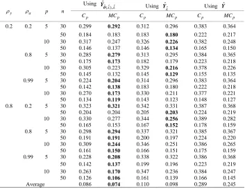
Each estimator optimized by using the MCp
crite-rion for , ˆθ, and q is more improve than that by using the Cp criterion for each estimator in almost all
situations. This indicates that the MCp criterion is a
better estimator of the MSE of each predicted value of
Y than the Cp criterion. The reasons for this are that
Table 1. MSE whenqis selected using each criterion for each method in each repetition(k6).
Using ˆ ˆ ˆ ( ),
ˆ
θ
Y Using Yˆˆ Using Yˆ y
a p n
p
C MCp C p MC p C p MC p
0.2 0.2 5 30 0.127 0.123 0.133 0.125 0.206 0.199 50 0.080 0.079 0.082 0.080 0.121 0.119 10 30 0.119 0.098 0.121 0.090 0.168 0.119
50 0.063 0.058 0.062 0.056 0.080 0.070
0.8 5 30 0.110 0.101 0.143 0.135 0.206 0.199 50 0.067 0.065 0.088 0.086 0.122 0.119 10 30 0.111 0.080 0.128 0.093 0.170 0.119 50 0.056 0.049 0.063 0.057 0.080 0.070 0.99 5 30 0.090 0.078 0.147 0.140 0.207 0.199 50 0.054 0.050 0.090 0.088 0.122 0.120 10 30 0.095 0.060 0.129 0.094 0.169 0.118 50 0.045 0.036 0.064 0.058 0.079 0.069 0.8 0.2 5 30 0.133 0.131 0.154 0.147 0.208 0.201 50 0.087 0.086 0.093 0.092 0.122 0.120 10 30 0.123 0.101 0.136 0.106 0.179 0.133 50 0.069 0.065 0.070 0.065 0.089 0.080 0.8 5 30 0.113 0.103 0.159 0.153 0.207 0.200 50 0.066 0.063 0.094 0.092 0.122 0.120 10 30 0.108 0.074 0.140 0.107 0.178 0.131 50 0.055 0.047 0.072 0.065 0.088 0.078 0.99 5 30 0.092 0.078 0.162 0.156 0.208 0.201 50 0.053 0.049 0.095 0.094 0.122 0.120 10 30 0.096 0.059 0.142 0.108 0.178 0.131 50 0.046 0.037 0.073 0.066 0.087 0.078 Average 0.086 0.074 0.110 0.098 0.147 0.130
Table 2. MSE whenqis selected using each criterion for each method in each repetition(k12).
Using ˆ ˆ ˆ ( ),
ˆ
θ
Y Using
ˆ
ˆ
Y Using Yˆ
y
a p n
p
C MC p C p MC p C p MC p
0.2 0.2 5 30 0.299 0.292 0.312 0.296 0.383 0.364
50 0.184 0.183 0.183 0.180 0.222 0.217
10 30 0.317 0.247 0.326 0.226 0.382 0.248
50 0.146 0.137 0.146 0.134 0.165 0.150
0.8 5 30 0.285 0.279 0.313 0.295 0.384 0.365
50 0.175 0.173 0.182 0.179 0.223 0.218
10 30 0.305 0.223 0.329 0.216 0.378 0.226
50 0.145 0.132 0.145 0.129 0.155 0.135
0.99 5 30 0.224 0.204 0.314 0.296 0.383 0.364
50 0.142 0.138 0.183 0.180 0.222 0.218
10 30 0.270 0.173 0.330 0.211 0.377 0.221
50 0.134 0.119 0.143 0.123 0.148 0.127
0.8 0.2 5 30 0.323 0.321 0.342 0.331 0.387 0.368
50 0.204 0.204 0.205 0.203 0.224 0.219
10 30 0.330 0.277 0.344 0.256 0.389 0.282
50 0.165 0.153 0.167 0.152 0.178 0.159
0.8 5 30 0.298 0.294 0.337 0.321 0.385 0.367
50 0.191 0.191 0.200 0.197 0.224 0.220
10 30 0.309 0.244 0.346 0.251 0.386 0.265
50 0.161 0.150 0.166 0.151 0.175 0.159
0.99 5 30 0.228 0.208 0.338 0.322 0.386 0.368
50 0.142 0.137 0.199 0.196 0.223 0.219
10 30 0.263 0.170 0.347 0.236 0.384 0.247
50 0.126 0.106 0.161 0.139 0.166 0.145
[image:9.595.122.475.437.710.2]