Electrical Load Forecasting Using Fuzzy System

(1)

ISSN Print: 2327-5219

DOI: 10.4236/jcc.2019.79003 Sep. 9, 2019 27 Journal of Computer and Communications

Electrical Load Forecasting Using Fuzzy System

Mahir Faysal

1

_{, Md. Jahirul Islam}

1

_{, Md. Mohiuddin Murad}

1

_{, Md. Imdadul Islam}

2

_{, M. Ruhul Amin}

3*

1_{Department of Electronics and Communications Engineering, East West University, Dhaka, Bangladesh} 2_{Department of Computer Science and Engineering, Jahangirnagar University, Savar, Bangladesh} 3_{Deparment of Mathematical and Physical Sciences, East West University, Dhaka, Bangladesh}

Abstract

To cope with the demand and supply of electrical load of an interconnected power system of a country, we need to forecast its demand in advance. In this paper, we use a fuzzy system to forecast electrical load on short-term basis. Here, we consider temperature, humidity, seasons of a year and time seg-ments of a day as the parameters, which govern the demand of electrical load. For each of the parameter, we use several membership functions (MFs) and then apply the Mamdani rule on MFs and the output is determined by using the centroid method. Finally, the surface plot reveals the real scenario of the load demand. The difference between actual load and the output of the fuzzy system is found as +1.65% to −13.76%. The concept of the paper can be ap-plied in interconnected power system of Bangladesh to reduce power loss, especially when generation is higher than the demand.

Keywords

Defuzzification, Fuzzy Inference, Centroid Method, Surface Plot, APE

1. Introduction

Electrical load forecasting is classified as short and long-term, where the long-term deals with adjustment of demand-supply for 10 - 50 years, whereas short-term makes the adjustment for a few months to 5 years. This paper con-siders short-term electrical load forecasting taking daily load of Bangladesh. This section provides some previous works relevant to short-term load forecasting. A study of the short-term electrical forecasting using fuzzy logic is done in [1] to minimize the difference between actual electrical load and the forecast load. The authors have used data from PSTCL 220 kV substation V.O.P Pakhowal, Lud-hiana, Punjab, India. Eight triangular membership functions (MFs) are used for How to cite this paper: Faysal, M., Islam,

Md.J., Murad, Md.M., Islam, Md.I. and Amin, M.R. (2019) Electrical Load Fore-casting Using Fuzzy System. Journal of Computer and Communications, 7, 27-37. https://doi.org/10.4236/jcc.2019.79003

Received: August 6, 2019 Accepted: September 6, 2019 Published: September 9, 2019

(2)

DOI: 10.4236/jcc.2019.79003 28 Journal of Computer and Communications input time, four triangular MFs for temperature and eight triangular MFs for output forecasted load; where input and output are linked using “if then” condi-tions. Finally, a comparison is made between actual load and fuzzy forecasted load graphically, where few points merge closely and few points deviate widely.

In [2], short-term load forecasting is done based on fuzzy logic, to find elec-trical load loss in the generation end. The authors prepare fuzzy rules based on historical data. A work is found about long term forecasting of power system in

[3], where the authors use Artificial Neural Network (ANN) and Adaptive Neu-ro-Fuzzy Interference System (ANFIS). Six parameters are used as input, which are temperature, humidity, wind speed, rainfall, data of previous load and data of actual load. A table is presented to compare the error between ANN and ANFIS, where the average error is 6.7% and 0.096% respectively.

Similar work is found in [4], based on ANN and Genetic where the data used for training and validation of the neural network is obtained from the Transmis-sion Company of Nigeria. First 21 days load and temperature data are used for training of neural network and the remaining day’s data is used for network va-lidation. Input variables used here are hour of the day, average temperature, day of the week and the output variable is forecasted load. After the evaluation, mean absolute percentage error (MAPE) is found about 4.705% for forecasting day. The authors of [5] established another related work using ANN taking data from Duhok ELC (Control region of Iraq) of 2009 and 2010. Back propagation algo-rithm of ANN is used to create a set of models where the AME is found differ-ent. The next day forecast is generated using the models, where the output is found almost close to the actual value. Another work on load forecasting using fuzzy logic tool is found in [6], which uses data from PSPCL 66 KV sub-station type-c grid. It is observed that in normal days, the load does not very much. However, in weekend or holiday, the load varies. After comparison, the error margin is found between +3.67% and −3.75%. A work on long-term electrical load forecasting using Multi-layer Perceptron Neural Network and K-Nearest Neighbor (K-NN) algorithm is presented in [7]. The data is collected from Global Energy Forecasting Competition 2018. The forecasted load is compared with the actual load for obtaining the MAPE, where MAPE of NN (MLP) is comparatively less than the K-NN method.

(3)

rain-DOI: 10.4236/jcc.2019.79003 29 Journal of Computer and Communications fall, wind speed, consumer price index and industrial index for year 1997-2007. The experimental result shows that multi regional area model can reduce error in each month and gives more accuracy than that of the whole country model. In

[10], a short-term load forecasting method is presented by utilizing neu-ron-wavelet method consisting of wavelet transform and soft computing tech-nique. The soft computing technique is featured by using the Generalized Neu-rons Network (GNN). Finally, a comparison is shown between GNN and mod-ified GNN, which shows that accuracy of forecasting increases in the combined model.

The prime objective of the paper is to reduce the difference between estimated power load and actual power load. At first, the actual data of energy consump-tion in twenty-four hours in a day for one fiscal year (2017-2018) is collected from Bangladesh Power Development Board’s (BPDB) website to determine the pattern of consumption and then we analyze them as MFs of our fuzzy system. The fuzzy toolbox of MATLAB is used to create rules considering four parame-ters: temperature, humidity, seasons and peak hour. The output is generated from the given input parameters. Finally, 3D surface plots are designed for the perception based on the output and the obtained results are compared with the results of the BPDB’s method.

The rest of the paper is organized as follows: Section 2 provides the basic theory of fuzzification and defuzzification along with the fuzzy model of elec-trical load forecasting, Section 3 provides the result based on the analysis of Sec-tion 2 and SecSec-tion 4 concludes the entire analysis.

2. Fuzzy Model of Load Forecasting

This section deals with a Fuzzy model, where the raw weather data is used as the input and the model will provide the electrical load. The first subsection gives the basic of centroid method in defuzzification and the second subsection gives fuzzy inference model of load forecasting.

2.1. Fuzzification and Defuzzification

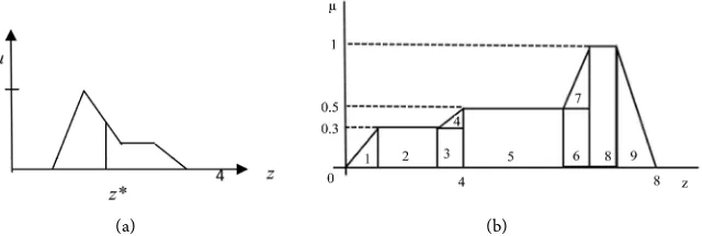
Fuzzy logic closely imitates the methodology in making human decision, as it deals with ambiguous and unsure information. In general, it is oversimplifica-tion of the real-world problems and based on degrees of truth rather than usual true/false or 1/0 like normal Boolean logic. Fuzzification is the process of forming a crisp set to a fuzzy set or a fuzzy set to fuzzier set. This operation trans-lates accurate crisp input values into linguistic variables. On the contrary, defuzzi-fication is the process of reducing a fuzzy set into a crisp set or to convert a fuzzy member into a crisp member. Among the different methods of defuzzification, centroid method is the most preferable and appealing method. This method is given by the expression like [11] [12],

* Ax

z

A

=

∑

(4)

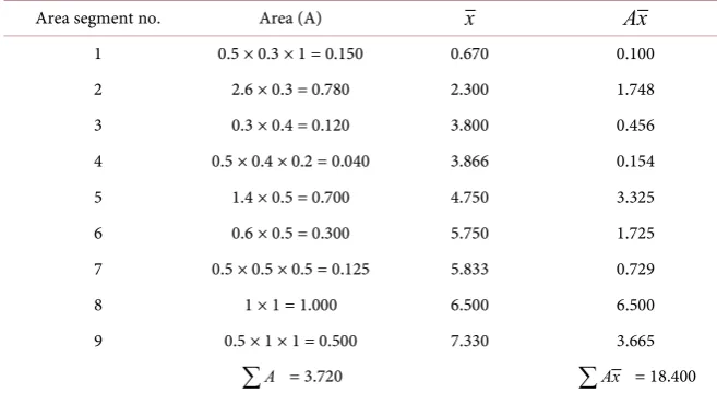
DOI: 10.4236/jcc.2019.79003 30 Journal of Computer and Communications This method is shown in Figure 1(a). Now, the expression for z* from Eq-uation (1) is applied to calculate the centroid of Figure 1(b), which is divided into segmented areas. Here, Table 1 shows the calculation of A and Ax for each segmented areas along with

_∑

A and

_∑

Ax.

Using Equation (1), we obtain

18.40

* 4.90

3.72

Ax z

A

=

∑

= =

∑

.

From this result, we can justify the defuzzification technique of centroid me-thod.

2.2. Load Forecasting Using Fuzzy Inference System

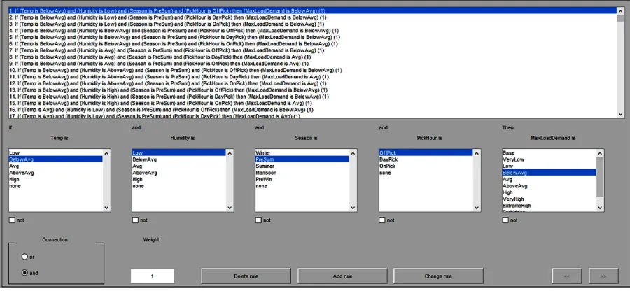
In this paper, the model for electrical load forecasting is implemented by utiliz-ing the centroid method of defuzzification in MATLAB. The collected data for each of the input parameters is processed by using “Mamdani” method and “if then” rule in fuzzy logic toolbox. Figure 2 represents the system in MATLAB. The first input is temperature and its five MFs and their ranges are low (0 - 15.5), below average (8 - 23), average (15.5 - 30.5), above average (23 - 38) and high (30.5 - 45) as shown in Figure 3. The second input is humidity, which is divided into five MFs with corresponding ranges that low (40 - 60), below aver-age (50 - 70), averaver-age (60 - 80), above averaver-age (70 - 90) and high (80 - 100) as shown in Figure 4. The third input is season and its five MFs with ranges (in days) are winter (11 - 70), pre-summer (46 - 132), summer (103 - 217), monsoon (188 - 305) and pre-winter (283 - 374) as shown in Figure 5. The fourth input is peak hour and its three MFs with ranges (in hours) are off peak (0 - 8), day peak (8 - 16) and on peak (16 - 23) as shown in Figure 6. We notice that for the fol-lowing parameters: temperature, humidity and season have two MFs as trape-zoidal in shape. All other MFs are in triangular. Only pick hour has three MFs, where all of them are trapezoidal. The output parameter is the maximum load demand, which has ten MFs with ranges (in MW) and these are: base (6000 - 7200), very low (6700 - 7700), low (7200 - 8200), below average (7700 - 8700), average (8200 - 9200), above average (8700 - 9700), high (9200 - 10,200), very high (9700 - 10,700), extreme high (10,200 - 11,200) and forbidden (11,700 - 12,000) as shown in Figure 7. The output parameter has two MFs as trapezoidal, which are base and forbidden. Except those, all other MFs are in triangular.

(a) (b)

[image:4.595.216.536.597.705.2]

(5)

[image:5.595.125.540.71.171.2]

DOI: 10.4236/jcc.2019.79003 31 Journal of Computer and Communications

[image:5.595.124.538.202.349.2]

Figure 2. Fuzzy logic load forecasting system in MATLAB.

Figure 3. Input parameter temperature.

Figure 4. Input parameter humidity.

[image:5.595.120.541.382.525.2] [image:5.595.125.538.559.705.2]

(6)

[image:6.595.122.540.72.220.2]

[image:6.595.120.543.252.400.2]

Figure 6. Input parameter peak hour.

Figure 7. Output parameter maximum load demand.

Table 1. Weighted sum of areas.

Area segment no. Area (A) x Ax

1 0.5 × 0.3 × 1 = 0.150 0.670 0.100

2 2.6 × 0.3 = 0.780 2.300 1.748

3 0.3 × 0.4 = 0.120 3.800 0.456

4 0.5 × 0.4 × 0.2 = 0.040 3.866 0.154

5 1.4 × 0.5 = 0.700 4.750 3.325

6 0.6 × 0.5 = 0.300 5.750 1.725

7 0.5 × 0.5 × 0.5 = 0.125 5.833 0.729

8 1 × 1 = 1.000 6.500 6.500

9 0.5 × 1 × 1 = 0.500 7.330 3.665

A

∑

= 3.720

∑

Ax = 18.400

[image:6.595.208.537.452.632.2]

(7)

DOI: 10.4236/jcc.2019.79003 33 Journal of Computer and Communications applied in the input box of the rule viewer. In surface plot viewer, as shown in

Figure 10, surface plot of load forecasting using fuzzy inference system is pre-sented graphically by utilizing the given rules.

3. Results and Discussion

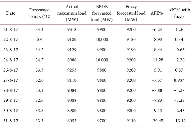
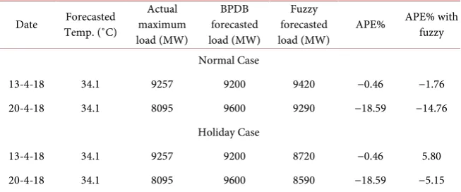
[image:7.595.72.522.500.708.2]

First, a comparison of BPDB and Fuzzy forecasting is shown in Tables 2-4 for three seasons: monsoon, winter and summer respectively. Here, we only show the results taking 10 days from each month to make the data concise for the pa-per. After analyzing our results, we can see significant improvements in average percentage of error when using our forecasting method compared to the method used by BPDB. Therefore, it is quite safe to assume that our fuzzy inference sys-tem is better structured and cost efficient than the BPDB’s syssys-tem. However, with our methodology, load forecasting of holidays shows erratic results. The BPDB’s method shows similar behavior in terms of holiday load forecasting. For this reason, we subtract seven hundred MW from the ranges of the output membership function’s parameters and re-create a new fuzzy inference system with all other input parameters and their MF’s ranges unchanged, which is only applicable for holidays. A comparison of normal and holiday load forecasting method is shown in Tables 5-7 for three seasons: monsoon, winter and summer. A little improvement is achieved when applying holiday load forecasting method for the holidays compared to normal load forecasting method. Still, we are not able to achieve quite significant improvements, as the usage of load during holi-days is very much unpredictable. It does not follow any usual patterns (abrupt variation of data), which is seen in case of normal days. In this case, one possible solution is to smooth the abrupt variation of load of holidays using multiple li-near regressions (MLR) then smooth data can be applied in FIS model to im-prove the accuracy. This will be the extension of our work in future.

(8)

[image:8.595.60.541.64.305.2]

Figure 9. Load forecasting rules in rule viewer.

Figure 10. Surface plot in 3D.

Table 2. August’ 17 comparison of forecasting data.

Date _{Temp. (˚C)}Forecasted maximum load Actual (MW)

BPDB forecasted load (MW)

Fuzzy forecasted load

(MW) APE% APE% with fuzzy

21-8-17 34.4 9318 9900 9200 −6.24 1.26

22-8-17 33 9180 10,000 9130 −8.93 0.54

23-8-17 34.2 9129 9900 9190 −8.44 −0.66

24-8-17 34.7 8986 10,000 9200 −11.28 −2.38

26-8-17 33.3 9253 9800 9200 −5.91 0.57

27-8-17 32.6 9110 9800 9200 −7.57 0.987

28-8-17 33.1 9084 9800 9200 −7.88 −1.27

29-8-17 32.6 9088 9800 9200 −7.83 −1.23

30-8-17 33.8 8980 9800 9200 −9.13 −2.45

[image:8.595.212.539.509.734.2]

(9)

[image:9.595.210.540.88.243.2]

Table 3. February’ 18 comparison of forecasting data.

Date _{Temp. (˚C)}Forecasted maximum Actual load (MW) BPDB forecasted load (MW) Fuzzy forecasted

load (MW) APE%

APE% with fuzzy

1-2-18 25.8 8162 8350 8300 −2.30 −1.69

3-2-18 28 8109 8000 8200 1.34 −1.12

4-2-18 29.7 8139 8350 8200 −2.59 −0.74

5-2-18 29.3 8247 8350 8200 −1.24 0.56

6-2-18 28.7 7976 8400 8200 −5.31 −2.80

7-2-18 28.4 8258 8400 8360 −1.71 −1.25

8-2-18 28.3 8115 8400 8290 −3.51 −2.15

[image:9.595.209.539.273.444.2]

10-2-18 27.5 8144 8350 8330 −2.52 −2.29

Table 4. April’ 18 comparison of forecasting data.

load (MW) APE%

APE% with fuzzy

10-4-18 32.2 9355 9900 9200 −5.82 1.65

11-4-18 33.1 8943 10,000 9430 −11.81 −5.44

12-4-18 33.8 8917 9650 9560 −8.22 −7.21

14-4-18 33.4 7665 9300 8720 −21.33 −13.76

15-4-18 37.5 9961 9800 9860 1.61 1.01

16-4-18 36.4 9702 10,100 9560 −4.10 1.46

17-4-18 37 8464 10,100 9050 −19.32 −6.92

18-4-18 37.1 9758 10,000 9650 −2.54 1.10

19-4-18 32.4 9425 10,000 9300 −6.10 1.32

Table 5. August’ 17 forecasted load error comparison using normal and holiday case.

load (MW) APE%

APE% with fuzzy

Normal Case

25-8-17 34.7 8933 9800 9200 −9.70 −2.98

Holiday Case

25-8-17 34.7 8933 9800 8500 −9.70 4.84

Table 6. February’ 18 forecasted load error comparison using normal and holiday case.

Date _{Temp. (˚C)}Forecasted maximum load Actual (MW) BPDB forecasted load (MW) Fuzzy forecasted

load (MW) APE%

APE% with fuzzy Normal Case

2-2-18 26.2 7262 7500 8200 −3.27 −12.91

9-2-18 30.4 7449 7500 8210 −0.68 −10.21

Holiday Case

2-2-18 26.2 7262 7500 7500 −3.27 −3.27

[image:9.595.209.539.475.567.2] [image:9.595.211.539.599.730.2]

(10)

[image:10.595.212.539.89.225.2]

Table 7. April’ 18 forecasted load error comparison using normal and holiday case.

Date _{Temp. (˚C)}Forecasted maximum Actual load (MW)

BPDB forecasted load (MW)

Fuzzy forecasted

load (MW) APE%

APE% with fuzzy

Normal Case

13-4-18 34.1 9257 9200 9420 −0.46 −1.76

20-4-18 34.1 8095 9600 9290 −18.59 −14.76

Holiday Case

13-4-18 34.1 9257 9200 8720 −0.46 5.80

20-4-18 34.1 8095 9600 8590 −18.59 −5.15

4. Conclusion

In this paper, we have applied microscopic approach and developed fuzzy infe-rence model applicable in short term and long term forecasting of real life prob-lems. Here, we have considered the concept of electrical load forecasting of Ban-gladesh, taking the practical data of BPDB. We have correlated the demand of electrical load with weather parameters and have found high accuracy in winter season. In future, we have the scope to apply MLR, back propagation algorithm of ANN, Long Short Term Memory (LSTM) of machine learning and convolu-tional neural network (CNN) of deep learning to relate the weather parameters with the actual electrical load for comparison.

Conflicts of Interest

The authors declare no conflicts of interest regarding the publication of this pa-per.

References

[1] Kaur, J. and Brar, Y.S. (2014) Short Term Electrical Forecasting Using Fuzzy Logic of 220kV Transmission Line. International Journal of Engineering Research & Technology, 3, 336-343.

[2] Ali, A.T., Tayeb, E.B.M. and Shamseldin, Z.M. (2016) Short Term Electrical Load Forecasting Using Fuzzy Logic. International Journal of Advancement in Engineer-ing Technology, Management and Applied Science, 3, 131-138.

[3] Ammar, N., Sulaiman, M. and Nor, A.F.M. (2018) Long Term Load Forecasting of Power Systems Using Artificial Neural Network and ANFIS. ARPN Journal of En-gineering and Applied Sciences, 13, 828-834.

[4] Olagoke, M.D., Ayeni, A.A. and Hambali, M.A. (2016) Short Term Electric Load Forecasting Using Neural Network and Genetic Algorithm. International Journal of Applied Information Systems, 10, 22-28. https://doi.org/10.5120/ijais2016451490

[5] Melhum, A.I., Omar, L. and Mahmood, S.A. (2013) Short Term Load Forecasting Using Artificial Neural Network. International Journal of Soft Computing and En-gineering, 3, 56-58.

[6] Singla, M.K. and Hans, S. (2018) Load Forecasting Using Fuzzy Logic Tool Box.

(11)

[7] Patel, M.R., Patel, R.V., Dabhi, D. and Patel, J.S. (2019) Long Term Electrical Load Forecasting Considering Temperature Effect Using Multi-Layer Perceptron Neural Network and k-Nearest Neighbor Algorithms. International Journal of Research in Electronics and Computer Engineering, 7, 823-827.

[8] Ali, D., Yohanna, M., Puwu, M.I. and Garkida, B.M. (2016) Long-Term Load Fore-cast Modelling Using a Fuzzy Logic Approach. Pacific Science Review A: Natural Science and Engineering, 18, 123-127. https://doi.org/10.1016/j.psra.2016.09.011

[9] Bunnoon, P., Chalermyanont, K. and Limsakul, C. (2010) The Comparison of Mid Term Load Forecasting between Multi-Regional and Whole Country Area Using Artificial Neural Network. International Journal of Computer and Electrical Engi-neering, 2, 334-338. https://doi.org/10.7763/IJCEE.2010.V2.157

[10] Chaturvedi, D.K., Premdayal, S.A. and Chandiok, A. (2010) Short-Term Load Fo-recasting Using Soft Computing Techniques. International Journal of Communica-tions, Network and System Sciences, 3, 273-279.

https://doi.org/10.4236/ijcns.2010.33035

[11] Saneifard, R. and Saneifard, R. (2011) A Method for Defuzzification Based on Cen-troid Point. Turkish Journal of Fuzzy Systems, 2, 36-44.