NUMERICAL ANALYSIS OF THE TUBE BANK PRESSURE DROP OF A SHELL AND TUBE
HEAT EXCHANGER USING FLAT FACE HEADER
*1
Kartik Ajugia,
2Aksheshkumar A. Shah,
1Assistant Professor, Mechanical Department,
2Dwarkadas J. Sanghvi College of Engineering, University of
ARTICLE INFO ABSTRACT
Pressure drop is the main parameters describing the efficiency and acceptance of a particular shell and tube heat exchanger in any application.
the viz. Higher the pressure drop lower is the heat transfer and hence the required pumping power is high and correspondingly higher is the expense. The pressure drop on the tube side can be trichotomized as pressure drop due to
in the outlet nozzle. This report provides an insight into the research done on the analysis of the pressure drop in the tubes of a shell and tube heat exchanger. Although a remarkable contri
been done through analytical relations governing the pressure drop and the numerical analysis of the pressure drop on the shell side of a shell and tube heat exchanger, cogent contribution can be made numerically on the tube side. The approach p
(pressure drop) in the tubes using the TEMA BEM viz. a Flat Head Single Pass SHTX numerically viz. the use of computation for the mentioned research. Hence to achieve the task numerically the use of ANSYS1
zones have been identified viz. (1) High pressure drop zone (2) Low pressure drop zone across the tube banks. It was observed that nearly fifty percent of the tubes li
drop has been computed numerically at a specific inlet velocity and then correlated at different inlet velocities for a parametric study.
Copyright © 2018, Kartik Ajugia et al. This is an open distribution, and reproduction in any medium, provided
INTRODUCTION
A heat exchanger is an instrument used to transfer heat from one medium to another by segregating them to prevent mixing or allowing them to mix and transfer the heat. One such example of an exchanger which prevents the mixing of the mediums is a shell and tube heat exchanger. There are multiple types of shell and tube heat exchangers based on their geometrical parameters. However for the present analysis, a TEMA BEM (TEMA, 1999), has been used. The various tube side of a SHTX consists of the inlet nozzle,
bank, outlet header and the outlet nozzle. The pressure drop plays acritical role in the overall efficiency of a SHTX. The total tube-side pressure drop ΔPT for a single pass constitutes of the pressure drop in the straight tubes (ΔPTT),
in the tube entrances, exits and reversals (ΔPTE), and pressure drop in nozzles (ΔPTN) (Serth, 2007).
*Corresponding author: Kartik Ajugia
Assistant Professor, Mechanical Department, Dwarkadas J. Sanghvi College of Engineering, University of Mumbai
ISSN: 0975-833X
Vol. 10, Issue, 09,
Article History:
Received 17th June, 2018 Received in revised form 22nd July, 2018
Accepted 06th August, 2018
Published online 30th September, 2018
Citation: Kartik Ajugia, Aksheshkumar A. Shah, Rohit A. Rawool,
pressure drop of a Shell and tube heat exchanger using flat face header
Key Words:
Pressure drop;
Shell and tube heat Exchangers; Tube Side; numerically.
RESEARCH ARTICLE
NUMERICAL ANALYSIS OF THE TUBE BANK PRESSURE DROP OF A SHELL AND TUBE
HEAT EXCHANGER USING FLAT FACE HEADER
Aksheshkumar A. Shah,
2Rohit A. Rawool,
2Siddharth S. Saini and
2
Tejas P. Shah
Assistant Professor, Mechanical Department, Dwarkadas J. Sanghvi College of Engineering, University of Mumbai Dwarkadas J. Sanghvi College of Engineering, University of Mumbai
ABSTRACT
Pressure drop is the main parameters describing the efficiency and acceptance of a particular shell and tube heat exchanger in any application. Pressure drop across the tube side i
the viz. Higher the pressure drop lower is the heat transfer and hence the required pumping power is high and correspondingly higher is the expense. The pressure drop on the tube side can be trichotomized as pressure drop due to Inlet nozzle, pressure drop in the tube bank, and pressure drop in the outlet nozzle. This report provides an insight into the research done on the analysis of the pressure drop in the tubes of a shell and tube heat exchanger. Although a remarkable contri
been done through analytical relations governing the pressure drop and the numerical analysis of the pressure drop on the shell side of a shell and tube heat exchanger, cogent contribution can be made numerically on the tube side. The approach provided enables us to study detailed flow behavior (pressure drop) in the tubes using the TEMA BEM viz. a Flat Head Single Pass SHTX numerically viz. the use of computation for the mentioned research. Hence to achieve the task numerically the use of ANSYS16.0has been made assuming that the flow is steady and isothermal. Two different pressure zones have been identified viz. (1) High pressure drop zone (2) Low pressure drop zone across the tube banks. It was observed that nearly fifty percent of the tubes li
drop has been computed numerically at a specific inlet velocity and then correlated at different inlet velocities for a parametric study.
access article distributed under the Creative Commons Attribution the original work is properly cited.
A heat exchanger is an instrument used to transfer heat from one medium to another by segregating them to prevent mixing or allowing them to mix and transfer the heat. One such example of an exchanger which prevents the mixing of the tube heat exchanger. There are multiple types of shell and tube heat exchangers based on their geometrical parameters. However for the present analysis, a has been used. The various tube side of a SHTX consists of the inlet nozzle, inlet header, tube bank, outlet header and the outlet nozzle. The pressure drop plays acritical role in the overall efficiency of a SHTX. The side pressure drop ΔPT for a single pass constitutes of the pressure drop in the straight tubes (ΔPTT), pressure drop in the tube entrances, exits and reversals (ΔPTE), and pressure
Assistant Professor, Mechanical Department, Dwarkadas J. Sanghvi
The uniform distribution of flow in tube bundle of shell and tube heat exchangers is an assumption in conventional heat exchanger design as claimed by Bejan and Kraus
2003). Traub (Traub, 1990), found that increased turbulence levels lead to an enhancement in the heat transfer for tube banks with a few rows of plain circular tubes at small pitch to diameter ratios. Contrarily, the aim of the passive techniques is to alter the flow by changing the
Achenbach (Achenbach, 1991).
bank pressure drop of a shell and tube heat exchanger Ajugia, 2015), found that rough surfaces on the tubes of in arrangements in cross-flow have the poten
pressure drop while simultaneously improving heat transfer, at least within a particular range of Reynolds numbers, which is determined by the roughness parameter.
Physical Modelling
In order to design the geometry of an actual tube arrangement, numerous manufacturing industries had been visited of which CANAAN Engineering Works provided the
International Journal of Current Research
Vol. 10, Issue, 09, pp.73693-73697, September, 2018
DOI: https://doi.org/10.24941/ijcr.32469.09.2018
ksheshkumar A. Shah, Rohit A. Rawool, Siddharth S. Saini and Tejas P. Shah. 2018. “Numerical analysis of The Tube Bank
pressure drop of a Shell and tube heat exchanger using flat face header”, International Journal of Current Research, 10, (
NUMERICAL ANALYSIS OF THE TUBE BANK PRESSURE DROP OF A SHELL AND TUBE
HEAT EXCHANGER USING FLAT FACE HEADER
Siddharth S. Saini and
Dwarkadas J. Sanghvi College of Engineering, University of Mumbai Mumbai
Pressure drop is the main parameters describing the efficiency and acceptance of a particular shell and Pressure drop across the tube side is inversely proportional to the viz. Higher the pressure drop lower is the heat transfer and hence the required pumping power is high and correspondingly higher is the expense. The pressure drop on the tube side can be Inlet nozzle, pressure drop in the tube bank, and pressure drop in the outlet nozzle. This report provides an insight into the research done on the analysis of the pressure drop in the tubes of a shell and tube heat exchanger. Although a remarkable contribution has been done through analytical relations governing the pressure drop and the numerical analysis of the pressure drop on the shell side of a shell and tube heat exchanger, cogent contribution can be made rovided enables us to study detailed flow behavior (pressure drop) in the tubes using the TEMA BEM viz. a Flat Head Single Pass SHTX numerically viz. the use of computation for the mentioned research. Hence to achieve the task numerically the use 6.0has been made assuming that the flow is steady and isothermal. Two different pressure zones have been identified viz. (1) High pressure drop zone (2) Low pressure drop zone across the tube banks. It was observed that nearly fifty percent of the tubes lie under each category. The pressure drop has been computed numerically at a specific inlet velocity and then correlated at different inlet
License, which permits unrestricted use,
The uniform distribution of flow in tube bundle of shell and tube heat exchangers is an assumption in conventional heat exchanger design as claimed by Bejan and Kraus (Bejan, found that increased turbulence levels lead to an enhancement in the heat transfer for tube banks with a few rows of plain circular tubes at small pitch to diameter ratios. Contrarily, the aim of the passive techniques is to alter the flow by changing the geometry of the arrangement. , 1991). Numericalanalysis of the tube bank pressure drop of a shell and tube heat exchanger (Kartk found that rough surfaces on the tubes of in-line flow have the potential to decrease the pressure drop while simultaneously improving heat transfer, at least within a particular range of Reynolds numbers, which is determined by the roughness parameter.
In order to design the geometry of an actual tube side arrangement, numerous manufacturing industries had been visited of which CANAAN Engineering Works provided the
OF CURRENT RESEARCH
drawing of an actual manufactured shell and tube heat exchanger which was to be used in an industry located at Hazira , Surat.
[image:2.595.307.563.49.184.2]The geometrical parameters for the heat exchanger are shown in Table - 1
Table 1. Geometrical Parameters Ref.
Sr No Geometrical Parts
1 Inlet/Outlet Header
2 Shell or Header I.D
3 No of Tubes
4 Tube O.D
5 Tube Thickness
6 Inlet and Outlet Nozzle I.D
7 Nozzle Lengths
8 Tube Pitch
9 Tube Layout
10 Tube Length
11 Fluid circulated
12 Fluid Density
13 Fluid Viscosity
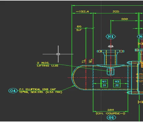
[image:2.595.44.282.158.297.2]The pictures of the AutoCAD drawings used are as shown Ref.[6]:
Fig. 1. Geometrical specification Ref.[6]
Fig. 2. Geometrical Specification
Based on the above dimensional specification and the two dimensional drawing the three dimensional
was designed using ANSYS ICEM 16.0 version.
drawing of an actual manufactured shell and tube heat exchanger which was to be used in an industry located at
rical parameters for the heat exchanger are shown
Ref. [6]
Specifications Flat Ends 2: 1 304.8 mm 77 19.05 mm 1.65 mm 66.64 mm 212 mm 25.4 mm Triangular (600) 1518 mm Water
998.2 kg/m3
0.001003 kgm/s
The pictures of the AutoCAD drawings used are as shown
Geometrical specification Ref.[6]
Geometrical Specification
[image:2.595.37.289.343.559.2]Based on the above dimensional specification and the two dimensional drawing the three dimensional physical models was designed using ANSYS ICEM 16.0 version.
Fig. 3. 3 –D model of SHTX
The figure numbers 1, 2, 3 represent the geometrical dimension and the actual model for analyses. However the thickness was not taken into consideration as the rese
carried out for pressure drop is irrespective of the thickness of the model.
Meshing
Both the Flat end and the flat face headers were meshed
in ICEM.
The global mesh setup, surface mesh setup and the
curve mesh setup were done initially to
mesh. The method used for volume mesh setup was tetra/mixed robust octree.
Post the creation of Surface mesh, it was further meshed
in 3-D using prism mesh with two layers created near the curve surfaces to capture the boundary layer flow precisely.
A number of smoothening iterations were done in order
to improve quality of the mesh. The quality of the mesh thus obtained was pretty acceptable.
The fig – 4 is of the meshed geometry:
Fig. 4. Meshed Geometry
The mesh thus obtained consisted of 2519375 cells or 489085 nodes. The mesh obtained was of high qualitywith a minimum value of 0.25. Nonetheless, there were a very few nodes which had a slightly lesser quality than that indicted which was overlooked as they were infinitesimally
meshed file was then imported in ANSYS FLUENT for further analysis.
Solver Setup
The governing equations used by the solver shall include the Continuity and the Navier Stokes Equation viz. the Momentum Equations in three dimensions.
D model of SHTX
The figure numbers 1, 2, 3 represent the geometrical dimension and the actual model for analyses. However the thickness was not taken into consideration as the research to be carried out for pressure drop is irrespective of the thickness of
Both the Flat end and the flat face headers were meshed
The global mesh setup, surface mesh setup and the curve mesh setup were done initially to create surface mesh. The method used for volume mesh setup was tetra/mixed robust octree.
Post the creation of Surface mesh, it was further meshed D using prism mesh with two layers created near the curve surfaces to capture the boundary layer flow
A number of smoothening iterations were done in order to improve quality of the mesh. The quality of the mesh thus obtained was pretty acceptable.
4 is of the meshed geometry:
Meshed Geometry
consisted of 2519375 cells or 489085 nodes. The mesh obtained was of high qualitywith a minimum value of 0.25. Nonetheless, there were a very few nodes which had a slightly lesser quality than that indicted which was overlooked as they were infinitesimally small in number. The meshed file was then imported in ANSYS FLUENT for further
[image:2.595.308.562.493.608.2] [image:2.595.37.295.590.722.2]The boundary conditions used for the solver setup are as shown in table no – 2.
Table 2. Boundary conditions for various parts Ref. [6]
Sr No Name of the Zone Boundary
Condition
Boundary Characteristics
1 Inlets Velocity Inlet 3.31 (m/s)
2 Outlets Pressure
Outlets
0 Gauge Pressure
3 Inlet Wall Wall No Slip, Surface
Roughness 0.5,
Stationary
4 Outlet Wall
5 Tube walls
6 Header Walls
The solution method used was the “SIMPLE” Algorithm and the spatial discretization was based on Second Order Upwind Scheme. The turbulence model used was the standard k-ε model. The solution was run for 1000 iterations.
RESULTS AND ANALYSIS
Analytical Pressure drop across the tubes. The input velocity to the nozzle was chosen as 3.31 m/s. The tube side pressure drop constitutes of the pressure drop due to friction losses inside the tubes plus the pressure losses due to sudden expansion and contractions which is accounted by four velocity heads per pass [6]. Therefore the total pressure drop for the tube side fluid flow is given by
ΔPt = 4 * f * L* Np * ρ * U2m / (2 * di )
ΔPr = 4 * Np * ρ * U
2
m / 2
ΔP total = (4 * f * L * Np / di + 4 * Np ) ρ * U2m / 2
Where
ΔPtand ΔPrare the pressure losses due to friction and sudden
expansions and contraction respectively L – Length of the tubes (1.518 m)
Np - No of passes (One Pass)
di - Inner diameter of the tubes (0.01575 m)
Um – Mean velocity of Fluid in the tubes
f – friction factor, ρ – Density of the fluid (998.2 kg/m3)
The friction factor f is given by Moody’s chart for turbulent
flow through uniform circular pipes [7] viz. f = 0.079Re-0.25
where Re is the Reynold no for the fluid. As per the given conditions the pressure drop for a single pass tube side was found to be analytically = 2038 Pascal. Another correlation for the tube side pressure drop was given by R. W Serth[2] who suggests that the total tube-side pressure drop ΔPT for a single pass comprises the pressure drop in the straight tubes (ΔPTT), pressure drop in the tube entrances, exits and reversals (ΔPTE).
ΔPT = (ΔPTT) + (ΔPTE)
Where
ΔPTT = KPT1 * NP * L * uT(2 + mf )
KPT1 = 2 * FC ((ρ * d1 / µ) ^ mf ) * ρ/ d1
FC = 0.0791 , mf = - 0.25 for Re ≥ 3000
ΔPTE = KPT2 * u2T
KPT2 = 4 * αR * ρ
αR = 2 Np – 1.5
uT - mean velocity of the fluid through the tubes which is the
same as that obtained above. It was observed that using the above correlation also the pressure drop was found to be 2038 Pascal.
Numerical Pressure drop across the tube bundle
[image:3.595.306.565.263.401.2]The meshed file was imported and after doing so the Solver setup mentioned earlier, the 1000 iteration were run. The solution converged in less than 300 iteration. Figure 5 represents the tube array in the geometric mode.
Fig. 5. Tube bundle Array Ref. [6]
[image:3.595.306.559.663.782.2]The origin for the geometry was at the tip of the Flat wall at the inlet header. The distance between the origin and the start of the tube bundle is 392 mm. Inorder to find the numerical pressure drop a number of Z- Coordinates viz. vertical sections in the X – Y plane passing through the tube arrays through the center were created with the center one being the Z – 0. Moving along the positive Z axis as shown in fig 5 each vertical tube bundle is separated from each other by half a pitch viz. 25.4/2 = 12.7 mm. Therefore a total of 19 such Z Coordinates were created inorder to capture the 77 tubes of which 9 were along the positive Z – axis and 9 along the negative plus the center one. Also an X coordinate at a distance of 5 mm away from the tube start was created. Thus combustion of the various Z Coordinates and the single X Coordinate the pressure at the inlet of each and every tube was found out. A gap of 4 mm was left between the tube start and the X Coordinate inorder to capture the pressure changes due to entrance effect of fluid inside the tube from the header. The fig 6 shows the Z – 0 coordinate of contours of total pressure which captures the centermost array of tubes 5 in numbers.
The fig 7 shows the X – Coordinate.
[image:4.595.39.291.74.199.2]Pressure contour at X=378
Fig. 7. X-Coordinate 4 mm away from tube bundle
Grid Sensitivity Test
[image:4.595.308.561.365.547.2]Before running the simulation, an optimized mesh needs to be found out in terms of the accuracy of the results and the lesser number of nodes inorder to reduce the computation cost. geometrical model was meshed for three different dimension inorder to obtain a coarse, medium and a fine mesh. The numbers of cells thus obtained are mentioned in the table no 3
Table 3. Grid Independence Test Ref. [6]
Sr No Mesh Type Number of
Cells
Average pressure Drop Across Tube Side
1 Coarse Mesh 1986668 1918
2 Medium Mesh 2519375 1943
3 Fine Mesh 3709885 1912
Fig. 8. Grid Independence Test Ref. [6]
The fig no - 8 illustrates that the average pressure drop increases reaches optimum and then starts decreasing as the fineness goes on increasing. Thus the optimum mesh used for further simulations was the medium. The highest accuracy obtained from the mesh was with a -4.6 % deviation from the theoretical results. The medium mesh selected also helps to reduce the computation cost compared to that of the fine mesh.
Inferences
A two set of pressure values were obtained at the inlet
of the tubes.
The tubes with green color at the start of the tubes in the
fig no 6 and 7 indicates a pressure value of 10506 Pa while the yellow color indicates 11285 Pa.
Coordinate 4 mm away from tube bundle
Before running the simulation, an optimized mesh needs to be found out in terms of the accuracy of the results and the lesser ce the computation cost. The geometrical model was meshed for three different dimension inorder to obtain a coarse, medium and a fine mesh. The numbers of cells thus obtained are mentioned in the table no –
Grid Independence Test Ref. [6]
Average pressure Drop Across Tube Side
Fig. 8. Grid Independence Test Ref. [6]
8 illustrates that the average pressure drop first increases reaches optimum and then starts decreasing as the fineness goes on increasing. Thus the optimum mesh used for The highest accuracy 4.6 % deviation from the esults. The medium mesh selected also helps to reduce the computation cost compared to that of the fine mesh.
A two set of pressure values were obtained at the inlet
The tubes with green color at the start of the tubes in the no 6 and 7 indicates a pressure value of 10506 Pa while the yellow color indicates 11285 Pa.
All the 77 tubes were observed at the inlet side with the
help of Z and X Coordinates to get the inlet pressures of the respective tubes.
38 tubes were having a pressure inlet of 11285 Pa while
39 tubes were having a pressure inlet of 10506 Pa.
It can be observed from fig no 6 as well as all the Z
Coordinates that at the outlet all the tubes had a uniform pressure viz. there is not much variation.
The outlet pressure was observed as 8947Pa.
Therefore the average pressure drop can be calculated
as [(39 * 10506 + 38 * 11285)
From the above calculation the average pressure drop
was found to be 1943.5 Pa while the theoretical average pressure drop is 2038 Pa.
The difference between the theoretical and the
numerical analysis is less than 10% which is within the acceptable range, hence the results are validated.
Parametric Study
The simulations were run for different input velocities of 2m/s, 5m/s and 7 m/s at the inlet nozzle and a relationship between the theoretical and numerical pressure drops were observed. Table no – 5 indicates the parametric study.
Table 5. Parametric study with different velocities
Input Velocities 3.31m/s
ΔPtheor (Pa) 2030
ΔPnum(Pa) 2136
% Difference 5.2
Chart 1. Parametric study of various Velocities
Purple colored line in chart 1 indicates pressure drop
line for theoretical values at various velocities while the pink one is for numerical.
As the inlet velocity goes on increasing the %
difference goes on decreasing as indicated in table no 5.
Conclusions
The numerical study gave an idea of the pressure drop
taking across each tube whereas the theoretical expressions just provided us with the average pressure drops across the tube banks.
Numerical analysis helped us to identify the two
pressure zones at the inlet header viz. a low pressure drop zone approximately at the upper half while a high pressure drop at the lower hal
The numerical results were validated against the
theoretical results.
All the 77 tubes were observed at the inlet side with the help of Z and X Coordinates to get the inlet pressures
pressure inlet of 11285 Pa while 39 tubes were having a pressure inlet of 10506 Pa. It can be observed from fig no 6 as well as all the Z Coordinates that at the outlet all the tubes had a uniform pressure viz. there is not much variation.
ure was observed as 8947Pa.
Therefore the average pressure drop can be calculated as [(39 * 10506 + 38 * 11285) – 77* 8947)] / 77. From the above calculation the average pressure drop was found to be 1943.5 Pa while the theoretical average
s 2038 Pa.
The difference between the theoretical and the numerical analysis is less than 10% which is within the acceptable range, hence the results are validated.
The simulations were run for different input velocities of 2m/s, d 7 m/s at the inlet nozzle and a relationship between the theoretical and numerical pressure drops were observed.
5 indicates the parametric study.
Parametric study with different velocities
3.31m/s 5m/s 7m/s
2030 4439 8422
2136 4683 7715
5.38 -6
Parametric study of various Velocities
Purple colored line in chart 1 indicates pressure drop line for theoretical values at various velocities while the
is for numerical.
As the inlet velocity goes on increasing the % difference goes on decreasing as indicated in table no 5.
The numerical study gave an idea of the pressure drop taking across each tube whereas the theoretical provided us with the average pressure drops across the tube banks.
Numerical analysis helped us to identify the two pressure zones at the inlet header viz. a low pressure drop zone approximately at the upper half while a high pressure drop at the lower half.
[image:4.595.36.282.368.593.2] This study can further be used for other research work related to the tube side.
Acknowledgement
Wewould like to thank Professor Kartik Ajugia for his invaluable guidance and efforts in accomplishing this task.
REFERENCES
Bejan, A., Kraus, A.D., 2003. Heat Transfer Handbook. John Wiley & Sons, New Jersey.
D. Traub, Turbulent heat transfer and pressure drop in plain tube bundles, Chem. Eng. Process. 28 (1990) 173–181. E. Achenbach, Heat transfer from smooth and rough in-line
tube banks at high Reynolds numbers, Int. J. Heat Mass
Transfer 34 (1) (1991) 199–207.
Harrison (Editor), Tubular Exchanger Manufacturers
Association, Inc., 8th Edition, USA
KartkAjugia, Kunal Bhavsar, Numerical analysis of the tube bank pressuredrop of a shell and tube heat exchanger, ICMPIAE 2015.
Kern, D.Q, Process Heat Transfer, McGraw-Hill, New York, 1950.
Moody, L.F., Friction factor for pipe flow, Trans. ASME, 66,671, 1994.
R.W. Serth, Process Heat Transfer: Principles and Applications, Burlington Academic Press, 2007.
TEMA, 1999. Standards of the Tubular Exchanger Manufacturers Association, J.
![Fig. 5. Tube bundle Array Ref. [6]](https://thumb-us.123doks.com/thumbv2/123dok_us/9081487.404864/3.595.306.565.263.401/fig-tube-bundle-array-ref.webp)
![Table 3. Grid Independence Test Ref. [6]Grid Independence Test Ref. [6]](https://thumb-us.123doks.com/thumbv2/123dok_us/9081487.404864/4.595.36.282.368.593/table-grid-independence-test-ref-grid-independence-test.webp)
