Spontaneous reconnection at a separator current layer:
2. Nature of the waves and flows
J. E. H. Stevenson1and C. E. Parnell1
1School of Mathematics and Statistics, Mathematical Institute, St Andrews, Scotland
Abstract
Sudden destabilizations of the magnetic field, such as those caused by spontaneous reconnection, will produce waves and/or flows. Here we investigate the nature of the plasma motions resulting from spontaneous reconnection at a 3-D separator. In order to clearly see these perturbations, we start from a magnetohydrostatic equilibrium containing two oppositely signed null points joined by a generic separator along which lies a twisted current layer. The nature of the magnetic reconnection initiated in this equilibrium as a result of an anomalous diffusivity is discussed in detail in Stevenson and Parnell (2015). The resulting sudden loss of force balance inevitably generates waves that propagate away from the diffusion region carrying the dissipated current. In their wake a twisting stagnation flow, in planes perpendicular to the separator, feeds flux back into the original diffusion site (the separator) in order to try to regain equilibrium. This flow drives a phase of slow weak impulsive bursty reconnection that follows on after the initial fast-reconnection phase.1. Introduction
It has long been recognized that magnetic reconnection generates waves and flows since the magnetic energy released by reconnection not only leads to direct heating but also accelerates populations of particles and the bulk plasma. Indeed, the simple order-of-magnitude estimates of the plasma behavior in a steady two-dimensional (2-D) magnetohydrodynamic (MHD) reconnection scenario [Parker, 1957] revealed that reconnection outflows can be at the Alfvén speed.Petschek[1964] recognized that such fast outflows could lead to shocks being created in the outflow regions and developed a steady 2-D MHD reconnection model incorporating shocks producing both fast reconnection and additional heating on top of that due simply to Ohmic dissipation alone.
Many modifications have been made to these models with numerous more complex 2-D reconnection scenarios proposed (see, for example, the reviews byPriest and Forbes[2000] andBiskamp[2000]). In particular, with the ability to perform large-sale numerical experiments, 2-D reconnection is now modeled using a wide range of approaches including MHD, Hall-MHD, multifluid, hybrid, and particle in cell [e.g.,Birn et al., 2001]. The addition of extra physics beyond MHD means that instead of just MHD waves (Alfvén, fast magnetoacoustic, and slow magnetoacoustic) being found, there are also higher-frequency waves such as Whistler waves [e.g., Drake et al., 1997;Fujimoto and Sydora, 2008] and ion/electron cyclotron waves [e.g.,Hoshino et al., 1998;Arzner and Scholer, 2001], which can have a significant effect on characteristics such as the onset time and the rate of reconnection.
Reconnection occurs in many geophysical situations, e.g., solar flares, coronal mass ejections, substorms, and interactions between planetary magnetospheres and interplanetary magnetic fields (IMF). Observational evidence of fast flows from reconnection has been detailed for many years [Paschmann et al., 1979;Sonnerup et al., 1981;Gosling et al., 1986;Innes et al., 1997;Phan et al., 2000;Øieroset et al., 2000;Yokoyama et al., 2001;Ko et al., 2003;Lin et al., 2005;Wang et al., 2007;Nishizuka et al., 2010;Milligan et al., 2010;Liu et al., 2010;Hara et al., 2011;Takasao et al., 2012;Savage et al., 2012;Watanabe et al., 2012;Cao et al., 2013]. Here we are specifically interested in the nature of the waves and flows generated as a result of three-dimensional (3-D) reconnec-tion: a topic which has not been widely studied. This may be due to several factors: (i) 3-D reconnection has many differences to 2-D reconnection and identifying exactly where the reconnection occurs and its nature are much harder to do in 3-D than in 2-D, also (ii) most models of reconnection are driven and so it is difficult to disentangle the waves generated as a result of the reconnection from the flows driven by the boundary conditions. Due to these difficulties, we constrain ourselves here simply to studying the waves and flows
RESEARCH ARTICLE
10.1002/2015JA021736
This article is a companion to
Stevenson and Parnell[2015] doi:10.1002/2015JA021730.
Key Points:
• Reconnection causes waves to be launched along the length of the separator from the diffusion region • Waves setup flows that feed flux to diffusion region. Twisted quadrupolar vortex occurs on separator • Ohmic heating plays biggest role in
energy transfer during both phases for all viscosities
Supporting Information:
• Movie S1 • Movie S2 • Movie S3 • Movie S4 • Movie S5 • Movie S6 • Movie S7 • Movie S8 • Movie S9 • Movie S10 • Movie S11
• Captions of Movies S1–S11
Correspondence to:
J. E. H. Stevenson, [email protected]
Citation:
Stevenson, J. E. H., and C. E. Parnell (2015), Spontaneous reconnection at a separator current layer: 2. Nature of the waves and flows,J. Geophys. Res. Space Physics,120, 10,353–10,369, doi:10.1002/2015JA021736.
Received 28 JUL 2015 Accepted 7 NOV 2015
Accepted article online 11 NOV 2015 Published online 10 DEC 2015
within a 3-D MHD model generated as a result of reconnection that occurs spontaneously in a magnetohy-drostatic (MHS) equilibrium.
In 2-D there have only been a few models specifically designed to investigate the MHD waves generated by reconnection [Longcope and Priest, 2007;Fuentes-Fernández et al., 2012a, 2012b;Longcope and Tarr, 2012]. Here we briefly discuss the results of a 2-D MHD model involving undriven (spontaneous) reconnection occur-ring in a high-beta plasma, whose approach we follow to investigate the MHD waves generated due to 3-D reconnection in a high-beta, MHD scenario.
In order to study the nature of the MHD waves generated from 2-D X point reconnection,Fuentes-Fernández et al.[2012a] used the approach of first forming a MHS equilibrium with a current layer about a 2-D X point, before studying the reconnection and associated waves at the null embedded in a high-beta plasma. In Fuentes-Fernández et al.[2012a], to trigger reconnection in the current layer, which may arise, for instance, as a result of microinstabilities, an anomalous diffusivity was introduced. The addition of an anomalous diffusiv-ity term, which acts only where the current is greater than a set value, leads to the current layer (and not the enhanced current along the separatrices) being diffused rapidly.
Waves, launched from the diffusion site at the fast and slow magnetoacoustic speeds, travel outward leaving a stagnation flow pattern behind in their wake [Fuentes-Fernández et al., 2012a]. This flow is created because the system tries to restore the equilibrium that has been lost, as a result of the reconnection, by rebuilding the current layer, but this simply drives further reconnection. The magnetoacoustic waves carry current away from the current layer and propagate enhancements/deficits of plasma pressure in the outflow/inflow regions. Since the fast and slow magnetoacoustic speeds are very similar in a high-beta plasma the outward propagat-ing waves maintain an elliptical shape, although the major axis of the ellipse switches over time as the speed of the waves is quite different in the inflow and outflow regions. It was found that most of the reconnection in this high-beta case occurred during an initial rapid diffusion phase (which was followed by a second slow reconnection phase driven by the flows left in the wake of the waves).
An identical experiment was run, but with a surrounding low-beta plasma [Fuentes-Fernández et al., 2012b], although at the null itself and in its immediate vicinity the plasma is high beta, as it must be by the definition of a null. In contrast to the high-beta case, there are distinct differences in the propagation of the magne-toacoustic wave pulses because the fast and slow speeds are distinct in a low-beta plasma. Additionally, in the low-beta case [Fuentes-Fernández et al., 2012b] most of the reconnection occurred in the second phase as opposed to the first, through an impulsive bursty reconnection regime. Impulsive bursty reconnection is not achievable in the high-beta experiment due to the low magnitudes of the forces left in the wake of the prop-agating waves. These differences in flows are highlighted by the fact that the amplitude of the propprop-agating waves of the high-beta case are 105times smaller than those of the low-beta case.
As already briefly mentioned, reconnection in 3-D is fundamentally different to that in 2-D and it can occur at topological or geometrical features of a magnetic field [Hesse and Schindler, 1988;Schindler et al., 1988]. In this paper, we focus on the reconnection which occurs at a topological feature called a separator, since such features have been shown to be prime locations for reconnection [e.g.,Sonnerup, 1979;Lau and Finn, 1990; Longcope and Cowley, 1996;Galsgaard and Nordlund, 1997;Galsgaard et al., 2000;Longcope, 2001;Pontin and Craig, 2006;Priest et al., 2005;Haynes et al., 2007;Parnell et al., 2008;Dorelli and Bhattacharjee, 2008;Parnell et al., 2010;Komar et al., 2013;Stevenson et al., 2015].
Only generic separators exist for more than an instant in dynamic 3-D magnetic fields (separators formed by the intersection of the spines, or one spine and a separatrix surface, from two distinct 3-D nulls are nongeneric as any small perturbation in the field will destroy the intersection) and are formed by the intersection of the separatrix surfaces of a pair of 3-D null points and so are special field lines that connect two null points (see Lau and Finn[1990],Parnell et al.[2010], andStevenson and Parnell[2015] for a basic discussion on 3-D null points, separators, and separator reconnection).
that extend from the Earth out into the IMF or extend down from the IMF to the Earth. From a 2-D perspec-tive, these four flux domains only come together at a single point which must be a null point. In 3-D, however, these four domains come together all the way along a line, the field line known as the separator, which cru-cially does not have zero magnetic field all the way along it. The local magnetic field in planes perpendicular to a separator may be either X type or O type in nature, as demonstrated both analytically and numerically by Parnell et al.[2010] and also found inStevenson and Parnell[2015]. Thus, the name “X line,” which has in the past been used to refer to such a line, is inappropriate and should simply be reserved for scenarios in 2.5-D.
On the dayside magnetopause many models have been formulated to predict where the location of this reconnection occurs [e.g.,Sonnerup, 1974;Gonzalez and Mozer, 1974;Alexeev et al., 1998;Moore et al., 2002; Trattner et al., 2007;Swisdak and Drake, 2007;Borovsky, 2008;Dorelli and Bhattacharjee, 2009;Borovsky, 2013; Hesse et al., 2013].Komar et al.[2013] have mapped the dayside magnetopause separators in global magne-tospheric simulations for arbitrary clock angle of the IMF and found that in all cases separators exist and are the locations at which the reconnection occurs.
This paper is the second of a series. In the first paper [Stevenson and Parnell, 2015] the nature of the magnetic reconnection which occurred at a single-separator MHS equilibrium current layer, embedded in a high-beta plasma, was studied. In this paper, we focus on the properties of the MHD waves and flows generated as a consequence of separator reconnection. In order to achieve this, we study the local region about an isolated straight separator. Obviously, such an idealized scenario is unlikely to be realized in the solar chromosphere, or any planetary magnetosphere. However, our qualitative results should be applicable in any of these scenarios (under the constraints of MHD), and our dimensionless results may be scaled using dimensional factors to produce values that can be compared with results from larger-scale numerical models or observed quantities.
We begin in section 2 by briefly summarizing the properties of the reconnection which are discussed in full inStevenson and Parnell[2015] and then recap the details of the initial setup and the MHD code used to carry out the reconnection experiment (section 3). In section 4 we analyze the waves launched, due to the recon-nection, and then look at the transport of energy in the system (section 5). Finally, we summarize our findings in section 6.
2. Nature of the Reconnection
Stevenson and Parnell[2015] studied the properties of the reconnection which occurred at a separator current layer embedded in a high-beta plasma. They found that the reconnection occurred in two distinct phases; a fast-reconnection phase (0tf ≤t≤0.09tf) in which 75% of the magnetic energy was converted into internal
and kinetic energy and a slow, impulsive reconnection phase (0.09tf <t ≤0.76tf) in which only short-lived
sporadic reconnection events occur. All times in the experiment discussed inStevenson and Parnell[2015], and discussed here, are normalized to the time it would take a fast magnetoacoustic wave to travel along the MHS equilibrium separator from one null to the other (tf =0.88). The experiment was stopped att=0.76tf
since the waves, launched from the diffusion site at the start of the reconnection experiment, neared the boundaries at this time. The sporadic reconnection events which occur in phase II were numerous enough such that the total flux reconnected continued to increase during this phase. The reconnection was observed to occur asymmetrically along the entire length of the separator and had a counter-rotating flow associated with it.
outline the properties of the MHS equilibrium current layer which we use as our initial state in our separator reconnection experiment and summarize the numerical model used for completeness.
3. Initial MHS Equilibrium Current Layer and Numerical Model
The initial state of our reconnection experiment is a MHS equilibrium which contains a twisted 3-D current layer lying along the separator. Figure 1a shows the MHS equilibrium skeleton along with the current layer (represented by an isosurface of current drawn atjcrit=10: the current above which the diffusivity is nonzero). This MHS equilibrium current layer was formed through the nonresistive MHD relaxation of a nonforce-free magnetic field which contained two null points of opposite signs, whose separatrix surfaces intersected along thezaxis to form a generic separator. The full details of how a similar MHS equilibrium was formed, and the properties of the separator current layer are given inStevenson et al.[2015].
The plasma pressure in this equilibrium is such that pressure enhancements lie in cusp regions about the separator, and the pressure falls off away from here. Figure 1b shows the skeleton of the equilibrium field with yellow/blue isosurfaces of the pressure difference (the pressure in the equilibrium state,p, minus the uniform pressure in the domain before the nonresistive relaxation takes place,p0=1.5). Contours of the equilibrium
pressure difference are shown in a plane perpendicular to the separator atz=0.4in Figure 1c. Over plotted here are black and white contours of the magnitude of the current|j|in this plane. The white contour is drawn atjcrit = 10which is the value that represents the separator current layer in this plane. Eight cyan asterisks
(shown in four positions) are plotted in Figure 1b which lie on the “edges” of the MHS equilibrium current layer on the current contour equal tojcrit=10. The positions of these asterisks will be used (section 4) to highlight
the speed at which waves, launched by the onset of reconnection, move out from the separator current layer.
This MHS equilibrium is used inStevenson and Parnell[2015] as the initial state in a resistive MHD experiment using the Lare3d code [Arber et al., 2001]. Line-tied boundary conditions are used (the normal components of the magnetic field, density, and internal energy per unit mass attain minima or maxima on the boundaries), and the velocity is set to zero on the boundaries. Reconnection is triggered at the separator current layer, which existed in the MHS equilibrium, through the use of an anomalous diffusivity which is zero unless the current is greater than the value,jcrit, where it takes the value𝜂d. As inStevenson and Parnell[2015], we use
jcrit =10.0, such as to include the strong current in the separator current layer in the reconnection, but not
the enhanced current on the separatrix surfaces,𝜂d=0.001, and a constant background viscosity of𝜈=0.01.
Below, we detail the nature of the waves and flows which are created in the system as a result of the spontaneous reconnection discussed inStevenson and Parnell[2015].
4. Propagation of MHD Waves
Initially, the plasma is in a MHS equilibrium, but as soon as the current in the current layer starts to dissipate, due to the onset of localized reconnection, waves are launched from the edges of the diffusion region (main current layer Figure 1). These waves travel throughout the system communicating the collapse of the current layer and the resulting loss of force balance. In their wake, the magnetic field and plasma respond to these changes. In this section, we describe the nature of the waves launched and the resulting response of the plasma after they have passed.
In order to investigate these waves, we consider the perturbed current, which we define as|j|-|jMHS|, rather
than as|j−jMHS|such that we can see both enhancements and deficits in the magnitude of the current
(Figures 2a–2c, 3a–3c, and 4a–4c). We also examine the perturbed pressure,p-pMHS(Figures 2d–4f, 3d–3f,
and 4d–4f ) and the vorticity (Figures 2g–2i, 3g–3i, and 4g–4i) with snapshots shown at three different times to illustrate their behavior. The three times which we show represent the experiment near the start of phase I (t=0.019tf), at the end of phase I (t=0.09tf), and about 75% of the way through phase II (t=0.60tf). The
waves launched are very small, with amplitudes of order 10−3in current and of order 10−4in pressure. The
Figure 1.Skeleton of the MHS equilibrium magnetic field with (a) purple isosurface ofj∥=10.0and (b) yellow/blue
isosurfaces of the pressure difference (p−p0, wherep0=1.5) drawn at 70% of the maximum positive/negative values.
Also shown are the positive/negative nulls (blue/red spheres) with associated spines (blue/red lines) and separatrix-surface field lines (pale blue/pink lines) and the separator (green line, hidden by the current layer in Figure 1a). The solid pale blue/pink lines indicate where the separatrix surfaces intersect the domain boundaries. (c) Perpendicular cut across
the MHS equilibrium separator atz=0.4showing contours of the pressure difference with black and white lines
showing contours of the magnitude of the current (|j|). Eight cyan asterisks are drawn in four positions on the edge of
the white contour (jcrit=10) which represents the edge of the diffusion region in this plane. The insert highlights the
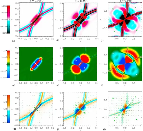
Figure 2.Contours of (a–c)|j|−|jMHS|, (d–f )p−pMHS, and (g–i)𝜔zin the planez=0.4across the separator, att=0.019tf(Figures 2a, 2d, and 2g),t=0.09tf
(Figures 2b, 2e, and 2h), andt=0.60tf(Figures 2c, 2f, and 2i). Asterisks, which initially lie on the edge of the diffusion region, as shown in Figure 1c, move at the
fast magnetoacoustic speed,cf(x,y,z,t). Over plotted on the bottom row of graphs are arrows (normalized to the maximum value of the magnitude of the
velocity in the domain att=0.60tf,|v|=6×10⁻³) that display the direction ofvxandvyin thez=0.4plane. As time increases, so do the dimensions of
the planes.
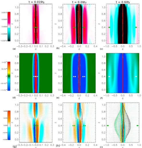
Cuts in thez=0.4plane are plotted in Figure 2 showing the behavior of the perturbed current, perturbed plasma pressure, and vorticity at three different times. In Figures 3 and 4, the cuts are taken at the same three times but are through the depth and across the width of the current layer, respectively. So the vertical axis for these graphs runs along thezaxis from the lower to the upper null. However, the current layer is twisted, so the horizontal axis changes with distance along the separator, such that it always goes through the current layer depth (Figure 3) or width (Figure 4), as required. On all these graphs, we have plotted asterisks, which at the start of the experiment are located in thez=0.4plane on the current contour|j|=jcrit, i.e., on the edge
of the diffusion region (shown in the equilibrium field in Figure 1c). We advect these asterisks through the depth and across the width of current layer in thez=0.4plane at the fast magnetoacoustic speed,cf, both
Figure 3.As for Figure 2, but instead showing the perturbations in a vertical surface that crosses the depth of the current layer at right angles to its width. Here
the arrows (normalized to the maximum value of the magnitude of the velocity in the domain att=0.60tf,|v|=6×10⁻³) display the direction ofv
randvzin
this plane in Figures 3g–3i. The arrows are colored black whered<0and are colored green whered>0.
dimensional, the waves do not have to move in a planar manner, which may explain the small discrepancies between the wavefronts and the asterisks.
4.1. Current and Pressure Perturbations
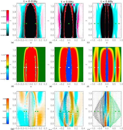
Figure 4.As for Figure 3, but instead showing the perturbations in a vertical surface that crosses the width of the current layer at right angles to its depth. Here
the arrows are colored black wherew<0and are colored green wherew>0and are normalized as in Figure 3. As in the previous figures, as time increases, so
do the dimensions of the planes.
when traveling across the width (Figure 4), but a deficit when traveling through the depth (Figure 3) of the current layer. The former are launched from the narrow edges of the current layer, as if from a point, and propagate outward, in a spherical-like manner, into the cusp regions, which in the MHS equilibrium, have larger pressure than the regions outside the cusps.
Outside the cusps, the latter type of perturbations are launched (i.e., carrying a deficit in pressure) from the comparatively wide edge of the current layer. These perturbations are more planar in nature; thus, they move linearly outward in a block from either side of the current layer. Figures 3a, 3d, 3g, 4a, 4d, and 4g show that the perturbations in current and pressure show a consistent behavior down the entire length of the separator current layer both through its depth and across its width. Remember though that the current layer is twisted, so these perturbations emanate out along the separator forming an expanded helical pattern. This is shown in a movie in the supporting information where isosurfaces of the pressure difference (drawn atp−p0=1×10⁻⁴
in yellow andp−p0= −1×10⁻⁴in blue) evolve through the reconnection experiment. In this movie, we are
looking down on the 3-D model, so only the negative null (red sphere) is seen, but the spines of both nulls are visible.
As these perturbed pulses travel farther from the reconnection site they are followed by a second set of pulses, which show the same basic behavior. These pulses are the ones that were launched at the same time as the lead pulses but traveled inward across the current layer, rather than outward from it. Naturally, therefore, for the wave pulses traveling outwith the cusps, the following planar pulses are very close behind the lead planar ones since they simply cross the (thin) depth of the current layer (Figures 2c, 2f, 2i, 3c, 3f, and 3i). In the cusps themselves, the following pulses that leave the narrow edges of the current layer have to cross the entire width of the current layer, and therefore, these are much further behind the leading point-like pulses (Figures 2c, 2f, 2i, 4c, 4f, and 4i).
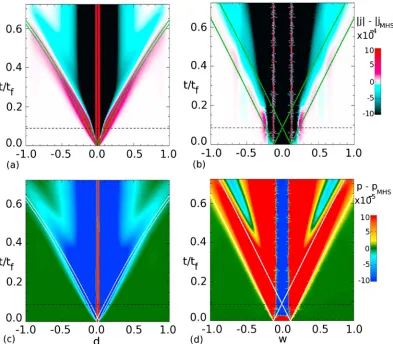
In Figure 5, time slices of the perturbed current and pressure through the depth and across the width of the current layer in thez=0.4plane are plotted. These show the wave pulses that travel from the edges of the diffusion region and match well with the overplotted lines that indicate the speed that fast magnetoacoustic waves, launched both inward and outward from the edges of the diffusion region, would travel at.
4.2. Steady Flows
In the wake of these perturbations, deficits of current exist both outside and within the cusps. Deficits of pressure exist only outwith the cusps, while enhancements of pressure inside the cusps form locally around the diffusion region (Figures 2–4). These regions do not move at a particular wave speed but expand out slowly throughout the duration of the experiment. Due to the loss of equilibrium within the separator current layer, the region surrounding the current layer, which is nonresistive, responds in order to try and regain force balance by trying to rebuild the current within the separator current layer. The forces present are basically the same as those found during the formation of the initial MHS equilibrium [Stevenson et al., 2015].
Outside the cusp regions, the inward directed magnetic pressure forces once more dominate over the out-ward directed plasma pressure force, generating an inflow toout-ward the separator current layer in this region. Inside the cusp regions, outward directed magnetic tension forces dominate over the inward directed plasma pressure forces causing an outflow. These flows are maintained because as soon as the current within the cur-rent layer strengthens to|j| = jcrit, diffusivity dissipates this current and thus prevents a static equilibrium
being formed. Instead, a system, which is close to a steady state, is created involving slow reconnection at the separator current layer (phase II of the reconnection process).
4.3. Infinite-Time Collapse
Figure 2a shows that the current enhancements on the separatrix surfaces are also perturbed, but there is no corresponding perturbation in pressure at this time (Figure 2d). Furthermore, the current along the separatrix surfaces is not decreased, as one might expect if these perturbations were the result of reconnection, but instead is increased.
Figure 5.Time slices of (a and b) the perturbed current and (c and d) the perturbed pressure plotted through the depth
(Figures 5a and 5c) and across the width (Figures 5b and 5d) of the current layer, in the plane atz=0.4. The black
dashed lines highlight where phase I ends and phase II begins. The green/white lines start on the edge of the current layer and represent a wave traveling at the fast magnetoacoustic speed.
residual forces that are very slowly increasing the current within the current layer and this is what continues to happen in our experiment here.
4.4. Vorticity and Velocity
In order to understand the nature of the flows created as a result of the reconnection, we consider both the vorticity and the velocity at three different times. Figures 2g–2i, 3g–3 i, and 4g–4i show the vorticity in the z = 0.4plane perpendicular to the separator, through the depth and across the width of the current layer, respectively. Overplotted on these graphs are arrows indicating the direction and size of the velocity in these cuts. The arrows are colored depending on their position: the arrows are colored black whered<0andw<0, and the arrows are colored green whered>0andw>0. We have colored the arrows this way so that the direction of the flow from a given side of the diffusion region is clearer.
Figures 2g–2i show a very similar pattern to the classical quadrupolar vortex scenario and stagnation flow found in 2-D X point reconnection regimes. The main difference is that instead of finding zero vorticity in the vicinity of the separator, an antiparallel flow is found associated with a clockwise (blue) rotating flow pattern (Figure 2i).
Not surprisingly, therefore, looking at the vorticity in the cut through the depth (Figure 3) and across the width (Figure 4) of the current layer, we see that the directions of the flows change with position along the separator. The velocity arrows indicate that the dominant flows are directed inward through the depth and outward across the width, for allz. However, superimposed on these are weak stagnation-type flow patterns.
Along the separator, in the cut through the depth (Figures 3g–3i), weak flows run toward both nulls from a point 0.6 times the length of the separator (as measured from the lower null). The location of this stagnation point, which corresponds to where the flows are purely directed inward to the current layer through the depth, does not appear to move over time. Its location is a result of the fact that the plasma pressure on the separator is greatest at this point in the MHS equilibrium, so the strongest magnetic pressure force must have existed at this location to counter the largest pressure force that would have been located there.
The cuts across the width of the current layer (Figures 4g–4i) show the opposite quadrupolar-vortex pattern close to the separator. This pattern shows that there are weak flows that run in from the nulls along the sep-arator to a point 0.4 times the length of the sepsep-arator (as measured from the lower null) at timet=0.019tf
(Figure 4g). This is the approximate center of the main stagnation outflow across the width of the current layer. It also corresponds to the point where the current is largest along the separator in the MHS equilibrium and thus where the outwardly directed tension force must have been highest. So as soon as the equilibrium is lost, a strong outflow in thez=0.4plane results.
Unlike the stagnation flow through the depth of the current layer, the stagnation-point flow across the width changes over time, such that at the time phase I ends, there seem to be two stagnation points on the separator. During phase II a single stagnation-type flow has reformed. It is not clear what the multiple stagnation-point flows indicate, but it is important to remember that at the transition between the two phases, very little reconnection, if any, is occurring since the slow, impulsive bursty reconnection phase has not yet formed.
5. Transport of Energy
We have already seen that the reconnection at the separator current layer leads to waves being launched in the system, from the edges of the diffusion site, due to the sudden lack of force balance. These waves travel out and cause the magnetic field and plasma to change, setting up flows in the system. In this section, we analyze the transport of magnetic, internal, and kinetic energy equations (as detailed inBirn et al., 2009 [2009]), integrated over volumes within our domain, in order to see what quantities these waves and flows carry with them.
To determine the quantities in the transport equations, we integrate each of them separately over subvolumes that increase in size within our domain. The nine volumes have sizes−(0.15+k∕10)≤x,y≤(0.15+k∕10), fork=0,1,2,…,8, and thezrange is fixed for all volumes at−0.2≤z≤1.2, since the waves and flows travel horizontally and not vertically out from the separator. Therefore, the smallest volume encloses the current layer, the second volume encloses the first volume and so on up to the largest volume, which is slightly smaller than the domain size in thexandydimensions. A cartoon of these volumes is shown in Figure 6a, where the volumes are colored black, purple, blue, lime, green, yellow, orange, and red as they increase in size. These volumes are shown drawn with the MHS equilibrium skeleton in Figure 6b to highlight the size of the boxes compared to the skeleton. Hence, in each plot of Figure 7, which shows the time evolution of the energy transport quantities, there are nine lines colored to match these volumes.
5.1. Transport of Magnetic Energy
The transport of magnetic energy equation states that
𝜕 𝜕t
(
B2
2𝜇0 )
= −𝜂j2− ∇⋅(E×B) −v⋅(j×B), (1)
wheretis time,B2is the square of the magnitude of the magnetic field (B=|B|),𝜇0is the magnetic
Figure 6.(a) Cartoon depicting the nine volumes over which the transport of energy equations are integrated. The volumes increase according to−(0.15+k∕10)≤x,y≤(0.15+k∕10)and−0.2≤z≤1.2shown by the colors black (k=0), purple (k=1), blue (k=2), cyan (k=3), lime (k=4), green (k=5), yellow (k=6), orange (k=7), and red (k=8), with the last box being just smaller than the size of the domain inxandy. (b) For context, the MHS equilibrium skeleton with boxes overdrawn.
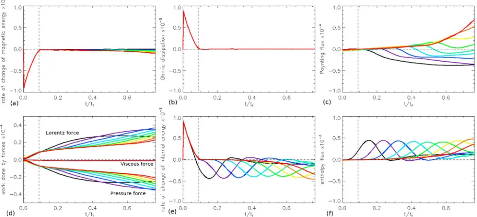
At the start of the experiment, there is an immediate drop in the rate of change of magnetic energy corresponding to the strong Ohmic dissipation during phase I, the fast-reconnection phase (Figure 7b). The integrated values of the Ohmic dissipation, which are of the order 10−3, are the same regardless of the size
of the volume (so only one line is visible) since the Ohmic dissipation occurs in the diffusion region, which is enclosed in all boxes. The Ohmic dissipation is fairly constant aftert = 0.09tf; the slow, impulsive bursty second phase.
The value of the Poynting flux, integrated over all volumes, is initially positive indicating that the waves are traveling out through the boundaries of our volumes (Figure 7c). The waves then cause the plasma to change, setting up flows in the system near to the original diffusion site. The flows bring Poynting flux in through the smaller volumes, from aboutt=0.16tfonward. However, the Poynting flux, carried out through the volumes by the waves, becomes relatively large the further out they travel (see the green to red lines in Figure 7c). Note, however, that the amount of Poynting flux is roughly 25 times smaller than the peak Ohmic dissipation in phase I.
The Lorentz force is working to try to regain force balance in the system from the moment the current in the separator current layer begins to be dissipated (positive values in Figure 7d). This figure shows that the work done by the Lorentz force, which is roughly of the order of 3×10⁻⁵, is acting out through the subvolumes
Figure 7.Quantities, plotted against time, of (a) the rate of change of the magnetic energy, (b) the Ohmic dissipation, (c) the Poynting flux, (d) the work done by the Lorentz, viscous, and pressure forces, (e) the rate of change of internal energy, and (f ) the enthalpy flux. The line color represents the different volumes over which these quantities have been integrated (cf. Figure 6). The black dashed vertical line highlights where phase I ends and phase II begins, and the black dashed horizontal line indicates zero.
lines, is directed outward from the diffusion site both within and outwith the cusp regions which are formed by the separatrix surfaces of the nulls. The magnetic pressure force is directed in toward the diffusion region within the cusps and outwith the cusps. Overall, these forces sum such that the work done by the Lorentz force is acting outward away from the diffusion region. The magnitude of this term is roughly 30 times smaller than the Ohmic dissipation term.
5.2. Transport of Internal Energy
Equation (2) is the transport of internal energy equation
𝜕
𝜕t(𝜌𝜖) =𝜂j
2− ∇⋅((p+𝜌𝜖)v) − (−v⋅∇p), (2)
where𝜌is the density and𝜖is the internal energy per unit mass.
Here we can write𝜌𝜖 = 3p∕2, since our closure equation is𝜖 = p∕𝜌(𝛾 −1), and𝛾 = 5∕3and therefore p+𝜌𝜖= 5p∕2. This equation states that the rate of change of internal energy is due to the Ohmic heating minus the enthalpy flux minus the work done by the pressure force. Figure 7e shows the rate of change of internal energy, which is of the order of 10−3, integrated over all nine volumes, throughout the experiment.
The initial sharp spike in this figure is due to the Ohmic heating (Figure 7b) as was seen in the energetics discussed inStevenson and Parnell[2015].
After this spike, the rate of change of internal energy decreases and becomes negative. A small traveling wave is seen moving out through all the subvolumes which comes from the enthalpy flux term (Figure 7f ). This term is of the order of 5×10⁻⁴and is half the size of the peak Ohmic dissipation during phase I.
5.3. Transport of Kinetic Energy
The transport of kinetic energy equation states that the rate of change of kinetic energy is equal to the work done by the Lorentz force plus the work done by the pressure force plus the work done by the viscous force minus the bulk kinetic energy flux
𝜕 𝜕t
( 𝜌v2
2 )
=v⋅(j×B) + (−v⋅∇p) +v⋅F𝜈− ∇⋅
( 𝜌v2
2 v )
, (3)
whereF𝜈=𝜈(∇2v+1
3∇(∇⋅v))is the viscous force.
The rate of change of kinetic energy is very small (∼5×10⁻⁷) throughout the reconnection experiment. This
is because the work done by the Lorentz and pressure forces (Figures 7d) are about equal in size but are of opposite sign (they are acting to regain force balance in the system after the dissipation of the current layer). Also, contributions from the work done by the viscous force (values close to zero in Figure 7d) and the bulk kinetic energy flux are very small (∼5×10⁻⁷) since the velocities in the system have small magnitudes.
Overall, we have found that there are five main terms which play a significant role in the transport of energy in our experiment. Ohmic heating plays the most significant role in our experiment, especially during phase I, converting magnetic energy into internal energy. This energy is then carried away from the diffusion region by the enthalpy flux, which is half the size of the Ohmic heating term and the Poynting flux, which is roughly 25 times smaller than the peak Ohmic heating. The final two important terms are the work done by the Lorentz and pressure forces, which are similar in magnitude, but act in opposite directions and are both about 30 times smaller than the Ohmic heating term.
6. Conclusions
In this paper, we have studied the properties of the waves and flows created due to spontaneous reconnec-tion at a 3-D separator current layer. We start with a system that is in MHS equilibrium everywhere save for very small forces at the current enhancements about the separator and separatrix surfaces. An anomalous diffusivity is applied such that reconnection only occurs at the separator current layer that twists about the separator.
The onset of the reconnection produces waves that propagate out from the edge of the diffusion site at the separator current layer. These waves only have small amplitudes, due to the relatively small reconnec-tion event that initiates them, and they travel at the fast magnetoacoustic speed (which in our high-beta experiment is approximately equal to the slow magnetoacoustic speed).
They carry the dissipated current away from the diffusion region and disperse as they travel. The nature of the waves has the same pattern in all planes perpendicular to the separator, which is basically the same as that found due to waves launched following reconnection at a 2-D X type null.
1. Planar-like waves that are twisted about the separator are launched from either side of the diffusion region and travel away from the separator current layer carrying current and causing a deficit in pressure. Equiva-lent waves are also launched inward through the depth of the current layer at the same time. These waves end up running closely behind the outwardly launched waves.
2. Point-like waves that again are twisted about the separator are launched outward from the narrow edges of the diffusion region. In any given plane perpendicular to the separator, these spread in a circular pattern carrying current away from the separator current layer and causing an enhancement in pressure. As above, point-like waves also travel inward across the width of the separator current layer, which is roughly 20 times the size of the depth; thus, these waves lag behind the outward waves.
These waves communicate the sudden loss of force balance within the separator current layer, and hence, in their wake magnetic and plasma forces are set up with the aim of restoring the equilibrium. As already explained byStevenson et al.[2015], an equilibrium in such a system with a separator involves a current enhancement about the separator, and thus, a velocity flow pattern is created, which brings in more flux from outwith the cusp regions to enhance the current at the separator. As soon as the current in the layer reaches the level ofjcritthe anomalous diffusivity dissipates it. This leads to a slow, impulsive bursty second phase of
The amplitude of the waves that result from the reconnection are small and of the order 10−4. They are,
however, much bigger (100 times) than those found in the 2-D high-beta experiment ofFuentes-Fernández et al.[2012a] which we believe is due to the third dimension permitting a larger current layer to be formed. To form an even larger current layer in our high-beta scenario, we could have start, prior to forming the MHS equilibrium, with an initial magnetic field that has either greater initial current or different magnetic field parameters (seeStevenson[2015] for full details). However, in the resulting MHS equilibrium the current layer was not resolved, and we were concerned that numerical diffusion had occurred, in some cases, before the MHS equilibrium could be formed. Also, the resulting waves were only marginally greater in amplitude. Lowering the value ofjcrit, the level above which the diffusivity is nonzero, would define a larger current layer, but this has the side effect of permitting reconnection within the current enhancements along the separatrix surfaces leading to more (complicated) wave pulses.
An analysis of the energy transport in the model shows that the Ohmic dissipation is about twice that of the enthalpy flux carried by the magnetoacoustic waves away from the reconnection site. In turn, the enthalpy flux is more than 10 times the work done by either the Lorentz or the pressure forces (which are basically the same size but cancel each other out since they work in opposite directions). The Poynting flux is also about 10 times smaller than the enthalpy flux. The dominance of the enthalpy flux over the Poynting flux is not surprising since our experiments are high beta (as shown inBirn et al.[2009]).
In order to compare our dimensionless results to those of a specific space plasma scenario, the speed of the waves generated by the reconnection can be scaled by the factorBn∕
√
𝜇𝜌n. In situ measurements by Double
Star have detected number densities ofnn = 10×106m−3and magnetic field strengths ofBn = 30nT at
the magnetopause [Trenchi et al., 2008]. Using a mean particle mass (this value has been calculated using magnetosheath abundances [Gloeckler and Hamilton, 1987] of the major magnetospheric ions [Rème et al., 2001]) ofm=1.07×mp, wherempis the mass of a proton, this number density corresponds to a mass density
of𝜌n = 1.8×10⁻²⁰kg m−3. In our experiment, the maximum dimensionless Alfvén speed in the outflow
regions isvA =1.6; thus, we find that the maximum Alfvén speed in our domain isvA = 320km s−1. This is
of the same order as the hybrid Alfvén speed,vAh=380km s−1, found between the magnetosheath and the
magnetosphere inKomar et al.[2013]. Note that in our model, the density in the outflow region decreases away from the separator and the magnetic field strength increases, so if our domain was larger, we would be able to measure greater values of the Alfvén speed than we have detailed here.
All the experiments discussed here can only be run until the traveling waves near the boundaries of the box. If it was possible to run these experiments for longer, then the viscous heating may increase sufficiently to become comparable with the observed Ohmic heating in this second phase. Furthermore, a low-beta system may also permit greater viscous heating. We plan, in a follow up paper, to investigate if this is the case.
References
Alexeev, I. I., D. G. Sibeck, and S. Y. Bobrovnikov (1998), Concerning the location of magnetopause merging as a function of the magnetopause current strength,J. Geophys. Res.,103, 6675–6684, doi:10.1029/97JA02863.
Arber, T. D., A. W. Longbottom, C. L. Gerrard, and A. M. Milne (2001), A staggered grid, Lagrangian-Eulerian remap code for 3-D MHD simulations,J. Comput. Phys.,171, 151–181, doi:10.1006/jcph.2001.6780.
Arzner, K., and M. Scholer (2001), Kinetic structure of the post plasmoid plasma sheet during magnetotail reconnection,J. Geophys. Res.,
106, 3827–3844, doi:10.1029/2000JA000179.
Birn, J., et al. (2001), Geospace Environmental Modeling (GEM) magnetic reconnection challenge,J. Geophys. Res.,106, 3715–3720, doi:10.1029/1999JA900449.
Birn, J., L. Fletcher, M. Hesse, and T. Neukirch (2009), Energy release and transfer in solar flares: Simulations of three-dimensional reconnec-tion,Astrophys. J.,695, 1151–1162, doi:10.1088/0004-637X/695/2/1151.
Biskamp, D. (2000),Magnetic Reconnection in Plasmas, Cambridge Univ. Press, Cambridge, U. K.
Borovsky, J. E. (2008), The rudiments of a theory of solar wind/magnetosphere coupling derived from first principles,J. Geophys. Res.,113, A08228, doi:10.1029/2007JA012646.
Borovsky, J. E. (2013), Physical improvements to the solar wind reconnection control function for the Earth’s magnetosphere,J. Geophys. Res. Space Physics,118, 2113–2121, doi:10.1002/jgra.50110.
Cao, J. B., X. H. Wei, A. Y. Duan, H. S. Fu, T. L. Zhang, H. Reme, and I. Dandouras (2013), Slow magnetosonic waves detected in reconnection diffusion region in the Earth’s magnetotail,J. Geophys. Res. Space Physics,118, 1659–1666, doi:10.1002/jgra.50246.
Close, R. M., C. E. Parnell, D. W. Longcope, and E. R. Priest (2005), Coronal flux recycling times,Sol. Phys.,231, 45–70, doi:10.1007/s11207-005-6878-1.
Dorelli, J. C., and A. Bhattacharjee (2008), Defining and identifying three-dimensional magnetic reconnection in resistive magnetohydrody-namic simulations of Earth’s magnetospherea),Phys. Plasmas,15(5), 056504, doi:10.1063/1.2913548.
Dorelli, J. C., and A. Bhattacharjee (2009), On the generation and topology of flux transfer events,J. Geophys. Res.,114, A06213, doi:10.1029/2008JA013410.
Acknowledgments
Drake, J. F., D. Biskamp, and A. Zeiler (1997), Breakup of the electron current layer during 3-D collisionless magnetic reconnection,
Geophys. Res. Lett.,24, 2921–2924, doi:10.1029/97GL52961.
Fuentes-Fernández, J., C. E. Parnell, and A. W. Hood (2011), Magnetohydrodynamics dynamical relaxation of coronal magnetic fields. II. 2D magnetic X-points,Astron. Astrophys.,536, A32, doi:10.1051/0004-6361/201117156.
Fuentes-Fernández, J., C. E. Parnell, A. W Hood, E. R. Priest, and D. W. Longcope (2012a), Consequences of spontaneous reconnection at a two-dimensional non-force-free current layer,Phys. Plasmas,19(2), 022901, doi:10.1063/1.3683002.
Fuentes-Fernández, J., C. E. Parnell, and E. R. Priest (2012b), The onset of impulsive bursty reconnection at a two-dimensional current layer,
Phys. Plasmas,072(7), 901, doi:10.1063/1.4729334.
Fujimoto, K., and R. D. Sydora (2008), Whistler waves associated with magnetic reconnection,Geophys. Res. Lett.,35, L19112, doi:10.1029/2008GL035201.
Galsgaard, K., and Å. Nordlund (1997), Heating and activity of the solar corona. 3. Dynamics of a low beta plasma with three-dimensional null points,J. Geophys. Res.,102, 231–248, doi:10.1029/96JA02680.
Galsgaard, K., E. R. Priest, and Å. Nordlund (2000), Three-dimensional separator reconnection—How does it occur?,Sol. Phys.,193, 1–16, doi:10.1023/A:1005248811680.
Gloeckler, G., and D. C. Hamilton (1987), AMPTE ion composition results,Phys. Scr. T.,18, 73–84, doi:10.1088/0031-8949/1987/T18/009. Gonzalez, W. D., and F. S. Mozer (1974), A quantitative model for the potential resulting from reconnection with an arbitrary interplanetary
magnetic field,J. Geophys. Res.,79, 4186–4194, doi:10.1029/JA079i028p04186.
Gosling, J. T., M. F. Thomsen, S. J. Bame, and C. T. Russell (1986), Accelerated plasma flows at the near-tail magnetopause,J. Geophys. Res.,91, 3029–3041, doi:10.1029/JA091iA03p03029.
Hara, H., T. Watanabe, L. K. Harra, J. L. Culhane, and P. R. Young (2011), Plasma motions and heating by magnetic reconnection in a 2007 May 19 flare,Astrophys. J.,741, 107, doi:10.1088/0004-637X/741/2/107.
Haynes, A. L., C. E. Parnell, K. Galsgaard, and E. R. Priest (2007), Magnetohydrodynamic evolution of magnetic skeletons,Proc. R. Soc. A,463, 1097–1115, doi:10.1098/rspa.2007.1815.
Hesse, M., and K. Schindler (1988), A theoretical foundation of general magnetic reconnection,J. Geophys. Res.,93, 5559–5567, doi:10.1029/JA093iA06p05559.
Hesse, M., N. Aunai, S. Zenitani, M. Kuznetsova, and J. Birn (2013), Aspects of collisionless magnetic reconnection in asymmetric systems,
Phys. Plasmas,20(6), 061210, doi:10.1063/1.4811467.
Hoshino, M., T. Mukai, T. Yamamoto, and S. Kokubun (1998), Ion dynamics in magnetic reconnection: Comparison between numerical simulation and Geotail observations,J. Geophys. Res.,103, 4509–4530, doi:10.1029/97JA01785.
Innes, D. E., B. Inhester, W. I. Axford, and K. Wilhelm (1997), Bi-directional plasma jets produced by magnetic reconnection on the Sun,
Nature,386, 811–813, doi:10.1038/386811a0.
Ko, Y.-K., J. C. Raymond, J. Lin, G. Lawrence, J. Li, and A. Fludra (2003), Dynamical and physical properties of a post-coronal mass ejection current sheet,Astrophys. J.,594, 1068–1084, doi:10.1086/376982.
Komar, C. M., P. A. Cassak, J. C. Dorelli, A. Glocer, and M. M. Kuznetsova (2013), Tracing magnetic separators and their dependence on IMF clock angle in global magnetospheric simulations,J. Geophys. Res. Space Physics,118, 4998–5007, doi:10.1002/jgra.50479.
Lau, Y.-T., and J. M. Finn (1990), Three-dimensional kinematic reconnection in the presence of field nulls and closed field lines,
Astrophys. J.,350, 672–691, doi:10.1086/168419.
Lin, J., Y.-K. Ko, L. Sui, J. C. Raymond, G. A. Stenborg, Y. Jiang, S. Zhao, and S. Mancuso (2005), Direct observations of the magnetic reconnection site of an eruption on 2003 November 18,Astrophys. J.,622, 1251–1264, doi:10.1086/428110.
Liu, R., J. Lee, T. Wang, G. Stenborg, C. Liu, and H. Wang (2010), A reconnecting current sheet imaged in a solar flare,Astrophys. J. Lett.,723, L2–L33, doi:10.1088/2041-8205/723/1/L28.
Longcope, D. W. (2001), Separator current sheets: Generic features in minimum-energy magnetic fields subject to flux constraints,
Phys. Plasmas,8, 5277–5290, doi:10.1063/1.1418431.
Longcope, D. W., and S. C. Cowley (1996), Current sheet formation along three-dimensional magnetic separators,Phys. Plasmas,3, 2885–2897, doi:10.1063/1.871627.
Longcope, D. W., and E. R. Priest (2007), Fast magnetosonic waves launched by transient, current sheet reconnection,Phys. Plasmas,14(12), 122905, doi:10.1063/1.2823023.
Longcope, D. W., and L. Tarr (2012), The role of fast magnetosonic waves in the release and conversion via reconnection of energy stored by a current sheet,Astrophys. J.,756, 192, doi:10.1088/0004-637X/756/2/192.
Milligan, R. O., R. T. J. McAteer, B. R. Dennis, and C. A. Young (2010), Evidence of a plasmoid-looptop interaction and magnetic inflows during a solar flare/coronal mass ejection eruptive event,Astrophys. J.,713, 1292–1300, doi:10.1088/0004-637X/713/2/1292.
Moore, T. E., M.-C. Fok, and M. O. Chandler (2002), The dayside reconnection X line,J. Geophys. Res.,107(A10), 1332, doi:10.1029/2002JA009381.
Nishizuka, N., H. Takasaki, A. Asai, and K. Shibata (2010), Multiple plasmoid ejections and associated hard X-ray bursts in the 2000 November 24 flare,Astrophys. J.,711, 1062–1072, doi:10.1088/0004-637X/711/2/1062.
Øieroset, M., T. D. Phan, R. P. Lin, and B. U. Ö. Sonnerup (2000), Walén and variance analyses of high-speed flows observed by Wind in the midtail plasma sheet: Evidence for reconnection,J. Geophys. Res.,105, 25,247–25,264, doi:10.1029/2000JA900075.
Parker, E. N. (1957), Sweet’s mechanism for merging magnetic fields in conducting fluids,J. Geophys. Res.,62, 509–520, doi:10.1029/JZ062i004p00509.
Parnell, C. E., A. L. Haynes, and K. Galsgaard (2008), Recursive reconnection and magnetic skeletons,Astrophys. J.,675, 1656–1665, doi:10.1086/527532.
Parnell, C. E., A. L. Haynes, and K. Galsgaard (2010), Structure of magnetic separators and separator reconnection,J. Geophys. Res.,115, A02102, doi:10.1029/2009JA014557.
Parnell, C. E., J. E. H. Stevenson, J. Threlfall, and S. J. Edwards (2015), Is magnetic topology important for heating the solar atmosphere?,
Philos. Trans. R. Soc. A,373, 20140264, doi:10.1098/rsta.2014.0264.
Paschmann, G., I. Papamastorakis, N. Sckopke, G. Haerendel, B. U. O. Sonnerup, S. J. Bame, J. R. Asbridge, J. T. Gosling, C. T. Russel, and R. C. Elphic (1979), Plasma acceleration at the Earth’s magnetopause—Evidence for reconnection,Nature,282, 243–246, doi:10.1038/282243a0.
Petschek, H. E. (1964), Magnetic field annihilation, inProceedings of the AAS-NASA Symposium on the Physics of Solar Flares, held 28–30 October, 1963 at the Goddard Space Flight Center, Greenbelt, Md., NASA Spec. Publ., vol. 50, edited by W. N. Hess, pp. 425–437, Natl. Aeronaut. and Space Admin., Sci. and Tech. Inf. Div., Washington, D. C.
Platten, S. J., C. E. Parnell, A. L. Haynes, E. R. Priest, and D. H. Mackay (2014), The solar cycle variation of topological structures in the global solar corona,Astron. Astrophys.,565, A44, doi:10.1051/0004-6361/201323048.
Pontin, D. I., and I. J. D. Craig (2006), Dynamic three-dimensional reconnection in a separator geometry with two null points,Astrophys. J.,
642, 568–578, doi:10.1086/500725.
Priest, E., and T. Forbes (Eds.) (2000),Magnetic Reconnection: MHD Theory and Applications, Cambridge Univ. Press, Cambridge, U. K. Priest, E. R., D. W. Longcope, and J. Heyvaerts (2005), Coronal heating at separators and separatrices,Astrophys. J.,624, 1057–1071,
doi:10.1086/429312.
Rème, H., et al. (2001), First multispacecraft ion measurements in and near the Earth’s magnetosphere with the identical Cluster ion spectrometry (CIS) experiment,Ann. Geophys.,19, 1303–1354, doi:10.5194/angeo-19-1303-2001.
Savage, S. L., G. Holman, K. K. Reeves, D. B. Seaton, D. E. McKenzie, and Y. Su (2012), Low-altitude reconnection inflow-outflow observations during a 2010 November 3 solar eruption,Astrophys. J.,754, 13, doi:10.1088/0004-637X/754/1/13.
Schindler, K., M. Hesse, and J. Birn (1988), General magnetic reconnection, parallel electric fields, and helicity,J. Geophys. Res.,93, 5547–5557, doi:10.1029/JA093iA06p05547.
Sonnerup, B. U. Ö. (1974), Magnetopause reconnection rate,J. Geophys. Res.,79, 1546–1549, doi:10.1029/JA079i010p01546. Sonnerup, B. U. Ö. (1979),Magnetic Field Reconnection, pp. 45–108, North-Holland, Amsterdam.
Sonnerup, B. U. O., G. Paschmann, I. Papamastorakis, N. Sckopke, G. Haerendel, S. J. Bame, J. R. Asbridge, J. T. Gosling, and C. T. Russell (1981), Evidence for magnetic field reconnection at the Earth’s magnetopause,J. Geophys. Res.,86, 10,049–10,067,
doi:10.1029/JA086iA12p10049.
Stevenson, J. E. H. (2015), On the properties of single-separator MHS equilibria and the nature of separator reconnection, PhD thesis, School of Math. and Stat., Univ. of St Andrews, Scotland.
Stevenson, J. E. H., and C. E. Parnell (2015), Spontaneous reconnection at a separator current layer: 1. Nature of the reconnection,J. Geophys. Res. Space Physics,120, doi:10.1002/2015JA021730.
Stevenson, J. E. H., C. E. Parnell, E. R. Priest, and A. L. Haynes (2015), The nature of separator current layers in MHS equilibria. I. Current parallel to the separator,Astron. Astrophys.,573, A44, doi:10.1051/0004-6361/201424348.
Swisdak, M., and J. F. Drake (2007), Orientation of the reconnection X-line,Geophys. Res. Lett.,34, L11106, doi:10.1029/2007GL029815. Takasao, S., A. Asai, H. Isobe, and K. Shibata (2012), Simultaneous observation of reconnection inflow and outflow associated with the 2010
August 18 solar flare,Astrophys. J. Lett.,745, L6, doi:10.1088/2041-8205/745/1/L6.
Trattner, K. J., J. S. Mulcock, S. M. Petrinec, and S. A. Fuselier (2007), Probing the boundary between antiparallel and component reconnection during southward interplanetary magnetic field conditions,J. Geophys. Res.,112, A08210, doi:10.1029/2007JA012270. Trenchi, L., et al. (2008), Occurrence of reconnection jets at the dayside magnetopause: Double Star observations,J. Geophys. Res.,113,
A07S10, doi:10.1029/2007JA012774.
Wang, T., L. Sui, and J. Qiu (2007), Direct observation of high-speed plasma outflows produced by magnetic reconnection in solar impulsive events,Astrophys. J. Lett.,661, L207–L210, doi:10.1086/519004.
Watanabe, T., H. Hara, A. C. Sterling, and L. K. Harra (2012), Production of high-temperature plasmas during the early phases of a C9.7 flare. II. Bi-directional flows suggestive of reconnection in a pre-flare brightening region,Sol. Phys.,281, 87–99, doi:10.1007/s11207-012-0079-5. Yokoyama, T., K. Akita, T. Morimoto, K. Inoue, and J. Newmark (2001), Clear evidence of reconnection inflow of a solar flare,Astrophys. J. Lett.,