Circular Scale of Time as a Guide for the Schrödinger Perturbation Process of a Quantum Mechanical System

(1)

ISSN Online: 2160-0503 ISSN Print: 2160-049X

DOI: 10.4236/wjm.2019.95009 May 16, 2019 113 World Journal of Mechanics

Circular Scale of Time as a Guide for the

Schrödinger Perturbation Process of a

Quantum-Mechanical System

Stanis

ł

aw Olszewski

Institute of Physical Chemistry, Polish Academy of Sciences, Warsaw, Poland

Abstract

We point out that a suitable scale of time for the Schrödinger perturbation process is a closed line having rather a circular and not a conventional straight-linear character. A circular nature of the scale concerns especially the time associated with a particular order N of the perturbation energy which provides us with a full number of the perturbation terms predicted by Huby and Tong. On the other hand, a change of the order N—connected with an increased number of the special time points considered on the scale—requires a progressive character of time. A classification of the perturbation terms is done with the aid of the time-point contractions present on a scale characte-ristic for each N. This selection of terms can be simplified by a partition pro-cedure of the integer numbers representing N−1_{. The detailed calculations} are performed for the perturbation energy of orders N =7_and N=8_.

Keywords

Quantum Mechanics, Schrödinger’s Perturbation Process, Accuracy of a Circular Scale of Time in the Perturbation Calculations

1. Introduction

The scale of time, which is well known in everyday life and in science, too, is a product of a long experience. As far as we can distinguish the later events from the earlier ones, we organize the idea of time as a parameter which allows us to get an insight into the degree of the past, or future, connected with our observations.

In effect a tool to classify the events, and the time distances between them, is established. Conventionally this is done with the aid of an infinite scale extended between an infinite past—say representing the negative coordinates—and a sim-How to cite this paper: Olszewski, S.

(2019) Circular Scale of Time as a Guide for the Schrödinger Perturbation Process of a Quantum-Mechanical System. World Journal of Mechanics, 9, 113-145. https://doi.org/10.4236/wjm.2019.95009

Received: March 25, 2019 Accepted: May 13, 2019 Published: May 16, 2019

(2)

DOI: 10.4236/wjm.2019.95009 114 World Journal of Mechanics ilar scale—say having the positive coordinates—representing the future:

. t

−∞ < < ∞ ₍₁₎

The distances between the time points on the scale can be measured with a smaller or larger accuracy. These distances provide us with separations between different time points.

In practice the Schrödinger’s quantum mechanics—developed in course of 1920’s [1] [2] [3] [4]—has not much to do with the intervals of time. Its main idea was rather to distinguish between the stationary states of the chosen pieces of matter. Such pieces are described with the aid of the stationary eigenenergies and eigenfunctions, both kinds of parameters being independent of time. Con-cretely the classical Hamiltonian function of a chosen object is transformed into its operator form, and the integration of the classical Hamilton equations is re-placed by a study of a differential eigenequation of the form

ˆ _.

Hψ =Eψ

₍₂₎ Here

H

ˆ

is the Hamiltonian operator represented by a sum of the kinetic and potential operators

kin pot

ˆ ˆ _{ˆ ,}

H E= +E

(3) so—for a single particle system—

(

2 2 2

)

kin 1

ˆ _ˆ _ˆ _{ˆ ,}

2 x y z

E p p p

m

= + +

(4)

( )

pot

ˆ ˆ _,

E =V r =V r

₍₅₎

ψ is the eigenfunction called the wave function of an object, say a particle sub-mitted to an external field having the potential V, symbol r is the position vector, E is the energy eigenvalue.

Because of

ˆx , ˆy , ˆz ,

p i p i p i

x y z

∂ ∂ ∂

= − = − = −

∂ ∂ ∂

  

(6) the momentum operator in (4) is of a differential character, whereas (5) represented by a function of the particle (object) position r, is of a multiplicative nature.

The problem is that even in relatively simple physical cases the eigenequation (2) is difficult to solve. By solution we understand a set of the eigenenergies

1, , ,2 3

E E E E= _

₍₇₎ and eigenfunctions

1, , ,2 3

ψ ψ ψ ψ= _

₍₈₎ which satisfy (2). Only in very few physical cases equation (2) can provide us with simple solutions (7) and (8). The (7) are considered to be real energies of the system’s quantum states, the (8) are the wave functions suitable in calculat-ing other physical observables than energy.

(3)

dege-DOI: 10.4236/wjm.2019.95009 115 World Journal of Mechanics nerate one.

Schrödinger was certainly aware about the difficulties connected with the so-lution of his Equation (2); see [3]. His proposal became to calculate the solutions of a rather complicated (2) with the aid of solutions of a less complicated equa-tion

( ) ( )0 0 ( ) ( )0 0

ˆ _,

H ψ =E ψ _(2a) having the potential _V0

( )

_r _{more simple than}_V

( )

_r _{in (2). The potentials}

difference

( )

( )0

_{( )}

per per

ˆ

V =V =V r −V r ₍₉₎

is called the perturbation potential, or simply a perturbation. In order to obtain possibly accurate results Schrödinger developed a formalism in which the solu-tions of (2) can be expressed with the aid of solusolu-tions of (2a). In this process—beyond of the solutions of (2a)—the matrix elements of the kind

( )0 _Vper ( )0

α β

ψ ψ

(10) are also involved.

A more easy treatment of the perturbation does concern the calculation of the energies of Equation (2) with the aid of solutions of Equation (2a) obtained in case of a non-degenerate case. Nevertheless an accurate calculation of these energies requires a complicated superposition of the solutions of (2a), as well as calculation of the matrix elements in (10). In principle these calculations were performed with no reference to the parameter of time; see Sec. 2.

The aim of the present paper is to point out that an introduction of the time scale—which has, however, a nature different than the well-known scale charac-terized by the formula (1)—provides us with a rather spectacular simplification of the original Schrödinger’s perturbation scheme.

2. Outline of the Time-Independent Perturbation Theory of

a Non-Degenerate Quantum State

A characteristic point is that Schrödinger obtained the solution of his perturbed equation without any reference to time [3]. An outline of a more modern time-independent perturbation theory is given, for example, in [5]. In the case of a non-degenerate quantum system let the unperturbed eigenequation

( ) ( )0 0 ( ) ( )0 0

ˆ _n _n _n

H ψ =E ψ

₍₁₁₎ be considered as solved. In principle we have an infinite set of the quantum numbers n for wnich the eigenequation (11) does hold. The number of the ei-genfunctions and eigenenergies of the perturbed eigenequation

( )

(

per

)

0

ˆ ˆ

H λ ψ = H +λV ψ =Eψ

(12) let be also infinite.

(4)

DOI: 10.4236/wjm.2019.95009 116 World Journal of Mechanics the following series expansions

( )

( )0 ( )1 2 ( )2

n n n n

ψ λ =ψ +λψ +λ ψ +_

(13) and

( )

( )0 ( )1 2 ( )2

n n n n

E λ =E + ∆λ E + ∆λ E +₍₁₄₎ and look for the solution of (12) in terms of the functions

( )0_, ( )1_, ( )2_,

n n n

ψ ψ ψ ₍₁₅₎ and numbers

( )0 _, ( )1_, ( )2_,

n n n

E ∆E ∆E _₍₁₆₎

which make (12) valid for any λ_{from the interval} 0< <λ 1. The function combined on the right of (13), viz.

( )0 ( )1 ( )2 ( )N

n n n n n

ψ =ψ +ψ +ψ +_+ψ

₍₁₇₎ is called the perturbed wave function of state n presented with the accuracy to the perturbation order N, whereas the numbers entering on the right of (14), viz.

( )0 ( )1 ( )2 ( )N

n n n n n

E =E + ∆E + ∆E ++ ∆E ₍₁₈₎

give the perturbed energy of state n also with the accuracy of the perturbation order N.

By assuming the convergence of the series in (13) and (14), an increase the order number N applied in the sequence

1, 2, 3, ,



N

₍₁₉₎ improves the accuracy of solutions presented in (13) and (14).

Physically as a more easy accessible and more interesting parameter, is consi-dered the perturbed energy (14). Huby and Tong presented the number of the kinds of terms necessary to obtain the successive components

( )1_, ( )2_, ( )3_, ( )N _,

E E E E

∆ ∆ ∆ ∆

₍₂₀₎

entering the Schrödinger series for the energy perturbation of any non-degenerate state n; see [6] [7]. This number is expressed as a function of N by the formula

(

)

(

)

2 2 !_.

! 1 !

N

N S

N N

− =

− (21)

For low N the numbers SN are also rather small, for example

1 1, 2 1, 3 2, 4 5, 5 14, 6 42,

S = S = S = S = S = S = _

₍₂₂₎

It should be noted that the kinds of the perturbation terms entering the set of N

S do not depend explicitly on state n, but they depend solely on N. Any kind of terms is, in its turn, a combination of the matrix elements of the perturbation potential with the unperturbed wave functions ( )0

α

ψ and ( )0

β

ψ _{, given in (10).} Another dependence of the terms is due to the differences of the unperturbed energy ( )0

n

(5)

ener-DOI: 10.4236/wjm.2019.95009 117 World Journal of Mechanics gies _E( )0

α , Eβ( )0 , Eγ( )0 , i.e.

( )0 ( )0_, ( )0 ( )0_, ( )0 ( )0_,

n n n

E −Eα E −Eβ E −Eγ ₍₂₃₎

As a rule the differences (23) enter the denominators of the perturbation terms, so there should be satisfied the relations

,

n

α

≠

β

≠

γ

≠

_

₍₂₄₎

etc.; see e.g. [8] for further details.

For N>2_{numerous terms entering}S_N composed of (10), (23) and (24) can be submitted to infinite summations over the states indicated on the left of (24).

In practice the way of deriving the sets of SN terms necessary for the Schrödinger perturbation formalism indicated above becomes a complicated task. Concurrent methods, obtained mainly without inclusion of the time para-meter, are given in [9]-[17]. The computational applications performed with the aid of these methods seem to not provide us with a complete formalism suitable for a large perturbation order N. One of the by-products of the present paper is to make the perturbation method for large N to be more simple than before.

3. Feynman’s Time-Dependent Formalism Referred to the

Schrödinger Perturbation Theory

Feynman diagrams including the time variable became a well-known tool in representing the quantum phenomena of different kind [18] [19] [20]. They could be applied also in the case of the Schrödinger perturbation calculation. A fundamental difficulty of such a treatment comes from an enormous inflation of the number of diagrams which had to be considered in case of a large perturba-tion order N. For, according to the Feynman formalism, we should calculate and combine the results of

(

1 !

)

N

P = N−

(25) diagrams in order to obtain the energy expression equivalent to the SN terms entering the Schrödinger theory.

It is evident that

N N

P =S

₍₂₆₎

for N =1,2_{, and 3, but already for} N =4_{we have}

4 6 4 5.

P = >S =

₍₂₇₎

It is easy to check that for N3 we have PN SN. For example for 20

N= _{we obtain}

17 20 19! 1.23 10

P = ≅ ×

₍₂₈₎ and

9 20 1.77 10 .

(6)

DOI: 10.4236/wjm.2019.95009 118 World Journal of Mechanics N N

P S ₍₃₀₎

increases systematically with N tending to a huge number.

But the Feynman theory was based on a linear time scale represented by the interval given in formula (1). We demonstrate—in the remainder part of the paper—that a different kind of the time scale, namely that having a circular-like character, can lead precisely to the diagrams and, in consequence, the energy terms dictated by the Schrödinger perturbation calculus.

4. Scale of Time Suitable for the Schrödinger Perturbation

Formalism, Its Contraction Points and Side Loops

Our idea is to replace a tedious calculation of the perturbation energy attained with the aid of solving the perturbed Schrödinger eigenequation by an imme-diate production of the perturbed energy terms due to an application of a suita-ble scale of time; see Figures 1-4.

According to Leibniz [21] [22] [23] time is an ordering parameter for the events occurring in the nature. A reference to the Leibniz concept of time as a merely successive order of things can be done also in connection of a discussion of the Mach’s principle and the structure of dynamical theories [24] [25] [26].

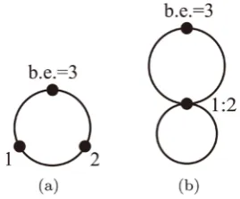
[image:6.595.305.440.569.681.2]

Figure 1. Time scale for the perturbation order N=1. The beginning-end point is 1.

Figure 2. Time scale for the perturbation order N=2. Beyond of the beginning-end point 2 there exists also point 1 on the scale. No contraction between 1 and 2 is admissible.

(7)

DOI: 10.4236/wjm.2019.95009 119 World Journal of Mechanics

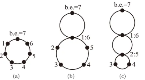
Figure 4. Time scale for the perturbation order N=7. Beyond of the beginning-end point 7 there exist also points 1, 2, 3, 4, 5 and 6. They are free on the diagram (a), but can form—for example—a maximal side loop for N=7 due to contraction 1: 6 [diagram (b)] or a cascade of loops [diagram (c)] due to contractions 1: 6 and 2 : 5.

In case of the perturbation calculation, the Leibniz idea suggests to choose an appropriate scale of time, so it will be helpful to represent the results of the per-turbation process. A necessary scale for any perper-turbation order N occurs to be a circular-like scale. This implies that N points of time—representing N successive collisions of the quantum system with the perturbation potential (9)—are present on a topological circle. One of these points, say the Nth point, let be the beginning-end point of the scale, called henceforth the main scale, or loop, of time. The remainder N−1_{time points on the scale can be left either free, or} submitted to contractions.

The contractions of the time points done on the main scale lead to the side loop, or loops, of time. Since it occurs that the Nth point should be excluded from contractions, a maximal size of the loop created from the main loop of the N points of time is given by the contraction between the time points 1 and

1

N− _{. This contraction is labelled by}

1:N−1.

₍₃₁₎ Beyond of the maximal loop of (31), a set of the minimal loops due to con-tractions

1: 2, 2 : 3, 3: 4, ,

_

N

−

2 :

N

−

1

₍₃₂₎ can be also created. We can have still the intermediate side loops like

1: 3, 2 : 4, 3: 5, ,

_

N

−

3:

N

−

1,

₍₃₃₎ or other loops larger than those due to contractions in (33).

Beyond of single contractions listed in (31)-(33), also multiple contractions of the time points like

1: 2 : 3, 2 : 4 : 5, 2 : 4 : 7,

₍₃₄₎ or

[image:7.595.261.497.68.199.2]

(8)

DOI: 10.4236/wjm.2019.95009 120 World Journal of Mechanics considered N. Moreover, the combined contractions of the time points like

1: 2 4 : 5



₍₃₅₎

may come also into play. A general rule is that the time loops due to the accepta-ble contractions should not cross. This means that, for example, the combined contraction due to the pair

1: 4 2 : 5



₍₃₆₎ is not admissible.

A fundamental effect is that a full set of acceptable contractions for a consi-dered order N gives precisely the number SN of the Schrödinger perturbation terms predicted by the formula (21) for that N; no superflous neither lacking terms do occur. This is checked for the orders between N=1_and N =7_in the earlier papers by the author [25-34]. A full set of diagrams necessary for

6

N= _{is given in}_[25]_{, a similar set for} N =7_enters_[34]_{. In the present paper} the perturbation energy of the order N=8_{is also examined from the same} point of view giving a similar agreement of the results; see Sec. 9.

5. Concentrations of the Contraction Points and Their Use

The concentration of a contraction point is equal to the number of the loops of time which meet together in that point. Evidently, if the contraction point is lo-cated on the main loop of time, one of the loops met in that point is the main loop itself. The other loops created by the time contractions on the main loop are called the side loops. An advantage to operate with the concentrations of loops is that they allow us to express the perturbation results in a more compact form than could be expected before.

This is so because the concentrations which are characteristic for a given N can be referred directly to partitions of the number N−1. In the next step the knowledge of partitions does lead to the number of the perturbation terms and the formulae for these terms. The effect of partitions and their connections with the contraction points will become evident in the computational practice giving the SN Schrödinger terms for N=7 and N=8; see Sec. 9.

(9)

DOI: 10.4236/wjm.2019.95009 121 World Journal of Mechanics presented both in Sec. 6 and Sec. 9.

6. Notation Applied to Represent

the Energy Perturbation Terms

Only for the perturbation orders N=1_and N =2_{the side loops for the} main loop of time do not exist. But any SN term for N >2 is a product of energy contributions due to the main loop of time and those due to the side loops, respectively.

The contributions due to the side loops are easy to access from contractions of the time points and will be discussed first. Any contraction

:

α β

₍₃₇₎

where as a rule we have

α β

<

_(37a)

provide us with the energy multiplier equal to the energy correction .

Eβ α−

∆ ₍₃₈₎

The difference

β α

−

₍₃₉₎

indicates the perturbation order of energy contributed by the side loop represented by ∆E_{. In result, when the difference indicated in (39) is larger} than 2, we have more than one Schrödinger perturbation term represented by the side loop, for

1.

Sβ α− > ₍₄₀₎ The contribution to energy due to the main loop of time depends on the number and situation of the time points present on that loop. When no contrac-tions are present for the time points on the loop, the loop has N time points on it and gives the energy term in the form

VPVPVPVP PV . (41) Such loop carries N symbols V and N−1_symbols_P_.

Evidently for N=1_no_P_{symbol enters (41) and we obtain a single term for} the perturbation energy equal to

per

1.

V = n V n = ∆E

₍₄₂₎

For the order N=2_{we have no side loops and the perturbation energy is} represented by the formula

2.

VPV = ∆E ₍₄₃₎

The symbol P within the brackets on the left of (43) represents a reciprocal value of the energy difference, viz.

( )0 ( )0

1 _,

n p

P

E E

=

−

(44)

(10)

per _, per _,

n V p p V n _(44a)

and submitted to summation process over the dummy state index p. In effect

( )0 ( )

p

0

er per

.

p n _n _p

n V p p

E n V

E V PV

≠ =

−

∑

(45)

The meaning similar to the term (45) does prolongate to any perturbation term given by the main loop of time carrying no contraction points. For example for N=3_{such term is represented by}

( )0 ( ) ( ) ( )

per p r r

0 0

e p

0 e

.

p nq n _n _p _n _q

n V p p V q q V E E E E

n VPVPV

≠ ≠

=

 ₋   ₋ 

   

∑∑

(46)

This formula has two P and two dummy indices (p and q) for summation over the quantum states with exclusion of state n which is submitted to perturbation. It is easy to extend (46) to an arbitrary order N.

More complicated contributions to energy due to the main loop occur in case when the side loops are also present. For N=3_{the only possible contraction} of the time points is

1: 2.₍₄₇₎ Evidently the side loop created by (47) does provide us with the term

1,

V = ∆E

_(47a)

however our task is to present also a contribution due to the main loop of time. In this case contraction (47) transforms the term (46)—having no contrac-tions—to the formula

( ) ( )

per per

2

0 0

2 _.

p n

n p

n V p p V n

VP

E V

E

≠ =

 − 

 

∑

(48)

The whole perturbation energy due to contraction (47) is represented by the product of (47a) and (48) taken with a minus sign:

2

1: 2→ − VP V V

(49) because we have an even number of terms entering the product in (49); an odd number of terms would give a positive sign. A characteristic point is that the to-tal number of P and V entering the term in (49) remains the same as it does exist in the term (46): there are two P and three V together.

Another situation can be when the non-neighbouring time points, say 1 and 3, enter contraction

1: 3.₍₅₀₎ This may occur for the perturbation order equal at least to N =4_{, so the last} time point 4 is the beginning-end point on the scale and does not enter into contractions.

(11)

DOI: 10.4236/wjm.2019.95009 123 World Journal of Mechanics ( ) ( ) ( ) ( ) ( ) ( )

per per per per

0 0 0 0 0 0

p nq nr n _n _p _n _q _n _r

n V p p V q q V r r V n VPV

E E E E E PVPV

E

≠ ≠ ≠

=

 −   −   − 

     

∑∑∑

(51)

whereas the contraction (50) implies the side loop having point 2 as free on it. This makes the energy contribution due to the side loop equal to

2

VPV = ∆E

₍₅₂₎

But the main loop of time having a contraction point (50) on it changes its contribution to the perturbation energy. Together with the beginning-end point of time the loop becomes similar to that representing the term (52), however the presence of the contraction point (50) implies the loop contribution to energy equal to

( ) ( )

per per

2

0 0

2 _.

p n

n p

n V p p V n

VP

E V

E

≠ =

 − 

 

∑

(53)

In effect the perturbation term due to contraction (50) is equal to product of (52) and (53):

2

2 .

E VP V

−∆

(54) The minus sign in (54) is dictated by the presence of an even number of terms entering the final product.

The notation procedure indicated above can be extended to any perturbation order N.

7. Time-Point Contractions on a Circular Scale and a Check

of Validity of the Energy Terms Contributed by the

Side-Loops of Time

Let us begin with a maximal side loop presented by the time point contraction in (31). Because the number of free points of time present on the side loop in (31) is

1 1

2,

N

′ = − − = −

N

₍₅₅₎ the energy contributed by the side loop due to (31) is equal to

2.

N

E −

∆ ₍₅₆₎

This energy has to be joined with the energy contribution given by the main loop of time which—due to contraction (31)—possess only two points of time: the beginning-end point and the contraction point (31). It should be noted that the presence of the beginning-end point does not give any contribution to the perturbation energy, for such contribution can be given only by a loop of time.

In effect of the contraction point of two loops, they are joined together. This implies that the energy term of the main loop should have the term

2

(12)

DOI: 10.4236/wjm.2019.95009 124 World Journal of Mechanics term; see (52). In effect the main loop makes the whole contribution of the con-traction (31) to the perturbation energy equal to

2

2.

N

VP V E −

− ∆

(58) A formal check of validity of the energy expression given in (58) is simple: since the perturbation energy concerns order N, it should have the total number of P in the perturbation expression equal to N−1_{and the number}_V_{is equal to} N. Respectively, the perturbation energy in (51) contains the number of P equal to N−3_{and that of}_V_{equal to} N−2_{. The multiplier}

2

VP V

(59) present in (58) supplies the lacking number of P and V in the term ∆EN−2 to

the required number of P and V in an energy term belonging to ∆EN. The same reasoning can be applied to any contraction of the time points

1,2,3, , N−1₍₆₀₎ entering the time scale useful for calculating the perturbation energy of the order N.

Examples of such calculations are presented in the earlier papers; see e.g. [33] [34]. The number of the time points which can be submitted to contractions for a given N is N−1_{; evidently different contractions can give different} concentra-tions at the contraction points. The point present on the scale having no con-tractions has concentration 1, a maximal concentration of the N−1_time points is evidently N−1_.

The same number N−1_{is equal to the number of}_P_{’s present in any term of} the Schrödinger perturbation energy; evidently for N=1_{we have no}_P_present in the perturbation term.

8. Systematic Time-Dependent Approach to the Schrödinger

Perturbation Method. Partitions of the Number N

−

1 and

the Time Point Contractions

A fundametnal process of quantum mechanics is a change of a given system upon the action of a perturbation which—in its character—can be independent of time. To calculate the result of such a change on a non-degenerate system the Schrödinger perturbation formalism—represented by the sets of terms labelled by their order numbers N—is usually applied.

(13)

DOI: 10.4236/wjm.2019.95009 125 World Journal of Mechanics an almost automatic way.

All possible partitions of the number N−1_{lead to respective time-point} contractions necessary for calculating the perturbation terms belonging to that N. Certainly the time points entering contractions are dependent on the position of a given partition number in the sum equal to N−1_{. In this way we obtain a} full set of necessary contractions for a given number N−1_.

For example for N=3_{we have} N− =1 2_{and the only set of the} accepta-ble contractions is reduced to a single contraction

1: 2=N−2 :N−1₍₆₁₎ represented by a partition number of N−1_{equal to 2. But there exists also the} partition

1 1

_(61a) without contractions.

For N=4_{we have the contractions}1: 2 and 2 : 3 represented by parti-tions

2 1

1 2.

(62) Here the time point 3 and time point 1 remain free in the first and second row of (62), respectively. A full set of partitions for N− =1 3_becomes

1 1 1 2 1 1 2

3;

(63)

the partition 3 does represent the contractions 1: 2 : 3 and 1: 3. For N=5_{we obtain the partitions}

(

)

4

1

1 1 1 1→no contractions points 1,2,3,4 free ;S =1₍₆₄₎

2 2 1

2 1 1 1: 2, points 3,4 free;→ S S =1

₍₆₅₎

1 2 1

1 2 1→2 : 3, points 1,4 free;S S S =1

₍₆₆₎

2 1 2

1 1 2→3: 4, points 1,2 free;S S =1₍₆₇₎

1 2

2 2→1: 2, 3: 4;S S =1₍₆₈₎

3 1

3 1 1: 3,1: 2 : 3; point 4 free;→ S S =2₍₆₉₎

1 3

1 3→2 : 4, 2 : 3: 4; point 1 free;S S =2₍₇₀₎

4

4→1: 4,1: 2 : 4,1: 3: 4,1: 2 : 3: 4,1: 4 2 : 3;_ S =5.₍₇₁₎ A characteristic point is that the S-like results are equal to the number of con-tractions; an exception is the first term [see (64)] where the absence of contrac-tions is associated with all particontrac-tions equal to 1. A total value of the sum of the S-products on the left of (64)-(71) is equal to:

4 2 2 2

1 2 1 1 2 1 1 2 2 3 1 1 3 4

5

1 1 1 1 1 2 2 5 14 .

S S S S S S S S S S S S S S S

+ + + + + + +

(14)

DOI: 10.4236/wjm.2019.95009 126 World Journal of Mechanics Therefore a set of partitions of N− =1 4_{gives the} S₅ perturbation terms. A similar situation does repeat for N=6_{which gives} N− =1 5_{; the} parti-tions are

(

)

5

1

1 1 1 1 1 points 1,2,3,4,5 free ;S =1

(73)

(

)

3

2 1

2 1 1 1 1: 2, 3,4,5 free ;→ S S =1

(74)

(

)

1 2 1

1 2 1 1 2 : 3, 1,4,5 free ;

→

S S S

=

1

(75)

(

)

2

1 2 1

1 1 2 1→3: 4, 1,2,5 free ;S S S =1

(76)

(

)

3

1 2

1 1 1 2→4 : 5, 1,2,3 free ;S S =1

(77)

2 1 2

1 2 2 2 : 3 4 : 5;

→

_

S S

=

1

₍₇₈₎

2 1 2

2 1 2→1: 2 4 : 5; S S S =1₍₇₉₎

2 2 1

2 2 1 1: 2 3: 4;

→



S S

=

1

₍₈₀₎

2 1 3

1 1 3→3: 5, 3: 4 : 5;S S =2

₍₈₁₎

1 3 1

1 3 1→2 : 4, 2 : 3: 4;S S S =2

₍₈₂₎

2 3 1

3 1 1 1: 3,1: 2 : 3;→ S S =2 ₍₈₃₎

4 1

4 1 1: 4,1: 2 : 4,1: 3: 4,1: 2 : 3: 4,1: 4 2 : 3;→  S S =5

₍₈₄₎

1 4

1 4→2 : 5, 2 : 3: 5, 2 : 4 : 5, 2 : 3: 4 : 5, 2 : 5 3: 4;_ S S =5₍₈₅₎

5

5→1: 5,1: 2 : 5,1: 3: 5,1: 4 : 5,1: 2 : 3: 5,1: 3: 4 : 5,1: 2 : 3: 4 : 5;S =14;₍₈₆₎ The total sum obtained from the 14 S like terms on the right is equal to

5 3 2 2 3 2 2

1 2 1 1 2 1 1 2 1 1 2 1 2 2 1 2 2 1

2 2

1 3 1 3 1 3 1 2 3 3 2 1 4 4 1 5

6

1 1 1 1 1 1 1 1 2 2 2 2 2 5 5 14 42 .

S S S S S S S S S S S S S S S S S S S S S S S S S S S S S S S S S S

S

+ + + + + + +

+ + + + + + + +

= + + + + + + + + + + + + + + + = =

(87)

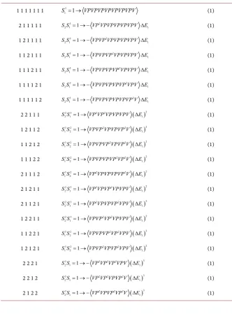
Having the contraction data in (73)-(86) it becomes easy to construct the per-turbation terms belonging to N=6_{. These terms are respectively:}

1 1 1 1 1

→

VPVPVPVPVPV

,

(88)

2

1

2 1 1 1→ − VP VPVPVPV E∆ ,

(89)

2

1

1 2 1 1→ − VPVP VPVPV E∆ ,

(90)

2

1

1 1 2 1→ − VPVPVP VPV E∆ ,

(91)

2 1

1 1 1 2→ − VPVPVPVP V E∆ ,

(92)

(

)

2

2 2

1

1 2 2→ VPVP VP V ∆E ,

(93)

(

)

2

2 2

1

2 1 2→ VP VPVP V ∆E ,

(94)

(

)

2

2 2

1

2 2 1→ VP VP VPV ∆E

(95)

(

)

2 2

2 3

1

1 1 3 ,

,

VPVPVP V E VPVPVP V E

→ − ∆

∆

(15)

(

)

2 2 2 3 1

1 3 1 ,

,

VPVP VPV E VPVP VPV E

→ − ∆ ∆ (97)

(

)

2 2 2 3 1

3 1 1 ,

,

VP VPVPV E VP VPVPV E

→ − ∆ ∆ (98)

(

)

2 2 2 1 2 3 2 1 1

3 2 ,

,

VP VP V E E

VP VP V E E

→ ∆ ∆

− ∆ ∆

(99)

(

)

2 2 1 2 2 1 1 3 2

2 3 ,

,

VP VP V E E

VP VP V E E

→ ∆ ∆

− ∆ ∆

(100)

( )

(

) ( )

2 3 3 2 1 3 1 2 3 4 1

4 1 2

1 1 1

VP VPV E VP VPV E E VP VPV E E VP VPV E

→ − ∆ ∆ ∆ ∆ ∆ − ∆

(101)

( )

(

) ( )

2 3 3 2 1 3 1 2 3 4 1

1 4 2

1 1 1

VPVP V E VPVP V E E VPVP V E E

VPVP V E

→ − ∆ ∆ ∆ ∆ ∆ − ∆

(102)

( )

(

) ( )

( )

2 4 3 1 3 2 3 2 3 3 1 5 5 2 1 2

VP V E VP V E E

VP V E

VP V E E

→ − ∆ ∆ ∆ ∆ ∆ ∆

(

)

( )

(

) ( )

(

) ( )

2 4 1 2 4

1 2 1

2 4 2 1 4 5 1 1 1 1 1

VP V E E VP V E E E VP V E E VP V E

− ∆ ∆ − ∆ ∆ ∆ − ∆ ∆ ∆

(103)

The numbers in brackets represent the quantity of the perturbation terms in a given rows.

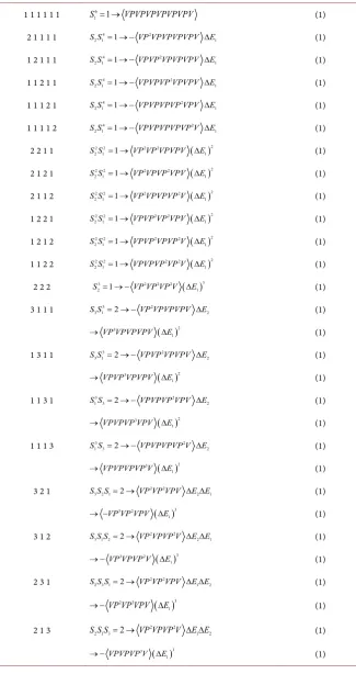
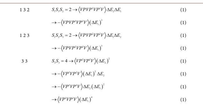
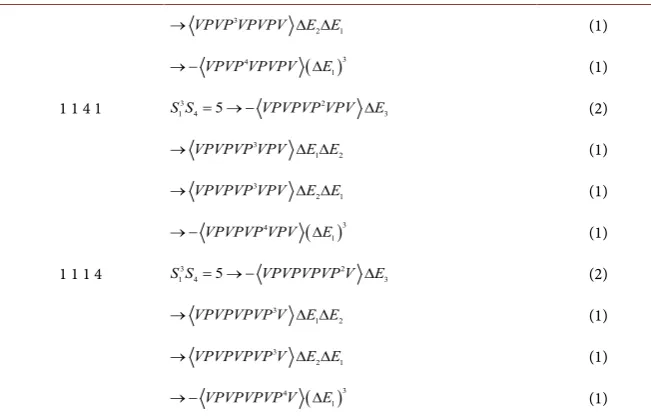
In a similar way the results for the perturbation terms belonging to N =7 and N=8_{are obtained; the terms are represented in}_{Tables 1-6}_.

9. Comparison of the Present Method with an Earlier

Recurrent Approach to the Perturbation Energy [34]

In [34] we presented a formalism which makes a recurrent calculation of the Schrödinger perturbation energy possible for an arbitrary order N. The me-thod—outlined in the present paper—is based on partitions of the number

1

(16)

[image:16.595.209.535.116.731.2]

Table 1. N=7. Perturbation terms based on the smaller size of partitions of the number 1 6

N− = . Total number of the perturbation terms in the Table:

( ) ( ) ( ) ( ) ( ) ( )

6 + 7 + 8 + 12 + 4 = 37 _.

1 1 1 1 1 1 6

1 1

S = → VPVPVPVPVPVPV ₍₁₎

2 1 1 1 1 4 2

2 1 1 1

S S = → −VP VPVPVPVPV ∆E ₍₁₎

1 2 1 1 1 4 2

2 1 1 1

S S = → −VPVP VPVPVPV ∆E ₍₁₎

1 1 2 1 1 4 2

2 1 1 1

S S = → −VPVPVP VPVPV ∆E ₍₁₎

1 1 1 2 1 4 2

2 1 1 1

S S = → −VPVPVPVP VPV ∆E ₍₁₎

1 1 1 1 2 4 2

2 1 1 1

S S = → −VPVPVPVPVP V ∆E ₍₁₎

2 2 1 1 2 2 2 2 ( )2

2 1 1 1

S S = → VP VP VPVPV ∆E ₍₁₎

2 1 2 1 2 2 2 2 ( )2

2 1 1 1

S S = → VP VPVP VPV ∆E ₍₁₎

2 1 1 2 2 2 2 2 ( )2

2 1 1 1

S S = → VP VPVPVP V ∆E ₍₁₎

1 2 2 1 2 2 2 2 ( )2

2 1 1 1

S S = → VPVP VP VPV ∆E ₍₁₎

1 2 1 2 2 2 2 2 ( )2

2 1 1 1

S S = → VPVP VPVP V ∆E ₍₁₎

1 1 2 2 2 2 2 2 ( )2

2 1 1 1

S S = → VPVPVP VP V ∆E ₍₁₎

2 2 2 3 2 2 2 ( )3

2 1

S = →1 −VP VP VP V ∆E (1)

3 1 1 1 3 2

3 1 2 2

S S = → −VP VPVPVPV ∆E (1)

( )2 3

1

VP VPVPVPV ∆E

→ ₍₁₎

1 3 1 1 3 2

3 1 2 2

S S = → −VPVP VPVPV ∆E ₍₁₎

( )2 3

1

VPVP VPVPV ∆E

→ ₍₁₎

1 1 3 1 3 2

1 3 2 2

S S = → −VPVPVP VPV ∆E ₍₁₎

( )2 3

1

VPVPVP VPV ∆E

→ ₍₁₎

1 1 1 3 3 2

1 3 2 2

S S = → −VPVPVPVP V ∆E ₍₁₎

( )2 3

1

VPVPVPVP V E

→ ∆ ₍₁₎

3 2 1 2 2

3 2 1 2 2 1

S S S = →VP VP VPV ∆E E∆ ₍₁₎

( )3 3 2

1

VP VP VPV ∆E

→ − ₍₁₎

3 1 2 2 2

3 1 2 2 2 1

S S S = →VP VPVP V ∆E E∆ ₍₁₎

( )3 3 2

1

VP VPVP V ∆E

→ − ₍₁₎

2 3 1 2 2

2 3 1 2 1 2

S S S = →VP VP VPV ∆E E∆ ₍₁₎

( )

3 2 3

1

VP VP VPV ∆E

→ − ₍₁₎

2 1 3 2 2

2 1 3 2 1 2

S S S = →VP VPVP V E E∆ ∆ ₍₁₎

( )3 3

1

VPVPVP V ∆E

(17)

DOI: 10.4236/wjm.2019.95009 129 World Journal of Mechanics Continued

1 3 2 2 2

1 3 2 2 2 1

S S S = →VPVP VP V ∆E E∆ ₍₁₎

( )3 3 2

1

VPVP VP V ∆E

→ − ₍₁₎

1 2 3 2 2

1 2 3 2 1 2

S S S = →VPVP VP V ∆E E∆ ₍₁₎

( )3 2 3

1

VPVP VP V ∆E

→ − ₍₁₎

3 3 2 2 ( )2

3 3 4 2

S S = → VP VP V ∆E ₍₁₎

( )2 3 2

1 2

VP VP V ∆E E

→− ∆ (1)

( )2 2 3

2 1

VP VP V ∆E ∆E

→ − (1)

( )4 3 3

1

VP VP V ∆E

[image:17.595.208.534.82.253.2]

→ ₍₁₎

Table 2. N=7. Perturbation terms based on the intermediate size of partitions of the number N− =1 6. Total number of the perturbation terms:

( ) ( ) ( ) ( ) ( ) ( )

5 + 5 + 5 + 14 + 14 = 53 .

4 1 1 2 2

4 1 5 3

S S = → −VP VPVPV ∆E ₍₂₎

3

1 2

VP VPVPV ∆ ∆E E

→ ₍₁₎

3

2 1

→ (1)

( )3 4

1

VP VPVPV ∆E

→ − ₍₁₎

1 4 1 2 2

1 4 5 3

S S = → −VPVP VPV ∆E ₍₂₎

3

1 2

VPVP VPV ∆ ∆E E

→ (1)

3

2 1

→ ₍₁₎

( )3 4

1

VPVP VPV ∆E

→ − ₍₁₎

1 1 4 2 2

1 4 5 3

S S = →−VPVPVP V ∆E ₍₂₎

3 1 2

VPVPVP V ∆ ∆E E

→ ₍₁₎

3 2 1

→ ₍₁₎

( )3 4

1

VPVPVP V ∆E

→ − ₍₁₎

4 2 2 2

4 2 5 3 1

S S = → VP VP V ∆E E∆ ₍₂₎

( )2 3 2

1 2

VP VP V ∆E E

→− ∆ ₍₁₎

3 2

1 2 1

VP VP V ∆ ∆ ∆E E E

→ − ₍₁₎

( )4 4 2

1

VP VP V ∆E

→ ₍₁₎

2 4 2 2

2 4 5 1 3

S S = → VP VP V ∆E E∆ ₍₂₎

2 3

1 2 3

VP VP V ∆ ∆ ∆E E E

→ − ₍₁₎

( )2 2 3

2 1

VP VP V ∆E ∆E

(18)

( )4 2 4

1

VP VP V ∆E

→ ₍₁₎

5 1 2

5 1 14 4

S S = → −VP VPV ∆E ₍₅₎

3

3 1

VP VPV ∆ ∆E E

→ ₍₂₎

( )2 3

2

VP VPV ∆E

→ ₍₁₎

3

1 3

→ ₍₂₎

( )2 4

1 2

VP VPV ∆E E

→− ∆ ₍₁₎

4

1 2 1

VP VPV ∆ ∆ ∆E E E

→ − ₍₁₎

( )2 4

2 1

VP VPV ∆E ∆E

→ − ₍₁₎

( )4 5

1

VP VPV ∆E

→ ₍₁₎

1 5 2

1 5 14 4

S S = →−VPVP V ∆E ₍₅₎

3 3 1

VPVP V ∆ ∆E E

→ ₍₂₎

( )2 3

2

VPVP V ∆E

→ ₍₁₎

3 1 3

→ ₍₂₎

( )2 4

1 2

VPVP V ∆E E

→− ∆ ₍₁₎

4

1 2 1

VPVP V ∆ ∆ ∆E E E

→ − ₍₁₎

( )2 4

2 1

VPVP V ∆E ∆E

→ − ₍₁₎

( )4 5

1

VPVP V ∆E

[image:18.595.207.538.526.736.2]

→ (1)

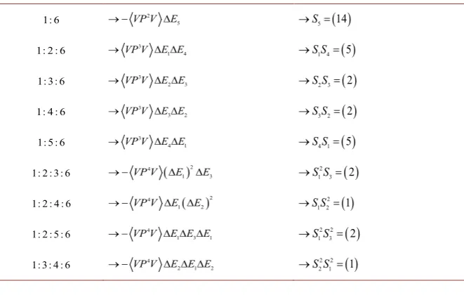
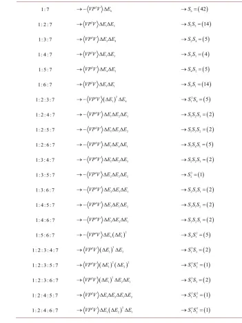
Table 3. N=7. The 42 energy perturbation terms belonging to partition 6=N−1. The time-point contractions applied in the Table are presented. The number in brackets at the end of each row indicates the number of the perturbation terms due to that row. Total number of terms in Tables 1-3:

( ) ( ) ( )

37 + 53 + 42 =132=S7.

1: 6 2

5

VP V E

→ − ∆ → =S₅

( )

14

1: 2 : 6 3 1 4

VP V E E∆ ∆

→ →S S_{1 4}=

( )

5

1: 3: 6 2

3 3

VP V E E∆ ∆

→ →S S2 3=

( )

2

1: 4 : 6 3

3 2

VP V E E∆ ∆

→ →S S3 2=

( )

2

1: 5 : 6 4

3 1

VP V E E∆ ∆

→ →S S_{4 1}=

( )

5

1: 2 : 3: 6 4 ( )2 1 3

VP V ∆E ∆E

→ − 2

( )

1 3 2

S S

→ =

1: 2 : 4 : 6 4 ( )2 1 2

VP V ∆E ∆E

→ − 2

( )

1 2 1

S S

→ =

1: 2 : 5: 6 4

1 3 1

VP V E E E

→− ∆ ∆ ∆ 2 2

( )

1 3 2

S S

→ =

1: 3: 4 : 6 4

2 1 2

VP V E E E

→− ∆ ∆ ∆ 2 2

( )

2 1 1

S S

(19)

1: 3: 5 : 6 4 ( )2 2 1

VP V ∆E ∆E

→ − 2 2

( )

2 1 1

S S

→ =

1: 4 : 5: 6 4 ( )2 3 1

VP V ∆E ∆E

→ − 2

( )

3 1 2

S S

→ =

1: 2 : 3: 4 : 6 ( 1)3 2 5

VP V E E

→ ∆ ∆ 3

( )

1 2 1

S S

→ =

1: 2 : 3: 5 : 6 5 ( )2 1 2 1

VP V ∆E ∆ ∆E E

→ 3

( )

1 2 1

S S

→ =

1: 2 : 4 : 5 : 6 5 ( )2 1 2 1

VP V E E∆ ∆E

→ ∆ 3

( )

1 2 1

S S

→ =

1: 3: 4 : 5 : 6 5 ( )3 2 1

VP V E ∆E

→ ∆ 3

( )

1 2 1

S S

→ =

1: 2 : 3: 4 : 5 : 6 6 ( )5 1

VP V ∆E

→ − 5

( )

1 1

S

[image:19.595.205.538.286.736.2]

→ =

Table 4. N=8. Perturbation terms based on the lower-size partitions of the number 1 7

N− = . Total number of the perturbation terms represented in Table 4:

( ) ( ) ( ) ( ) ( ) ( ) ( )

7 + 10 + 4 + 10 + 24 + 6 + 12 + ×4 5

( ) ( )

= 93 .

1 1 1 1 1 1 1 7

1 1

S = →VPVPVPVPVPVPVPV (1)

2 1 1 1 1 1 5 2

2 1 1 1

S S = → −VP VPVPVPVPVPV ∆E ₍₁₎

1 2 1 1 1 1 5 2

2 1 1 1

S S = → −VPVP VPVPVPVPV ∆E ₍₁₎

1 1 2 1 1 1 5 2

2 1 1 1

S S = → −VPVPVP VPVPVPV ∆E ₍₁₎

1 1 1 2 1 1 5 2

2 1 1 1

S S = → −VPVPVPVP VPVPV ∆E ₍₁₎

1 1 1 1 2 1 5 2

2 1 1 1

S S = →−VPVPVPVPVP VPV ∆E ₍₁₎

1 1 1 1 1 2 5 2

2 1 1 1

S S = → −VPVPVPVPVPVP V ∆E ₍₁₎

2 2 1 1 1 2 3 2 2 ( )2

2 1 1 1

S S = → VP VP VPVPVPV ∆E ₍₁₎

1 2 1 1 2 3 2 2 2 ( )2

1 2 1 1

S S = → VPVP VPVPVP V ∆E ₍₁₎

1 1 2 1 2 3 2 2 2 ( )2

1 2 1 1

S S = → VPVPVP VPVP V ∆E ₍₁₎

1 1 1 2 2 3 2 2 2 ( )2

1 2 1 1

S S = → VPVPVPVP VP V ∆E ₍₁₎

2 1 1 1 2 3 2 2 2 ( )2

1 2 1 1

S S = → VP VPVPVPVP V ∆E ₍₁₎

2 1 2 1 1 2 3 2 2 ( )2

2 1 1 1

S S = → VP VPVP VPVPV ∆E ₍₁₎

2 1 1 2 1 2 3 2 2 ( )2

2 1 1 1

S S = → VP VPVPVP VPV ∆E ₍₁₎

1 2 2 1 1 2 3 2 2 ( )2

2 1 1 1

S S = → VPVP VP VPVPV ∆E ₍₁₎

1 1 2 2 1 3 2 2 2 ( )2

1 2 1 1

S S = → VPVPVP VP VPV ∆E ₍₁₎

1 2 1 2 1 3 2 2 2 ( )2

1 2 1 1

S S = → VPVP VPVP VPV ∆E ₍₁₎

2 2 2 1 3 2 2 2 ( )3

2 1 1 1

S S = →−VP VP VP VPV ∆E ₍₁₎

2 2 1 2 3 2 2 2 ( )3

2 1 1 1

S S = → −VP VP VPVP V ∆E ₍₁₎

2 1 2 2 3 2 2 2 ( )3

2 1 1 1

(20)

1 2 2 2 3 2 2 2 ( )3

1 2 1 1

S S = →−VPVP VP VP V ∆E ₍₁₎

3 1 1 1 1 4 2

3 1 2 2

S S = → −VP VPVPVPVPV ∆E ₍₂₎

( )2 3

1

VP VPVPVPVPV ∆E

→

1 3 1 1 1 4 2

1 3 2 2

S S = → −VPVP VPVPVPV ∆E ₍₂₎

( )2 3

1

VPVP VPVPVPV ∆E

→

1 1 3 1 1 4 2

1 3 2 2

S S = → −VPVPVP VPVPV ∆E ₍₂₎

( )2 3

1

VPVPVP VPVPV ∆E

→

1 1 1 3 1 4 2

1 3 2 2

S S = → −VPVPVPVP VPV ∆E ₍₂₎

( )2 3

1

VPVPVPVP VPV ∆E

→

1 1 1 1 3 4 2

1 3 2 2

S S = → −VPVPVPVPVP V ∆E ₍₂₎

( )2 3

1

VPVPVPVPVP V ∆E

→

3 2 1 1 2 2 2

3 2 1 2 2 1

S S S = → VP VP VPVPV ∆ ∆E E ₍₂₎

( )3 3 2

1

VP VP VPVPV ∆E

→ −

1 3 2 1 2 2 2

1 3 2 2 2 1

S S S = → VPVP VP VPV ∆ ∆E E ₍₂₎

( )3 3 2

1

VPVP VP VPV ∆E

→ −

2 1 3 1 2 2 2

2 1 3 2 1 2

S S S = → VP VPVP VPV ∆ ∆E E ₍₂₎

( )3 2 3

1

VP VPVP VPV ∆E

→ −

3 1 2 1 2 2 2

3 1 2 2 2 1

S S S = → VP VPVP VPV ∆ ∆E E ₍₂₎

( )3 3 2

1

VP VPVP VPV ∆E

→ −

2 3 1 1 2 2 2

2 3 1 2 1 2

S S S = → VP VP VPVPV ∆ ∆E E ₍₂₎

( )3 2 3

1

VP VP VPVPV ∆E

→ −

1 2 3 1 2 2 2

1 2 3 2 1 2

S S S = → VPVP VP VPV ∆ ∆E E ₍₂₎

( )3 2 3

1

VPVP VP VPV ∆E

→ −

1 1 2 3 2 2 2

1 2 3 2 1 2

S S S = → VPVPVP VP V ∆ ∆E E (2)

( )3 2 3

1

VPVPVP VP V ∆E

→ −

1 1 3 2 2 2 2

1 3 2 2 2 1

S S S = → VPVPVP VP V ∆ ∆E E ₍₂₎

( )3 3 2

1

VPVPVP VP V ∆E

→ −

1 2 1 3 2 2 2

1 2 3 2 1 2

S S S = → VPVP VPVP V ∆ ∆E E ₍₂₎

( )3 2 3

1

VPVP VPVP V ∆E

(21)

1 3 1 2 2 2 2

1 3 2 2 1 2

S S S = → VPVP VPVP V ∆ ∆E E ₍₂₎

( )3 3 2

1

VPVP VPVP V ∆E

→ −

2 1 1 3 2 2 2

2 1 3 2 1 2

S S S = → VP VPVPVP V ∆ ∆E E ₍₂₎

( )3 2 3

1

VP VPVPVP V ∆E

→ −

3 1 1 2 2 2 2

3 1 2 2 2 1

S S S = → VP VPVPVP V ∆ ∆E E ₍₂₎

( )3 3 2

1

VP VPVPVP V ∆E

→ −

3 2 2 2 2 2 2 ( )2

3 2 2 2 1

S S = → −VP VP VP V ∆E ∆E (2)

( )4 3 2 2

1

VP VP VP V ∆E

→

2 3 2 2 2 2 2

2 3 2 1 2 1

S S = →−VP VP VP V ∆ ∆E E E∆ ₍₂₎

( )4 2 3 2

1

VP VP VP V ∆E

→

2 2 3 2 2 2 2 ( )2

2 3 2 1 2

S S = → −VP VP VP V ∆E ∆E ₍₂₎

( )4 2 2 3

1

VP VP VP V ∆E

→

3 3 1 2 2 2 ( )2

3 1 4 2

S S = →VP VP VPV ∆E ₍₄₎

( )2 3 2

1 2

VP VP VPV ∆E E

→− ∆

( )2 2 3

2 1

VP VP VPV ∆E ∆E

→ −

( )4 3 3

1

VP VP VPV ∆E

→

3 1 3 2 2 2 ( )2

3 1 4 2

S S = →VP VPVP V ∆E ₍₄₎

( )2 3 2

1 2

VP VPVP V ∆E E

− ∆

→

( )2 2 3

2 1

VP VPVP V ∆E ∆E

→ −

( )4 3 3

1

VP VPVP V ∆E

→

1 3 3 2 2 2 ( )2

1 3 4 2

S S = →VPVP VP V ∆E ₍₄₎

( )2 3 2

1 2

VPVP VP V ∆E E

− ∆

→

( )2 2 3

2 1

VPVP VP V ∆E ∆E

→ −

( )4 3 3

1

VPVP VP V ∆E

→

4 1 1 1 3 2

4 1 5 3

S S = → −VP VPVPVPV ∆E (2)

3

1 2

VP VPVPVPV ∆ ∆E E

→ ₍₁₎

3

2 1

VP VPVPVPV ∆ ∆E E

→ ₍₁₎

( )3 4

1

VP VPVPVPV ∆E

→ − ₍₁₎

1 4 1 1 3 2

1 4 5 3

S S = → −VPVP VPVPV ∆E ₍₂₎

3

1 2

VPVP VPVPV ∆ ∆E E

(22)

3

2 1

VPVP VPVPV ∆ ∆E E

→ ₍₁₎

( )3 4

1

VPVP VPVPV ∆E

→ − ₍₁₎

1 1 4 1 3 2

1 4 5 3

S S = → −VPVPVP VPV ∆E ₍₂₎

3

1 2

VPVPVP VPV ∆ ∆E E

→ (1)

3

2 1

VPVPVP VPV ∆ ∆E E

→ ₍₁₎

( )3 4

1

VPVPVP VPV ∆E

→ − ₍₁₎

1 1 1 4 3 2

1 4 5 3

S S = → −VPVPVPVP V ∆E ₍₂₎

3 1 2

VPVPVPVP V ∆ ∆E E

→ ₍₁₎

3 2 1

VPVPVPVP V ∆ ∆E E

→ ₍₁₎

( )3 4

1

VPVPVPVP V ∆E

[image:22.595.208.534.85.293.2]

→ − ₍₁₎

Table 5. N=8. Perturbation terms based on the higher-size partitions of the number 1 7

N− = . Total number of the perturbation terms:

( )

( ) (

)

6 5× + ×2 10 + ×2 14 + ×3 14 + ×2 42 = 204 .

4 2 1 2 2

4 2 1 5 3 1

S S S = →VP VP VPV ∆E E∆ ₍₂₎

( )2 3 2

2 1

VP VP VPV ∆E ∆E

→ − ₍₁₎

3 2

1 2 1

VP VP VPV ∆ ∆E E E

→− ∆ ₍₁₎

( )2 4 2

1

VP VP VPV ∆E

→ (1)

4 1 2 2 2

4 1 2 5 3 1

S S S = →VP VPVP V ∆E E∆ ₍₂₎

( )2 3 2

2 1

VP VPVP V ∆E ∆E

→ − ₍₁₎

3 2

1 2 1

VP VPVP V ∆ ∆E E E

→− ∆ (1)

( )4 4 2

1

VP VPVP V ∆E

→ ₍₁₎

2 4 1 2 2

2 4 1 5 1 3

S S S = →VP VP VPV ∆E E∆ ₍₂₎

2 3

1 2 1

VP VP VPV ∆ ∆E E E

→− ∆ ₍₁₎

( )2 2 3

1 2

VP VP VPV ∆E E

→− ∆ (1)

( )4 2 4

1

VP VP VPV ∆E

→ ₍₁₎

2 1 4 2 2

2 1 4 5 1 3

S S S = →VP VPVP V ∆E E∆ ₍₂₎

( )2 2 3

1 2

VP VPVP V ∆E E

− ∆

→ ₍₁₎

2 3

1 2 1

VP VPVP V ∆ ∆E E E

→− ∆ ₍₁₎

( )4 2 4

1

VP VPVP V ∆E

→ ₍₁₎

1 2 4 2 2

1 2 4 5 1 3

(23)

( )2 2 3

1 2

VPVP VP V ∆E E

− ∆

→ ₍₁₎

2 3

1 2 1

VPVP VP V ∆ ∆E E E

→− ∆ ₍₁₎

( )4 2 4

1

VPVP VP V ∆E

→ ₍₁₎

1 4 2 2 2

1 5 2 5 3 1

S S S = → VPVP VP V ∆E E∆ ₍₂₎

( )2 3 2

2 1

VPVP VP V ∆E ∆E

→ − ₍₁₎

3 2

1 2 1

VPVP VP V ∆ ∆E E E

→− ∆ (1)

( )4 4 2

1

VPVP VP V ∆E

→ (1)

4 3 2 2

4 3 5 2 10 3 2

S S = × = → VP VP V ∆E E∆ ₍₂₎

( )2 3 2

1 2

VP VP V ∆E ∆E

→ − ₍₁₎

3 2

2 1 2

VP VP V ∆ ∆ ∆E E E

→ − ₍₁₎

( )3 4 2

1 2

VP VP V ∆E ∆E

→ ₍₁₎

( )2 2 3

3 1

VP VP V ∆E ∆E

→ − ₍₁₎

( )2 3 3

2 1 1

VP VP V E E∆ ∆E

→ ∆ ₍₁₎

( )2 3 3

1 2 1

→ ∆ ₍₁₎

( )5 4 3

1

VP VP V ∆E

→ − ₍₁₎

3 4 2 2

3 4 2 5 10 2 3

S S = × = → VP VP V ∆E E∆ ₍₂₎

2 3

2 1 2

VP VP V ∆ ∆ ∆E E E

→ − ₍₁₎

2 3

2 2 1

VP VP V ∆ ∆ ∆E E E

→ − ₍₁₎

( )3 2 4

2 1

VP VP V ∆E ∆E

→ ₍₁₎

( )2 3 2

1 3

VP VP V ∆E E

→− ∆ ₍₂₎

( )2 3 3

1 1 2

VP VP V E ∆E E

→ ∆ ∆ ₍₁₎

( )2 3 3

1 2 1

→ ∆ ∆ ₍₁₎

( )5 3 4

1

VP VP V ∆E

→ − ₍₁₎

5 2 2 2

5 2 14 4 1

S S = → VP VP V ∆E E∆ ₍₅₎

( )2 3 2

3 1

VP VP V ∆E ∆E

→ − (2)

( )2 3 2

2 1

VP VP V ∆E E

→− ∆ ₍₁₎

( )2 3 2

3 1

VP VP V ∆E ∆E

→ − ₍₂₎

( )3 4 2

2 1

VP VP V ∆E ∆E

→ ₍₁₎

( )2 4 2

1 2 1

→ ∆ ₍₁₎

( )2 4 2

1 2 1

(24)

( )5 5 2

1

VP VP V ∆E

→ − ₍₁₎

2 5 2 2

2 5 14 1 4

S S = → VP VP V ∆E E∆ ₍₅₎

( )2 2 3

1 3

VP VP V ∆E E

→− ∆ ₍₂₎

( )

2 3 3

1 2

VP VP V ∆E ∆E

→ − ₍₁₎

2 3

1 3 1

VP VP V ∆ ∆ ∆E E E

→ − ₍₂₎

( )3 2 4

1 2

VP VP V ∆E ∆E

→ ₍₁₎

( )

2 4

1 2 1 2

→ ∆ ∆ ₍₁₎

( )2 2 4

1 2 1

→ ∆ ₍₁₎

( )5 2 5

1

VP VP V ∆E

→ − ₍₁₎

5 1 1 2 2

5 1 14 4

S S = → −VP VPVPV ∆E ₍₅₎

3

1 3

→ ₍₂₎

( )2 3

2

VP VPVPV ∆E

→ ₍₁₎

3

3 1

→ ₍₂₎

( )2 4

1 2

VP VPVPV ∆E E

→− ∆ ₍₁₎

4

1 2 1

VP VPVPV ∆ ∆E E E

→− ∆ ₍₁₎

( )2 4

2 1

VP VPVPV ∆E ∆E

→ − ₍₁₎

( )4 5

1

VP VPVPV ∆E

→ (1)

1 5 1 2 2

1 5 14 4

S S = → −VPVP VPV ∆E (5)

3

1 3

→ ₍₂₎

( )2 3

2

VPVP VPV ∆E

→ ₍₁₎

3

3 1

→ ₍₂₎

( )2 4

1 2

VPVP VPV ∆E E

→− ∆ ₍₁₎

4

1 2 1

VPVP VPV ∆ ∆E E E

→− ∆ ₍₁₎

( )2 4

2 1

VPVP VPV ∆E ∆E

→ − ₍₁₎

( )4 5

1

VPVP VPV ∆E

→ ₍₁₎

1 1 5 2 2

1 5 14 4

S S = → −VPVPVP V ∆E ₍₅₎

3 1 3

→ ₍₂₎

( )2 3

2

VPVPVP V ∆E

→ ₍₁₎

3 3 1

→ ₍₂₎

( )2 4

1 2

VPVPVP V ∆E E

− ∆

(25)

4

1 2 1

VPVPVP V ∆ ∆E E E

→− ∆ ₍₁₎

( )2 4

2 1

VPVPVP V ∆E ∆E

→ − ₍₁₎

( )4 5

1

VPVPVP V ∆E

→ ₍₁₎

6 1 2

6 1 42 5

S S = → −VP VPV ∆E ₍₁₄₎

3

4 1

→ ₍₅₎

3

3 2

→ (2)

3

2 3

→ (2)

3

1 4

→ ₍₅₎

( )2 4

3 1

VP VPV ∆E ∆E

→ − ₍₂₎

( )2 4

2 1

VP VPV ∆E E

→− ∆ ₍₁₎

( )2 4

1 3

VP VPV ∆E E

→− ∆ ₍₂₎

( )2 4

1 2

VP VPV ∆E ∆E

→ − ₍₁₎

( )2 4

1 2

VP VPV ∆E ∆E

→ − ₍₁₎

( )2 4

1 3

VP VPV ∆E E

→− ∆ ₍₂₎

( )3 5

2 1

VP VPV ∆E ∆E

→ ₍₁₎

( )3 5

2 1

VP VPV ∆E ∆E

→ ₍₁₎

( )3 5

1 2

VP VPV ∆E ∆E

→ ₍₁₎

( )3 5

1 2

VP VPV ∆E ∆E

→ ₍₁₎

( )5 6

1

VP VPV ∆E

→ − ₍₁₎

1 6 2

1 6 42 5

S S = →−VPVP V ∆E ₍₁₄₎

3 1 4

→ ₍₅₎

3

2 3

→ ₍₂₎

3

3 2

→ ₍₂₎

3 4 1

→ ₍₅₎

( )2 4

1 3

VPVP V ∆E E

→− ∆ (2)

( )2 4

1 2

VPVP V ∆E ∆E

→ − ₍₁₎

( )2 4

1 3

VPVP V ∆E E

→− ∆ ₍₂₎

( )2 4

2 1

VPVP V ∆E E

→− ∆ ₍₁₎

( )2 4

2 1

VPVP V ∆E E

→− ∆ ₍₁₎

( )2 4

3 1

VPVP V ∆E ∆E