(Guest Editors)
ExpandNet: A Deep Convolutional Neural Network for High
Dynamic Range Expansion from Low Dynamic Range Content
D. Marnerides1,2, T. Bashford-Rogers3, J. Hatchett2and K. Debattista2
1Warwick Centre for Predictive Modelling (WCPM), University of Warwick, UK 2WMG, University of Warwick, UK
3Department of Computer Science and Creative Technologies, University of the West of England, UK
Abstract
High dynamic range (HDR) imaging provides the capability of handling real world lighting as opposed to the traditional low dynamic range (LDR) which struggles to accurately represent images with higher dynamic range. However, most imaging content is still available only in LDR. This paper presents a method for generating HDR content from LDR content based on deep Convolutional Neural Networks (CNNs) termed ExpandNet. ExpandNet accepts LDR images as input and generates images with an expanded range in an end-to-end fashion. The model attempts to reconstruct missing information that was lost from the original signal due to quantization, clipping, tone mapping or gamma correction. The added information is reconstructed from learned features, as the network is trained in a supervised fashion using a dataset of HDR images. The approach is fully automatic and data driven; it does not require any heuristics or human expertise. ExpandNet uses a multiscale architecture which avoids the use of upsampling layers to improve image quality. The method performs well compared to expansion/inverse tone mapping operators quantitatively on multiple metrics, even for badly exposed inputs.
CCS Concepts
•Computing methodologies→Neural networks; Image processing;
1. Introduction
High dynamic range (HDR) imaging provides the capability to cap-ture, manipulate and display real-world lighting, unlike traditional, low dynamic range (LDR) imaging. HDR has found many appli-cations in photography, physically-based rendering, gaming, films, medical and industrial imaging and recent displays support HDR content [SHS∗04,MdPVA16]. While HDR imaging has seen many advances, LDR remains the status quo, and the majority of both current and legacy content is predominantly LDR. In order to gain an improved viewing experience [AFR∗07], or to use this content in future HDR pipelines, LDR content needs to be converted to HDR.
A number of methods which can retarget LDR to HDR content have been presented [BADC17]. These methods make it possible to utilise and manipulate the vast amounts of LDR content within HDR pipelines and visualise them on HDR displays. However, such methods are primarily model-driven, use various parameters which make them difficult to use by non-experts, and are not suitable for all types of content.
Recent machine learning advances for applications in image pro-cessing provide data driven solutions for imaging problems, by-passing reliance on human expertise and heuristics. CNNs are the current de-facto approach used for many imaging tasks, due to their
high learning capacity as well as their architectural qualities which make them highly suitable for image processing [Sch14]. The net-works allow for abstract representations to be acquired directly from data, surpassing simplistic pixelwise processing. This acqui-sition of abstractness is especially strong when the networks are of sufficient depth [HZRS15]. This paper presents a method for HDR expansion based on deep Convolutional Neural Networks (CNNs).
In this work, a novel multiscale CNN architecture, called Ex-pandNet, is presented. On a local scale, one branch of the net-work learns how to maintain and expand high frequency detail, while a dilation branch learns information on larger pixel neigh-bourhoods. A final third branch provides overall information by learning the global context of the input. The architecture is de-signed to avoid upsampling of downsampled features, in an attempt to reduce blocking and/or haloing artefacts that may arise from more straightforward approaches, for example autoencoder archi-tectures [Ben09]. Results demonstrate an improvement in quality over all other previous approaches that were tested, including some other CNN architectures.
In summary, the primary contributions of this work are:
• Results which are competitive with the other approaches tested, including other CNN architectures applied to single exposure LDR to HDR.
• Data augmentation for limited HDR content via different expo-sure and position selection to obtain more LDR-HDR training pairs.
• A comprehensive quantitative comparison of LDR to HDR ex-pansion methods.
2. Related Work
A number of methods to expand LDR to HDR have been presented in the literature. Furthermore, deep learning methods have been used for similar problems in the past. The following subsections discuss these topics.
2.1. LDR to HDR
Expansion operators (EOs), also known as inverse or reverse tone mapping operators, attempt to generate HDR content from LDR content. EOs can generally be expressed as:
Le= f(Ld),wheref:[0,255]→R+ (1)
whereLecorresponds to the expanded HDR content,Ldto the LDR
input andf(·)is the EO. In this contextf(·)could be considered as an ill-posed function. However, a variety of methods have emerged that attempt to tackle this issue. The majority of EOs can be broadly divided into two categories: global and local methods [BADC17].
The global methods use a straightforward function to expand the content equally across all pixels. One of the first of such meth-ods was the technique presented by Landis [Lan02] which expands content based on power functions. A straightforward method that uses a linear transformation combined with gamma correction was presented by Akyüz et al. [AFR∗07] and evaluated using a subjec-tive experiment. Masia et al. [MAF∗09,MSG17] also presented a global method which expands the content based on image attributes defined by an image key.
Local methods typically expand LDR content to HDR through the use of an analytical function combined with an expand map. The inverse tone mapping method [BLDC06] initially expands the content using an inverted photographic tone reproduction tone mapper [RSSF02], although this could be applied to other tone mappers that are invertible. An expand map is generated by select-ing a constellation of bright points and expandselect-ing them via density estimation. This is subsequently used in conjunction with the in-verse tone mapping equation to map LDR values to HDR values to avoid quantization errors that would arise via inverse tone mapping only. Rempel et al. [RTS∗07] also used an expand map, however this was computed through the use of a Gaussian filter in conjunc-tion with an edge-stopping funcconjunc-tion to maintain contrast. Kovaleski and Oliviera [KO14] extended the work of Rempel et al. via the use of a cross bilateral filter. Subsequently, Huo et al. [HYDB14] further extended this work to remove the thresholding used by Ko-valeski and Oliviera.
Other methods include inpainting as used by Wang et
al. [WWZ∗07] which is partially user-based, and classification based methods such as by Meylan et al. [MDS06] and Didyk et al. [DMHS08], which operate on different parts of the image by classifying these parts accordingly.
Banterle et al. [BDA∗09] provide a broader view of these meth-ods. With most of the above, the added information is derived from heuristics that may produce sufficient results for well behaved in-puts, but are not data driven. Most importantly, most existing EOs find it difficult to handle under/over-exposed LDR content.
2.2. Deep Learning for Image Processing
Deep learning has been extensively used for image processing problems recently. In image-to-image translation [IZZE16b] the authors present a method based on Generative Adversarial Net-works [GPAM∗14] and the U-Net [RFB15] architecture that trans-forms images from one domain to another (e.g. maps to satel-lite). Many approaches have also been developed for other kinds of ill-posed or inverse problems, including image super-resolution and upsampling [DLHT16,KLL15,YKK17] as well as inpaint-ing/hallucination of missing information [ISSI17]. Automatic col-orization [ISSI16] converts grey scale to color images using a CNN which uses two routes of computation, fusing local and global con-text for improved image quality.
In visualization, graphics and HDR imaging, neural net-works have been used for predicting sky illumination for ren-dering [SBRCD17,HGSH∗17], denoising Monte Carlo render-ings [KBS15,CKS∗17,BVM∗17], predicting HDR environment maps [ZL17a], reducing artefacts such as ghosting when fusing multiple LDR exposures to create HDR content [KR17] and for tone mapping [HDQ17].
Concurrently to this work, two other deep learning approaches that expand LDR content to HDR have been developed. Eilertsen et al. [EKD∗17], use a U-Net like architecture to predict values for saturated areas of badly exposed content, whereas non-saturated areas are linearised by applying an inverse camera response curve. Endo et al. [EKM17] use a modified U-Net architecture that pre-dicts multiple exposures from a single exposure which are then used to generate an HDR image using standard merging algorithms.
The first method does not suffer greatly from artefacts pro-duced from upsampling that are common with U-Net and simi-lar architectures [ODO16] since only areas of badly exposed con-tent are expanded by the network. In the latter, the authors men-tion the appearance of tiling artefacts in some cases. There are other examples in literature when fully converged U-Net like net-works exhibit artefacts, for example in image-to-image translation tasks [IZZE16a], or semantic segmentation [ZL17b]. Our approach differs from these methods methods as it presents a dedicated ar-chitecture for and end-to-end image expansion, without using up-sampling.
3. ExpandNet
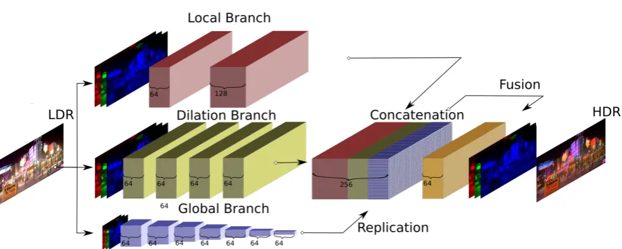
Figure 1: ExpandNet architecture. The LDR input is propagated through the the local and dilation branches, while a resized input (256×256) is propagated through the global branch. The output of the global branch is superposed over each pixel of the outputs of the other two branches. The resulting features are fused using 1×1 convolutions to form the last feature layer which then gives an RGB HDR prediction.
branch architecture. Figure1presents an overview of the architec-ture. The three branches of computation are a local, a dilation and a global one. Each branch is itself a CNN that accepts an RGB LDR image as input. Each one of the three branches is responsible for a particular aspect, with the local branch handling local detail, the dilation branch for medium level detail, and a global branch accounting for higher level image-wide features.
The local and dilation branches avoid any use of downsampling and upsampling, which is a common approach in the design of CNNs, and the global branch only downsamples. In image process-ing CNNs it is common to downsample the width and height of the input image, while expanding the channel dimension. This forms a set of more abstract features after a few layers of downsampling. The features are then upsampled to the original dimensions, for ex-ample in autoencoders. As also mentioned in the previous section, it is argued [ODO16] that upsampling, especially the frequently used deconvolutional layers [SCT∗16], cause checkerboard arte-facts. Furthermore, upsampling may cause unwanted information bleeding in areas where context is missing, for example large over-exposed areas. Figure11and Figure12(b) and (c), discussed fur-ther in Section5, provide examples where such artefacts can arise in upsampling networks, seen as blocking in (b) due to deconvo-lutions, and banding in (c) due to nearest-neighbour upsampling. ExpandNet avoids the use of upsampling layers to reduce such arte-facts and improves the quality of the predicted HDR images.
The outputs of the three branches are fused and further processed by a small final convolutional layer that produces the predicted HDR image. The input LDR and the predicted HDR are both in the[0,1]range.
The following subsection briefly introduces CNNs, followed by a detailed overview of the three branches of the ExpandNet archi-tecture, including design characteristics for feature fusion, activa-tion funcactiva-tions and the loss funcactiva-tion used for optimizaactiva-tion.
3.1. Convolutional Neural Networks
A feed-forward neural network (NN) is a function composed of multiple layers of non-linear transformations. Given an input vec-torx, a network ofM layers (with no skip connections) can be expressed as follows:
fNN(x) = (lM◦lM−1◦ · · · ◦l2◦l1)(x) (2) whereliis theithhidden layer of the network and◦is the
compo-sition operator. Each layer accepts the output of the previous layer, oi−1, and applies a linear map followed by a non-linear transfor-mation:
oi=li(oi−1) =α(Wioi−1) (3) whereWiis a matrix of learnable parameters (weights),oN is the
network output ando0 =x. α(z)is a non-linear (scalar) activa-tion funcactiva-tion, applied to each value of the resulting vector inde-pendently. A learnable bias term exists in the linear map as well, but is folded inWi(andx) for ease of notation.
A convolutional layer, ci, uses sparse parameter matrices with
repeated values. The sparsity and repetition structure is such, so that the linear product can be expressed as a convolution,∗, between a learnable parameter filter ˜wand the input to the layer.
ci(oi−1) =α(w˜i∗oi−1) (4)
This formulation is analogous for higher dimensions. In the scope of this work, images are three dimensional objects (width×
height×channels / features), thus the parameter matrices become four-dimensional tensors. For image processing CNNs, the convo-lutions are usually only in the width and height dimensions, while the third dimension is fully connected (dense tensor dimension).
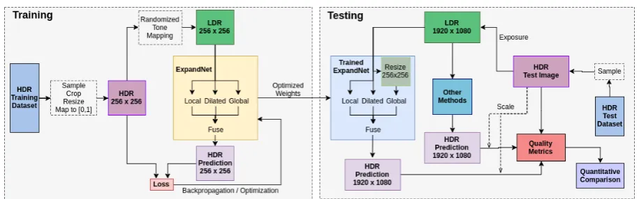
Figure 2: General overview of the workflow. (left) The training dataset is sampled and preprocessed on-the-fly to form 256×256 resolution input-output pairs, which are then used to optimize the network weights. (right) For testing, the images are full-HD (1,920×1,080). The luminance of the predictions of all methods is scaled either to match the original HDR image (scene-referred) or that of a 1,000cd/m2 display (display-referred).
3.2. Branches
The three branches play different roles in expanding the dynamic range of the input LDR. The global branch seeks to reduce the di-mensionality of the input and capture abstract features. It has a suf-ficiently large receptive field that covers the whole image. It accepts the entire LDR image as input, re-sized to 256×256, and eventu-ally downsamples it to 1×1 over a total of seven layers. Each layer has 64 feature maps and uses stride 2 convolutions which consecu-tively downsample the spatial dimensions by a factor of 2. All the global branch layers use a convolutional kernel of size 3×3, with padding 1 except the last layer which uses a 4×4 kernel with no padding, essentially densely connecting the previous layer, which consists of 4×4 features, with the last layer, creating a vector of 1×1 features.
The other two branches provide localized processing without downsampling that captures higher frequencies and neighbouring features. The local branch has a receptive field of 5×5 pixels and consists of two layers with 3×3 convolutions of stride 1 and padding 1, with 64 and 128 feature maps respectively. The small re-ceptive field of the local branch provides learning at the pixel level, preserving high frequency detail.
The dilation branch has a wider receptive field of 17×17 pix-els and uses dilated convolutions [YK15] of dilation size 2, kernel 3×3, stride 1, and padding 2. Dilated convolutions are large, sparse convolutional kernels, used to quickly increase the receptive field of CNNs. A total of four dilation layers are used each with 64 features. With an increased receptive field, the dilation network captures lo-cal features with medium range frequencies otherwise missed by the other two branches whose focus is on the two extremes of the frequency spectrum.
The effects of each individual branch are presented in Figure3. Masking the input to an individual branch causes the output ap-pearance to change, depending on which branch was masked, high-lighting its role. The local branch produces high frequency fea-tures, while the dilation branch adds medium range frequencies. The global branch changes the overall appearance of the output by
adding low frequencies and adjusting the overall sharpness of the image. Results, shown in Section5.3, further help to illustrate the advantages posed by the three distinct branches.
3.3. Fusion
The outputs of the three branches are merged in a manner similar to the fusion layer by Iizuka et al. [ISSI16]. The local and dilation outputs, which have the same height and width as the input, are concatenated along the feature map dimension. The output of the global network is a vector of 64 features which is replicated along the width and height dimensions to match the dimensions of the other two outputs. The replication superposes the vector over each pixel of the predictions of the other two branches. It is then concate-nated with the rest of the outputs along the feature map dimension resulting in a total of 256 features. The concatenation is followed by a convolution of kernel size 1×1 which fuses the global feature vector with each individual pixel of the local and dilated features, thus combining context from multiple scales. The output of the fu-sion layer is further processed by a final convolutional layer with 3×3 kernels, stride 1 and padding 1.
3.4. Activations
All the layers, besides the output layer, use the Scaled Exponential Linear Unit (SELU) activation function [KUMH17], a variation of the Exponential Linear Unit (ELU).
SELU(z) =β (
z ifz>0
αez−α ifz≤0 (5)
(a) Local + Dilated + Global (b) Local + Global (c) Dilated + Global
[image:5.595.78.534.74.283.2](d) Local + Dilated (e) Local (f) Dilated
Figure 3: Illustration of the contribution of each of the three branches of ExpandNet. These images were obtained by masking one or more branches with zero inputs. The bottom row is produced with the global branch masked. This causes the overall appearance of the images to be darker and sharper, since there are low frequencies missing. The middle column masks the dilation branch, resulting in sharp high-frequency images. The right column masks the local branch which causes most of the fine details to be lost.
Table 1: Parameters used for tone mapping. All images are fol-lowed by a gamma correction curve withγ∈[1.8,2.2]. Values given within ranges are sampled from a uniform distribution.
TMO Parameters
Photoreceptor
Intensity:[−1.0,1.0] Light adaptation:[0.8,1.0] Color adaptation:[0.0,0.2]
ALM Saturation: 1.0, Bias:[0.7,0.9]
Display Adaptive Saturation: 1.0, Scale:[0.65,0.85]
Bilateral Saturation: 1.0, Contrast:[3,5] σspace: 8,σcolor: 4
Exposure Percentile:[0,15]to[85,100]
(ReLU). ReLUs alleviate the vanishing/exploding gradient prob-lem [KSH17] that was frequent with the traditional Sigmoid acti-vations (when stacked), while ELUs improve the sparse activation problem of the ReLUs by providing negative activation values.
The final layer of the network uses a Sigmoid activation,
σ(z) = 1
1+e−z (6)
which maps the output to the[0,1]range.
3.5. Loss function
The Loss function,L, used for optimizing the network is theL1 distance between the predicted image, ˜I, and real HDR image,I, from the dataset. TheL1distance is chosen for this problem since
the more frequently usedL2 distance was found to cause blurry results for images [MCL15]. An additional cosine similarity term is added to ensure color correctness of the RGB vectors of each pixel.
Li=kI˜i−Iik1+λ 1−1
K
K
∑
j=i
˜ Iij·Iij
kI˜j ik2kIijk2
!
(7)
whereLi is the loss contribution of theith image of the dataset,
λis a constant factor that adjusts the contribution of the cosine similarity term,Iijis thejthRGB pixel vector of imageIiandKis
the total number of pixels of the image.
Cosine similarity measures how close two vectors are by com-paring the angle between them, not taking magnitude into account. For the context of this work, it ensures that each pixel points in the same direction of the three dimensional RGB space. It provides im-proved color stability, especially for low luminance values, which are frequent in HDR images, since slight variations in any of the RGB components of these low values do not contribute much to theL1loss, but they may however cause noticeable color shifts.
3.6. Training
4. Training and Implementation
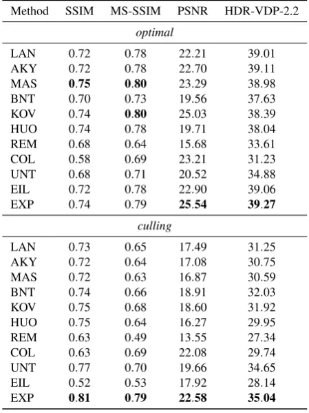
[image:5.595.67.277.403.530.2]Table 2: Average values of the four metrics for all methods for scene-referred scaling. Bold values indicate the best value.
Method SSIM MS-SSIM PSNR HDR-VDP-2.2
optimal
LAN 0.72 0.78 22.21 39.01 AKY 0.72 0.78 22.70 39.11 MAS 0.75 0.80 23.29 38.98 BNT 0.70 0.73 19.56 37.63 KOV 0.74 0.80 25.03 38.39 HUO 0.74 0.78 19.71 38.04 REM 0.68 0.64 15.68 33.61 COL 0.58 0.69 23.21 31.23 UNT 0.68 0.71 20.52 34.88 EIL 0.72 0.78 22.90 39.06
EXP 0.74 0.79 25.54 39.27
culling
LAN 0.73 0.65 17.49 31.25 AKY 0.72 0.64 17.08 30.75 MAS 0.72 0.63 16.87 30.59 BNT 0.74 0.66 18.91 32.03 KOV 0.75 0.68 18.60 31.92 HUO 0.75 0.64 16.27 29.95 REM 0.63 0.49 13.55 27.34 COL 0.63 0.69 22.08 29.74 UNT 0.77 0.70 19.66 34.65 EIL 0.52 0.53 17.92 28.14
EXP 0.81 0.79 22.58 35.04
4.1. Dataset
A dataset of HDR images was created consisting of 1,013 training images and 50 test images, with resolutions ranging from 800×800 up to 4,916×3,273. The images were collected from various sources, including in-house images, frames from HDR videos and the web. Only 100 of the images contained calibrated luminance values, sourced from the Fairchild database [Fai07]. All the images contained linear RGB values. The 50 test images used for evalua-tion in Secevalua-tion5were selected randomly from the Fairchild images with calibrated absolute luminance. LDR content for training was generated on-the-fly, directly from the dataset, and was augmented in a number of ways as outlined below.
At every epoch each HDR image from the training set is used as input in the network once after preprocessing. Preprocessing con-sists of randomly selecting a position for a sub image, cropping, and having its dynamic range reduced using one of a set of operators. The randomness entails that at every epoch a different LDR-HDR pair is generated from a single HDR image in the training set.
[image:6.595.59.284.114.414.2]Initially, the HDR image has its cropping position selected. The position is drawn from a spatial Gaussian distribution such that the most frequently selected regions are towards the center of the im-age. The crop size is drawn from an exponential distribution such that smaller crops are more frequent than larger ones, with a min-imum crop size of 384×384. Randomly cropping the images is a
Table 3: Average values of the four metrics for all methods for display-referred scaling. Bold values indicate the best value.
Method SSIM MS-SSIM PSNR HDR-VDP-2.2
optimal
LAN 0.76 0.80 19.89 41.01 AKY 0.76 0.80 20.37 40.89 MAS 0.79 0.82 21.03 40.83 BNT 0.74 0.75 17.22 39.99 KOV 0.80 0.83 23.01 40.00 HUO 0.77 0.77 17.83 38.58 REM 0.66 0.59 14.60 33.74 COL 0.63 0.71 21.00 31.41 UNT 0.72 0.73 18.23 35.68 EIL 0.77 0.80 20.66 41.01 EXP 0.79 0.82 23.43 40.81
culling
LAN 0.31 0.17 9.12 18.01 AKY 0.74 0.66 15.00 31.39 MAS 0.73 0.64 14.77 31.11 BNT 0.36 0.27 9.61 24.51 KOV 0.77 0.69 16.54 31.78 HUO 0.74 0.64 14.85 30.57 REM 0.59 0.46 12.81 27.96 COL 0.66 0.70 19.99 30.26 UNT 0.78 0.69 17.02 35.27 EIL 0.54 0.55 15.96 27.58
EXP 0.83 0.79 19.93 36.21
standard technique for data augmentation. Choosing the crop size at random adds another layer of augmentation, since the likelihood of picking the same crop is reduced, but it also aids in how well the model generalizes since it provides different sized content for similar scenes.
The cropped image is resized to 256×256 and linearly mapped to the[0,1]range to create the output. Since only a small fraction of the dataset images contain absolute luminance values, the network was trained to predict relative luminance values in the[0,1]range.
REMHUO BNT UNT LAN AKY EIL MAS COL KOL EXP Method 5 10 15 20 25 30 35 40 pu -P SN R
COL REM UNT BNT HUO AKY LAN EIL EXP KOL MAS Method 0.3 0.4 0.5 0.6 0.7 0.8 0.9 1.0 pu -S SI M
REM COL UNT BNT HUO EXP KOL AKY MAS EIL LAN Method 0.4 0.5 0.6 0.7 0.8 0.9 1.0 pu -M S-SS IM
[image:7.595.320.549.80.257.2]COL REM UNT BNT EXP HUO LAN AKY EIL MAS KOL Method 10 20 30 40 50 60 H DR -V DP -2
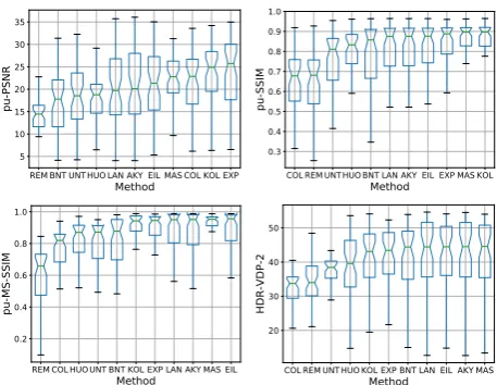
Figure 4: Box plots for scene-referred HDR obtained from LDR via optimalexposure.
REMHUOMAS AKY LAN EIL KOL BNT UNT COL EXP Method 5 10 15 20 25 30 35 pu -P SN R
REM COL MAS AKY HUO KOL EIL LAN BNT UNT EXP Method 0.2 0.3 0.4 0.5 0.6 0.7 0.8 0.9 pu -S SI M
REMHUOMAS AKY BNT KOL EIL LAN COL UNT EXP Method 0.2 0.3 0.4 0.5 0.6 0.7 0.8 0.9 pu -M S-SS IM
[image:7.595.57.287.82.257.2]REMHUO COL AKY MAS KOL BNT LAN EIL EXP UNT Method 10 15 20 25 30 35 40 45 H DR -V DP -2
Figure 5: Box plots for scene-referred HDR obtained from LDR via culling.
section only use single exposures for generating HDR; the TMOs are just used for data augmentation during training.
4.2. Optimization
The network parameters are optimized to minimize the loss given in Equation7, withλ=5, using mini-batch gradient descent and the backpropagation algorithm [RHW86]. The Adam optimizer was used [KB14], with an initial learning rate of 7e−5 and a batch size of 12. After the first 10,000 epochs, the learning rate was re-duced by a factor of 0.8 whenever the loss reached a plateau, until the learning rate reached values less than 1e−7 for a total of 1,600 epochs extra.L2regularization (weight decay) was used to reduce the chance of overfitting. All experiments were implemented using the PyTorch library [pyt]. Training time took a total of 130 hours on an Nvidia P100.
REM BNT UNT HUO LAN AKY EIL MAS COL KOL EXP Method 5 10 15 20 25 30 35 pu -P SN R
COL REM UNT HUO BNT LAN AKY EIL EXP MAS KOL Method 0.3 0.4 0.5 0.6 0.7 0.8 0.9 1.0 pu -S SI M
REM COL HUO UNT BNT KOL EXP LAN AKY MAS EIL Method 0.2 0.4 0.6 0.8 1.0 pu -M S-SS IM
[image:7.595.320.550.305.479.2]COL REM UNT HUO KOL EXP BNT LAN EIL AKY MAS Method 20 30 40 50 H DR -V DP -2
Figure 6: Box plots for display-referred HDR obtained from LDR viaoptimalexposure.
BNT LAN REM MASHUO AKY KOL UNT EIL COL EXP Method 5 10 15 20 25 30 pu -P SN R
BNT LAN EIL REM COL HUOMAS KOL AKY UNT EXP Method 0.2 0.4 0.6 0.8 1.0 pu -S SI M
LAN BNT REM EIL HUOMAS AKY KOL COL UNT EXP Method 0.0 0.2 0.4 0.6 0.8 1.0 pu -M S-SS IM
LAN BNT REM EIL COL HUO AKY MAS KOL UNT EXP Method 15 20 25 30 35 40 45 H DR -V DP -2
Figure 7: Box plots for display-referred HDR obtained from LDR viaculling.
5. Results
This section presents an evaluation of ExpandNet compared to other EOs and deep learning architectures. Figure2(right) shows an overview of the evaluation method.
5.1. Quantitative
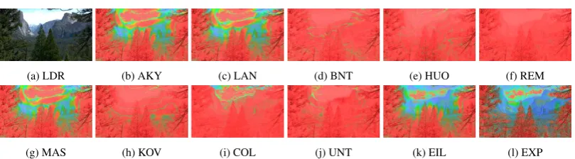
[image:7.595.58.287.307.481.2](a) LDR (b) AKY (c) LAN (d) BNT (e) HUO (f) REM
[image:8.595.90.506.70.189.2](g) MAS (h) KOV (i) COL (j) UNT (k) EIL (l) EXP
Figure 8: HDR-VDP-2.2 visibility probability maps for predictions of (culling) M3 Middle Pond using all methods. Blue indicates imper-ceptible differences, red indicates perimper-ceptible differences.
(a) LDR (b) AKY (c) LAN (d) BNT (e) HUO (f) REM
[image:8.595.103.507.230.339.2](g) MAS (h) KOV (i) COL (j) UNT (k) EIL (l) EXP
Figure 9: HDR-VDP-2.2 visibility probability maps for predictions of (culling) Devils Bathtub using all methods. Blue indicates impercep-tible differences, red indicates percepimpercep-tible differences.
The ExpandNet architecture is compared against seven other previous methods for dynamic range expansion/inverse tone map-ping. The chosen methods were the methods of: Landis [Lan02] (LAN), Banterle et al. [BLDC06] (BNT), Akyüz et al. [AFR∗07] (AKY), Rempel et al. [RTS∗07] (REM), Masia et al. [MAF∗09] (MAS), Kovaleski and Oliveira [KO14] (KOV) and Huo et al. [HYDB14] (HUO). The Matlab implementations from the HDR toolbox [BADC17] were used to obtain these results.
Four CNN architectures are compared, including the proposed ExpandNet method (EXP). Two other network architectures that have been used for similar problems have been adopted and trained in the same way as EXP. The first network is based on U-Net [RFB15] (UNT), an architecture that has shown strong results with image translation tasks between domains. The second network is an architecture first used for colorization [ISSI16] (COL), which uses two branches and a fusion layer similar to the one used for ExpandNet. These three are implemented using the same pyTorch framework and trained on the same training dataset. The recent network architecture used for LDR to HDR conversion [EKD∗17] (EIL) is also included. The predictions from this method were cre-ated using the trained network which was made available online by the authors, applied on the same test dataset used for all the other methods.
The inputs to the methods are single exposure LDR images of the 50 full HD (1920×1080) images in the HDR test dataset. The single exposures are obtained using two methods. The first method (optimal) finds the optimal/automatic exposure [DBRS∗15] using the HDR image histogram, resulting in minimal clipping at the two
ends of the luminance range. The second method (culling) simply clips the top and bottom 10% of the values of the images, resulting in more information loss and distortion of the input LDR. The re-sulting test LDR input images are saved with JPEG encoding before testing. When compared to the 10thpercentile loss for the images generated usingculling, on average, the number of pixels over the test dataset that are over-exposed when usingoptimalis 3.89% and the number of pixels under-exposed is 0.35%.
The outputs of the methods are in the[0,1]range, predicting rel-ative luminance. The scaling permits evaluation for scene-referred and display-referred output. Hence, the predicted HDR images are scaled to match the original HDR content (scene-referred) and a 1,000cd/m2 display (display-referred), which represents current commercial HDR display technology. The scaling is done to match the 0.1 and 99.9 percentiles of the predictions with the correspond-ing percentiles of the HDR test images. Furthermore, scalcorrespond-ing is use-ful as the PU-encoded HDR metrics are dependent on absolute lu-minance values incd/m2. By scaling the prediction outputs, the PU-encoded metrics can be used to quantify the ability of the net-work to reconstruct the original signal.
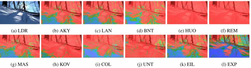
(a) LDR (b) AKY (c) LAN (d) BNT (e) HUO (f) REM
[image:9.595.102.507.76.188.2](g) MAS (h) KOV (i) COL (j) UNT (k) EIL (l) EXP
Figure 10: HDR-VDP-2.2 visibility probability maps for predictions of (culling) Tunnel View using all methods. Blue indicates imperceptible differences, red indicates perceptible differences.
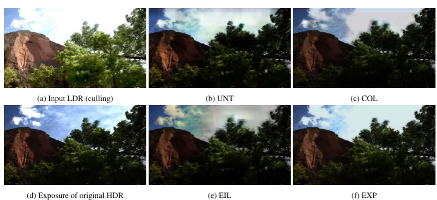
(a) Input LDR (culling) (b) UNT (c) COL
(d) Exposure of original HDR (e) EIL (f) EXP
Figure 11: (a) LDR input image created using culling from the Balanced Rock HDR image. (d) Low exposure of the original HDR image. (b,c,e,f) Low exposure slices of the predictions from methods that use CNN architectures showing artefacts.
amongst all the methods, a significance is found for all tests (at p < 0.001) using Friedman’s test. Pairwise comparisons ranked EXP in the top group, consisting of the group of methods that cannot be significantly differentiated, in 13 of the 16 results (these consist of all four metrics for bothoptimalandcullingand for both scene-referred and display scene-referred). The conditions where EXP was not in the top group were: pu-SSIM (in the cases of scene-referred and display-referred) and pu-MMSIM (for scene-referred only); in all three cases this occurred for theoptimalcondition.
As can be seen in the overall, EXP performs reasonably well. In particular for thecullingcase when a significant number of pixels are over or under-exposed EXP appears to reproduce HDR better than the other methods. Foroptimal, EIL performs very well also, and this is expected as in such cases the number of pixels that are required to be predicted from the CNN are smaller. Similarly, the non deep learning based expansion methods such as MAS perform well especially for SSIM which quantifies structural similarity.
5.2. Visual Inspection
This section presents some qualitative aspects of the results. HDR-VDP-2.2 visibility probability maps for all the methods are
pre-sented, as well as images from the CNN predictions exhibiting ef-fects such as hallucination, blocking and information bleeding.
Figure8, Figure9and Figure10show the HDR-VDP-2.2 prob-ability maps for the predictions of all the methods from the test set. The HDRs are predicted fromcullingLDRs with scene-referred scaling. The HDR-VDP-2.2 visibility probability map describes how likely it is for a difference to be noticed by the average ob-server, at each pixel. Red values indicate high probability, while blue values indicate low probability. Results show EXP performs better than most other methods for these scenes. EIL also performs well, particularly for the challenging scenario in Figure10.
[image:9.595.97.508.230.418.2](a) Input LDR (culling) (b) UNT (c) COL
(d) Exposure of original HDR (e) EIL (f) EXP
Figure 12: (a) LDR input image created using culling from The Grotto HDR image. (d) Low exposure of the original HDR image. (b,c,e,f) Low exposure slices of the predictions from methods that use CNN architectures showing artefacts.
[image:10.595.86.518.74.272.2]exposure (scaling and clipping at 255) only have their B channel saturated (e.g. a pixel [x, x, 243] becomes [x+y, x+y, 255] where B is clipped at 255). Figure14bcontains saturated purple pixels, where both the R and B channels are clipped. Figure14dcontains a saturated colour chart. It can be noticed that EXP tries to minimize the bleeding of information into large overexposed areas, recov-ering high frequency contrast, for example around text. It is also worth noting that artefacts around sharp edges are not completely eliminated, but are much less pronounced and with a much smaller extend.
Figure 13: Training convergence for all the possible combinations of branches. Each point is an average of 10,000 gradient steps for a total of 254,000 steps, the equivalent of 10,000 epochs (each epoch has 254 mini-batches). Axes are logarithmic.
5.3. Further Investigation
Data Augmentation: The method used to generate input-output pairs significantly affects the end result. To demonstrate, the Ex-pandNet architecture was trained on LDR inputs generated using only thePhotoreceptorTMO (EXP-Photo). In this case it consis-tently underperforms when tested against EXP trained with all the TMOs mentioned in Section4.1, giving an average PSNR of 19.93 for display-referredculling. However, if the testing is done on LDR images produced not byculling, but instead Photoreceptor, then EXP-Photo produces significantly better results (PSNR of 24.28 vs 21.52 for EXP) since it was specialized to invert the Photorecep-torTMO. This can be useful if, for example, to convert images captured by commercial mobile phones which are stored as tone mapped images using a particular tone mapper back to HDR.
To further investigate the effects of data augmentation, a network was trained using Camera Response Functions (CRFs) in addition to the TMOs used for EXP reported in the previous section. Follow-ing the Deep Reverse Tone MappFollow-ing [EKM17], the same database of CRFs was used [GN03], and the same method of obtaining five representative CRFs by k-means clustering was adopted. The re-sults do not show any improvement and are almost identical to EXP on all metrics (within 1%). This might be because CRFs are mono-tonically increasing functions, which can be approximated in many cases by the randomized exposure and gamma TMO used in the initial set of results.
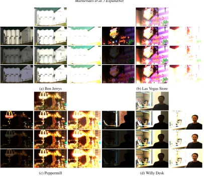
[image:10.595.55.289.463.641.2](a) Ben Jerrys (b) Las Vegas Store
[image:11.595.101.508.67.417.2](c) Peppermill (d) Willy Desk
Figure 14: Examples of expanded images using EXP and EIL at three different exposures. The examples are cropped from larger images, showing under various lighting conditions and from different scenes. The top row of each sub-figure shows the input LDR created with culling. The second row of each sub-figure shows the exposures of the original HDR. The following row shows exposures of predicted HDR using EIL. The last row shows exposures of predicted HDR using EXP.
We can further understand the architecture by comparing fig-ures3and13. The performance of Dilated + Global is comparable to that of Local + Global, even though figure3bis visually much better than3c. This is because the images from figure3are pre-dictions from an ExpandNet with all branches (some zeroed out when predicting), where the local and dilated branches have ac-quired separate scales of focus during training (high and medium frequencies respectively). In figure13, where each one is trained in-dividually, these scales are not separated; each branch tries to learn all the scales simultaneously. Separating scales in the architecture leads to improved performance.
6. Conclusions
This paper has introduced a method of expanding single expo-sure LDR content to HDR via the use of CNNs. The novel three branch architecture provides a dedicated solution for this type of problem as each of the branches account for different aspects of the expansion. Via a number of metrics it was shown that Ex-pandNet mostly outperforms the traditional expansion operators.
Furthermore, it performs better than non-dedicated CNN architec-tures based on UNT and COL. Compared to other dedicated CNN methods [EKD∗17,EKM17] it does well in certain cases, exhibit-ing fewer artefacts, particularly for content which is heavily under and over exposed. On the whole, ExpadNet is complementary to EIL which is designed to expand the saturated areas and does very well in such cases. Furthermore, EIL has a smaller memory foot-print. ExpandNet has shown that a dedicated architecture can be employed without the need of upsampling to convert HDR to LDR, however, further challenges remain. To completely remove arte-facts further investigation is required, for example in the receptive fields of the networks. Dynamic methods may require further care-ful design to maintain temporal coherence and Long Short Term Memory networks [HS97] might provide the solution for such con-tent.
Acknowledgements
References
[AFR∗07] AKYÜZA. O., FLEMINGR., RIECKEB. E., REINHARDE., BÜLTHOFFH. H.: Do HDR displays support LDR content?: A psy-chophysical evaluation. ACM Trans. Graph. 26, 3 (2007), 38. doi: http://doi.acm.org/10.1145/1276377.1276425.1,2,8
[AMS08] AYDINT., MANTIUKR., SEIDELH.-P.: Extending quality metrics to full luminance range images. InElectronic Imaging 2008 (2008), International Society for Optics and Photonics, pp. 68060B– 68060B.7
[BADC17] BANTERLE F., ARTUSI A., DEBATTISTAK., CHALMERS A.:Advanced High Dynamic Range Imaging. 2017.1,2,8
[BDA∗09] BANTERLEF., DEBATTISTAK., ARTUSIA., PATTANAIKS., MYSZKOWSKI K., LEDDAP., CHALMERSA.: High dynamic range imaging and low dynamic range expansion for generating HDR con-tent. InComputer graphics forum(2009), vol. 28, Wiley Online Library, pp. 2343–2367.2
[Ben09] BENGIOY.: Learning deep architectures for AI.Found. Trends Mach. Learn. 2, 1 (Jan. 2009), 1–127. URL:http://dx.doi.org/ 10.1561/2200000006,doi:10.1561/2200000006.1
[BLDC06] BANTERLEF., LEDDAP., DEBATTISTAK., CHALMERSA.: Inverse tone mapping. InGRAPHITE ’06: Proceedings of the 4th Inter-national Conference on Computer Graphics and Interactive Techniques in Australasia and Southeast Asia(New York, NY, USA, 2006), ACM, pp. 349–356.doi:http://doi.acm.org/10.1145/1174429. 1174489.2,8
[BVM∗17] BAKO S., VOGELS T., MCWILLIAMS B., MEYER M., NOVÁK J., HARVILLA., SENP., DEROSET., ROUSSELLEF.: Kernel-predicting convolutional networks for denoising monte carlo renderings. ACM Transactions on Graphics (TOG) 36, 4 (2017), 97.2
[CKS∗17] CHAITANYAC. R. A., KAPLANYANA. S., SCHIED C., SALVIM., LEFOHNA., NOWROUZEZAHRAID., AILAT.: Interactive reconstruction of monte carlo image sequences using a recurrent denois-ing autoencoder. ACM Transactions on Graphics (TOG) 36, 4 (2017), 98.2
[DBRS∗15] DEBATTISTAK., BASHFORD-ROGERST., SELMANOVI ´C E., MUKHERJEER., CHALMERSA.: Optimal exposure compression for high dynamic range content. The Visual Computer 31, 6-8 (2015), 1089–1099.8
[DD02] DURANDF., DORSEYJ.: Fast bilateral filtering for the display of high-dynamic-range images.ACM Trans. Graph. 21, 3 (July 2002), 257– 266. URL:http://doi.acm.org/10.1145/566654.566574,
doi:10.1145/566654.566574.6
[DLHT16] DONG C., LOY C. C., HE K., TANG X.: Im-age super-resolution using deep convolutional networks. IEEE Trans. Pattern Anal. Mach. Intell. 38, 2 (Feb. 2016), 295– 307. URL: http://dx.doi.org/10.1109/TPAMI.2015. 2439281,doi:10.1109/TPAMI.2015.2439281.2
[DMAC03] DRAGO F., MYSZKOWSKI K., ANNEN T., CHIBA N.: Adaptive Logarithmic Mapping For Displaying High Con-trast Scenes. Computer Graphics Forum 22, 3 (2003), 419– 426. URL: http://dx.doi.org/10.1111/1467-8659. 00689,doi:10.1111/1467-8659.00689.6
[DMHS08] DIDYK P., MANTIUKR., HEIN M., SEIDEL H.-P.: En-hancement of bright video features for HDR displays.Computer Graph-ics Forum 27, 4 (2008), 1265–1274.2
[EKD∗17] EILERTSEN G., KRONANDER J., DENES G., MANTIUK R. K., UNGERJ.: HDR image reconstruction from a single exposure using deep CNNs.ACM Trans. Graph. 36, 6 (2017), 1–10.2,8,11
[EKM17] ENDOY., KANAMORIY., MITANI J.: Deep Reverse Tone Mapping. ACM Transactions on Graphics (Proc. of SIGGRAPH ASIA 2017) 36, 6 (nov 2017).2,10,11
[Fai07] FAIRCHILDM. D.: The HDR photographic survey. InColor and Imaging Conference(2007), vol. 2007, Society for Imaging Science and Technology, pp. 233–238.6
[GN03] GROSSBERG M. D., NAYAR S. K.: What is the space of camera response functions? In2003 IEEE Computer Society Confer-ence on Computer Vision and Pattern Recognition, 2003. Proceedings. (June 2003), vol. 2, pp. II–602–9 vol.2.doi:10.1109/CVPR.2003. 1211522.10
[GPAM∗14] GOODFELLOWI., POUGET-ABADIE J., MIRZA M., XU B., WARDE-FARLEY D., OZAIR S., COURVILLE A., BENGIO Y.: Generative Adversarial Networks. InAdvances in Neural Informa-tion Processing Systems 27, Ghahramani Z., Welling M., Cortes C., Lawrence N. D., Weinberger K. Q., (Eds.). Curran Associates, Inc., 2014, pp. 2672–2680. URL:http://papers.nips.cc/paper/ 5423-generative-adversarial-nets.pdf.2
[HDQ17] HOUX., DUANJ., QIUG.: Deep feature consistent deep im-age transformations: Downscaling, decolorization and HDR tone map-ping. CoRR abs/1707.09482(2017). URL:http://arxiv.org/ abs/1707.09482.2
[HGSH∗17] HOLD-GEOFFROYY., SUNKAVALLIK., HADAPS.,
GAM-BARETTOE., LALONDEJ.-F.: Deep outdoor illumination estimation. In IEEE International Conference on Computer Vision and Pattern Recog-nition(2017).2
[HS97] HOCHREITER S., SCHMIDHUBER J.: Long Short-Term Memory. Neural Comput. 9, 8 (Nov. 1997), 1735–1780. URL:
http://dx.doi.org/10.1162/neco.1997.9.8.1735,
doi:10.1162/neco.1997.9.8.1735.11
[HYDB14] HUOY., YANGF., DONGL., BROSTV.: Physiological in-verse tone mapping based on retina response. The Visual Computer 30 (May 2014), 507–517.2,8
[HZRS15] HEK., ZHANGX., RENS., SUNJ.: Deep residual learning for image recognition. CoRR abs/1512.03385(2015). URL:http: //arxiv.org/abs/1512.03385.1
[IS15] IOFFES., SZEGEDYC.: Batch Normalization: Accelerating Deep Network Training by Reducing Internal Covariate Shift. InICML(2015), Bach F. R., Blei D. M., (Eds.), vol. 37 ofJMLR Workshop and Confer-ence Proceedings, JMLR.org, pp. 448–456.4
[ISSI16] IIZUKA S., SIMO-SERRA E., ISHIKAWA H.: Let there be Color!: Joint End-to-end Learning of Global and Local Image Priors for Automatic Image Colorization with Simultaneous Classification. ACM Transactions on Graphics (Proc. of SIGGRAPH 2016) 35, 4 (2016), 110:1–110:11.2,4,8
[ISSI17] IIZUKAS., SIMO-SERRAE., ISHIKAWAH.: Globally and lo-cally consistent image completion. ACM Trans. Graph. 36, 4 (July 2017), 107:1–107:14. URL: http://doi.acm.org/10.1145/ 3072959.3073659,doi:10.1145/3072959.3073659.2
[IZZE16a] ISOLAP., ZHUJ., ZHOUT., EFROSA. A.: Image-to-Image Translation with Conditional Adversarial Nets. Supplementary Ma-terial. https://phillipi.github.io/pix2pix/images/ cityscapes_cGAN_AtoB/latest_net_G_val/index. html, 2016.2
[IZZE16b] ISOLAP., ZHUJ., ZHOUT., EFROSA. A.: Image-to-image translation with conditional adversarial networks.CoRR abs/1611.07004 (2016). URL:http://arxiv.org/abs/1611.07004.2
[KB14] KINGMAD. P., BAJ.: Adam: A method for stochastic opti-mization.CoRR abs/1412.6980(2014). URL:http://arxiv.org/ abs/1412.6980,arXiv:1412.6980.7
[KBS15] KALANTARIN. K., BAKOS., SENP.: A machine learning ap-proach for filtering monte carlo noise.ACM Trans. Graph. 34, 4 (2015), 122–1.2
[KLL15] KIMJ., LEEJ. K., LEEK. M.: Deeply-recursive convolutional network for image super-resolution. CoRR abs/1511.04491(2015). URL:http://arxiv.org/abs/1511.04491.2
[KR17] KALANTARIN. K., RAMAMOORTHIR.: Deep high dynamic range imaging of dynamic scenes. ACM Trans. Graph. 36, 4 (July 2017), 144:1–144:12. URL: http://doi.acm.org/10.1145/ 3072959.3073609,doi:10.1145/3072959.3073609.2
[KSH17] KRIZHEVSKY A., SUTSKEVER I., HINTON G. E.: Ima-genet classification with deep convolutional neural networks. Commun. ACM 60, 6 (May 2017), 84–90. URL:http://doi.acm.org/10. 1145/3065386,doi:10.1145/3065386.5
[KUMH17] KLAMBAUERG., UNTERTHINERT., MAYRA., HOCHRE-ITERS.: Self-Normalizing Neural Networks. CoRR abs/1706.02515 (2017). URL:http://arxiv.org/abs/1706.02515.4
[Lan02] LANDISH.: Production-ready global illumination. In SIG-GRAPH Course Notes16 (2002), pp. 87–101.2,8
[MAF∗09] MASIAB., AGUSTINS., FLEMINGR. W., SORKINE O., GUTIERREZD.: Evaluation of reverse tone mapping through varying ex-posure conditions.ACM Trans. Graph. 28, 5 (2009), 1–8.doi:http: //doi.acm.org/10.1145/1618452.1618506.2,8
[MCL15] MATHIEU M., COUPRIE C., LECUN Y.: Deep multi-scale video prediction beyond mean square error. CoRR abs/1511.05440 (2015). URL:http://arxiv.org/abs/1511.05440.5
[MDK08] MANTIUKR., DALYS., KEROFSKYL.: Display adaptive tone mapping. ACM Trans. Graph. 27, 3 (2008), 1–10. doi:http: //doi.acm.org/10.1145/1360612.1360667.6
[MdPVA16] MARCHESSOUX C.,DE PAEPE L., VANOVERMEIRE O., ALBANIL.: Clinical evaluation of a medical high dynamic range dis-play. Medical Physics 43, 7 (2016), 4023–4031. URL:http://dx. doi.org/10.1118/1.4953187, doi:10.1118/1.4953187.
1
[MDS06] MEYLANL., DALYS., SÜSSTRUNKS.: The Reproduction of Specular Highlights on High Dynamic Range Displays. InIST/SID 14th Color Imaging Conference(Scottsdale, AZ, USA, 2006), pp. 333–338.
2
[MSG17] MASIAB., SERRANOA., GUTIERREZD.: Dynamic range expansion based on image statistics.Multimedia Tools and Applications 76, 1 (2017), 631–648.2
[NMDSLC15] NARWARIA M., MANTIUK R. K., DA SILVA M. P., LECALLETP.: HDR-VDP-2.2: a calibrated method for objective qual-ity prediction of high-dynamic range and standard images. Journal of Electronic Imaging 24, 1 (2015), 010501–010501.7
[ODO16] ODENA A., DUMOULIN V., OLAH C.: Decon-volution and checkerboard artifacts. Distill (2016). URL:
http://distill.pub/2016/deconv-checkerboard,
doi:10.23915/distill.00003.2,3
[pyt] PyTorch: Tensors and Dynamic neural networks in Python with strong GPU acceleration.http://pytorch.org/.7
[RD05] REINHARDE., DEVLINK.: Dynamic range reduction inspired by photoreceptor physiology. IEEE Transactions on Visualization and Computer Graphics 11, 1 (2005), 13–24.6
[RFB15] RONNEBERGER O., FISCHER P., BROX T.: U-Net: Con-volutional Networks for Biomedical Image Segmentation. CoRR abs/1505.04597(2015). URL:http://arxiv.org/abs/1505. 04597.2,8
[RHW86] RUMELHARTD. E., HINTONG. E., WILLIAMSR. J.: Learn-ing representations by back-propagatLearn-ing errors. Nature 323, 6088 (1986), 533–538.7
[RSSF02] REINHARDE., STARKM., SHIRLEYP., FERWERDAJ.: Pho-tographic tone reproduction for digital images. ACM Trans. Graph. 21, 3 (July 2002), 267–276. URL:http://doi.acm.org/10.1145/ 566654.566575,doi:10.1145/566654.566575.2
[RTS∗07] REMPELA. G., TRENTACOSTEM., SEETZENH., YOUNG
H. D., HEIDRICHW., WHITEHEADL., WARDG.: LDR2HDR: On-the-fly reverse tone mapping of legacy video and photographs. ACM Trans. Graph. 26, 3 (2007), 39. doi:http://doi.acm.org/10. 1145/1276377.1276426.2,8
[SBRCD17] SATILMIS P., BASHFORD-ROGERS T., CHALMERS A., DEBATTISTAK.: A machine-learning-driven sky model. IEEE Com-puter Graphics and Applications 37, 1 (Jan 2017), 80–91. doi:10. 1109/MCG.2016.67.2
[Sch14] SCHMIDHUBER J.: Deep learning in neural networks: An overview.CoRR abs/1404.7828(2014). URL:http://arxiv.org/ abs/1404.7828.1,3
[SCT∗16] SHI W., CABALLERO J., THEISL., HUSZARF., AITKEN
A. P., LEDIGC., WANGZ.: Is the deconvolution layer the same as a convolutional layer? CoRR abs/1609.07009(2016). URL:http: //arxiv.org/abs/1609.07009.3
[SHS∗04] SEETZEN H., HEIDRICH W., STUERZLINGER W., WARD G., WHITEHEAD L., TRENTACOSTE M., GHOSH A., VOROZ-COVS A.: High dynamic range display systems. In ACM SIG-GRAPH 2004 Papers(New York, NY, USA, 2004), SIGGRAPH ’04, ACM, pp. 760–768. URL: http://doi.acm.org/10.1145/ 1186562.1015797,doi:10.1145/1186562.1015797.1
[TR93] TUMBLINJ., RUSHMEIERH.: Tone reproduction for realistic images. IEEE Comput. Graph. Appl. 13, 6 (Nov. 1993), 42–48. URL:
http://dx.doi.org/10.1109/38.252554,doi:10.1109/ 38.252554.6
[WWZ∗07] WANGL., WEIL.-Y., ZHOUK., GUOB., SHUM H.-Y.: High dynamic range image hallucination. InSIGGRAPH ’07: ACM SIGGRAPH 2007 Sketches(New York, NY, USA, 2007), ACM, p. 72.
doi:http://doi.acm.org/10.1145/1278780.1278867.2
[YK15] YUF., KOLTUNV.: Multi-scale context aggregation by dilated convolutions. CoRR abs/1511.07122(2015). URL:http://arxiv. org/abs/1511.07122.4
[YKK17] YAMANAKAJ., KUWASHIMAS., KURITAT.: Fast and ac-curate image super resolution by deep CNN with skip connection and network in network. CoRR abs/1707.05425(2017). URL:http: //arxiv.org/abs/1707.05425.2
[ZL17a] ZHANGJ., LALONDEJ.-F.: Learning high dynamic range from outdoor panoramas. InIEEE International Conference on Computer Vi-sion(2017).2
[ZL17b] ZHANG J., LALONDE J.-F.: Learning High Dy-namic Range from Outdoor Panoramas. Supplementary Material.
![Table 1: Parameters used for tone mapping. All images are fol-lowed by a gamma correction curve with γ ∈ [1.8,2.2]](https://thumb-us.123doks.com/thumbv2/123dok_us/579919.557677/5.595.78.534.74.283/table-parameters-mapping-images-lowed-gamma-correction-curve.webp)