Adaptive neural network control of underactuated surface vessels with guaranteed transient performance: Theory and experimental results

(1)

Adaptive Neural Network Control of

Underactuated Surface Vessels with

Guaranteed Transient Performance: Theory and

Experimental Results

Lepeng Chen, Rongxin Cui,

Member, IEEE

, Chenguang Yang,

Senior Member, IEEE

, and Weisheng Yan

Abstract—In this paper, an adaptive trajectory track-ing control algorithm for underactuated unmanned surface vessels (USVs) with guaranteed transient performance is proposed. To meet the realistic dynamical model of USVs, we consider that the mass and damping matrices are not diagonal and the input saturation problem. Neural Networks (NNs) are employed to approximate the unknown external disturbances and uncertain hydrodynamics of USVs. More-over, both full state feedback control and output feedback control are presented, and the unmeasurable velocities of the output feedback controller are estimated via a high-gain observer. Unlike the conventional control methods, we employ the error transformation function to guarantee the transient tracking performance. Both simulation and experimental results are carried out to validate the superior performance via comparing with traditional potential inte-gral (PI) control approaches.

Index Terms—Neural Network, underactuated surface vessel, guaranteed transient performance.

I. INTRODUCTION

In the last decades, USV plays an important role in moni-toring, exploration, surveillance and military applications. The accurate trajectory tracking control of USVs is a challenge because the precise model is unavailable and the external dis-turbances, such as ocean waves, currents, upward or downward streams and tides, can deteriorate the control performance.

Several control approaches have been proposed to relieve the effect of unknown disturbances and model uncertainties, such as sliding mode control [1]–[3], adaptive backstepping control [4]–[9], NN-based control [10]–[13], and neural learn-ing control [14]–[16], model predictive control [17], [18], data-driven based control [19]–[21]. In [2], a novel sliding mode control strategy was presented for underactuated USV trajectory tracking by using a first-order and a second-order

Manuscript received October 17, 2018; revised February 01, 2019 and April 13, 2019; accepted April 18, 2019. This work was supported in part by the National Natural Science Foundation of China (NSFC) under grant U1813225, grant 61633002 and grant 61472325, and in part by the Science, Technology and Innovation Commission of Shenzhen Municipality under grant JCYJ20170817145216803, and in part by the Doctorate Foundation of Northwestern Polytechnical University under grant CX201904(Corresponding author: Rongxin Cui.)

L. Chen, R. Cui and W. Yan are with the School of Marine Science and Technology, Northwestern Polytechnical University, Xi’an 710072, China.(email: [email protected]).

C. Yang is with is with the Bristol Robotics Laboratory, University of the West of England, Bristol BS16 1QY, U.K.(e-mail: [email protected]).

sliding surface that based on surge and lateral tracking errors, respectively. In [6], an adaptive NN-based control for the realistic dynamical model of underactuated USVs that the mass and damping matrices are not diagonal was studied. In [22], to follow the sharp changing curvature, a path-following controller for USVs that based on disturbances observer was investigated. In [10], both full-state and output feedback adaptive neural control were proposed for USVs, and asymmetric barrier Lyapunov function was used to achieve output constraint. Based on the previous work, [14] presented an radial basis function (RBF) neural learning output feedback controller to steer an USV without velocity measurements. In [15], under the persistent excitation (PE) condition, a neural learning control of USVs was proposed with guaranteed per-formance. In [23], an online learning adaptive NN controller for small unmanned aerial rotorcraft was proposed to improve tracking performance via estimating the disturbances and elim-inating their adverse effects, and expermental results verified the proposed controller. In [24], a fuzzy adaptive controller with simple form was proposed, and the global stability was proved for the system that under the unmodelled dynamics. In [19], a model-free iterative controller was presented to enhance the tuning performance via the designed certerion and measured closed loop data. The above-mentioned control schemes achieve good performance to address the problem of model uncertainties, external disturbances, unavailable veloc-ity measurements, etc. Among these control techniques, the adaptive NN control is one of the most promising tools to improve the tracking performance of USVs that affected by the model uncertainties and disturbances.

(2)

In real applications, the USV may be influenced by many obstacles such as submerged rocks in ocean. To ensure the safety of USVs, we need to guarantee the tracking errors remaining in a prescribed bounded region. Moreover, uncon-strained maximum transient overshoot of the tracking errors can degrade the control performance, which may lead to a failing control. In addition, once the trajectory tracking errors violate the prescribed boundedness, in other words, the trans-formed errors become nonsense values, then USVs will stop working “automatically” , and it is a wonderful way to protect themselves. Therefore, guaranteeing transient performance is one of the most important issue and need to achieve in the control of USVs. In [26], a novel error transformation function was presented to restrict the maximum overshoot, convergence rate and steady-state error of strict feedback nonlinear systems with unknown nonlinearities. In [15], prescribed transient-performance-based neural learning controller was proposed to steer a fully actuated surface vessel with model uncertainties and disturbances. In [27], the tracking control problem with guaranteed transient performance was addressed for torpedo-like and unicycle-torpedo-like underactuated underwater vehicles. In [28], a multi-layer NN robust controller was proposed for underactuated underwater vehicle with external disturbances and unmodeled dynamics, and the transient performance was achieved. In [29], a novel path following controller was pro-posed for USV with prescribed performance, and the nonlinear disturbance observers were designed to estimate the unknown disturbances.

The above papers are based on the assumption that mass and damping matrices of USVs are diagonal. However, in real model of USVs, this assumption is not tenable because the their shapes are not always semi-submerged sphere. In [30], the authors firstly relaxed the above assumption via introducing a coordinate transformation, which is crucial for controlling the underactuated USV. In [31], using the above coordinate transformation, a distributed containment control for USVs were proposed via backstepping technique. Noted that the designed controller for USVs in [3] is verified by experiment, and other controllers in [2], [4], [6], [12], [14], [15], [22], [25], [29]–[31] are verified by simulations.

In this paper, experiments are carried out to verify the effec-tiveness of the proposed controller. The USV that investigated in this paper only owns an inertial measurement unit (IMU) and a global positioning system (GPS), which are equipped to measure the attitude angle and position, respectively. In such a case, there is no direct sensor to measure USV’ velocity. To overcome the problem, output feedback controllers for USVs were proposed in [6], [32], [33].

Based on the above discussions, the difficulties of USVs control are focused on the effects of unknown external dis-turbances, input saturation, underactuated dynamic constrict, coupled and uncertain dynamic. Also, in real applications, guaranteeing the transient and steady-state tracking behavior can be an effective method to ensure the USV’ safety. It is meaningful to solve the above-mentioned issues simultane-ously. Therefore, we design an adaptive NN control for an underactuated USV with guaranteed transient performance, and both the real dynamical model and the issue that without

velocity measurements are considered. Different from the control of fully actuated USVs with guaranteed transient performance in [5] and [10], we focus on the control law with underactuated manner. Also, compared with [4], we develop a NN-based controller that can guarantee the tracking errors’ transient and steady-state performance. Furthermore, unlike the results in [18] and [19], we develop the adaptive control without velocity measurements, which is much more matched the real applications. The difficulty of this work lies in the analysis of the control stability with rigorous mathematical theory when addressing both underactuated and transient per-formance guaranteed control problems. Moreover, performing lake experiments on the USV to verify the proposed controller is another difficulty.

The main contributions can be listed as follows.

1) A NN-based output feedback control is proposed for an underactuated USV that subject to the unknown ex-ternal disturbances with transient tracking performance guaranteed. The transient behavior can be achieved via stabilizing the logarithm-based transformed errors, and the unmeasurable velocities are estimated by an observer. 2) An adaptive compensating approach and a state transfor-mation are introduced to address the input saturation and dynamic coupled problems that existing in the realistic situation, respectively.

3) Rigorous theoretical analysis shows that all closed-loop signals are uniformly ultimately bounded (UUB) under the proposed control. Experimental studies are also car-ried out to validate the effectiveness of the proposed control.

The remainder of this paper is given as follows. Section II describes an underactuated USV dynamic and introduces some useful preliminaries. Section III proposes an adaptive NN controller for the underactuated USV with prescribed transient performance. Section IV and V show the simulational and experimental results, respectively.

II. PRELIMINARIES AND PROBLEM FORMULATION

A. Surface Vessel Dynamics

Motivated by [30], the nonlinear dynamics of the USV with unknown disturbances are provided as

˙

η=J(ψ)ν

Mν˙=−C(ν)ν−D(ν)ν+d+δ(τ) (1)

whereη= [x, y, ψ]>denotes the position and yaw angle in the earth-fixed frame, respectively, which are shown in Fig. 1;ν = [u, v, r]>represents velocity states in surgeu, swayv, and yaw rin the body-fixed frame;M =M> is a non-diagonal inertia matrix,CandDare total Coriolis and Centripetal acceleration matrix, and damping matrix, respectively; d = [du, dv, dr]>

denotes the unknown disturbance; The saturated control vector δ(τ) = [δ1(τ1),0, δ3(τ3)]> = [δ1(τu),0, δ3(τr)]>is defined as

δi(τi) =

 



τi,max, if τi> τi,max

τi, if τi,min≤τi≤τi,max

τi,min, if τi< τi,min

(3)

where i= 1,3,τ = [τ1,0, τ3]> = [τu,0, τr]>, τu andτr are

USV’ surge force and yaw moment, respectively; the bounds τi,max andτi,min are known. In addition, we define the dead-zero function as χ= [χu,0, χr]>=τ−δ(τ).

O _X

Y

b X b

Y

x

y b

O

[image:3.612.63.453.360.746.2]

\

Fig. 1. Navigation and body frames of an USV.

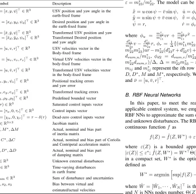
In practical applications, it is difficult to obtain the accurate hydrodynamics coefficients of USV. Thus, we divide the above matrices into nominal part and bias part, i.e.,M =M∗+∆M,

TABLE I

NOMENCLATURE

Symbol Description

η= [x, y, ψ]>_∈

R3 USV position and yaw angle in the

earth-fixed frame

ηd= [xd, yd, ψd]>∈R3 Desired position and yaw angle in the earth-fixed frame

¯

η= [¯x,y, ψ¯ ]>∈_R3 _{Transformed USV position and yaw} ¯

ηd= [¯xd,y¯d, ψa]>∈R3 Transformed Desired position and yaw angle

ν= [u, v, r]>∈_R3 _{USV velocities vector in the}

Body-fixed frame

νv= [uv, vv, rv]>∈R3 Virtual USV velocities vector in the body-fixed frame

¯

ν= [u,¯v, r]>∈_R3 _{Transformed USV velocities vector}

in the body-fixed frame

[xe, ye, ψe]>∈R3 Positional tracking errors

and yaw error

[ex, ey, eψ]>∈R3 Transformed tracking errors

[ρ1, ρ2, ρ3]>∈R3 Predefined bounded vector

δ(τ)∈_R3 _{Saturated control inputs vector}

τ= [τu,0, τr]>∈R3 Control inputs vector

χ= [χu,0, χr]>=τ−δ(τ) Dead-zero control inputs vector

J∈R3×3 Jacobian matrix

M, M∗,∆M Actual, nominal and bias part of inertia matrix

C, C∗,∆C Actual, nominal and bias part of Coriolis and Centripetal acceleration matrix

D, D∗_,_∆_D _{Actual, nominal and bias part} of damping matrix

d∈R3 Unknown external disturbances

w∈_R3 _{Time-varying disturbances}

in earth frame

dsum∈R3 Sum of disturbance and uncertainties

s1, s2, s3 Bias between virtual and

estimated/actual velocities

C = C∗ + ∆C and D = D∗+ ∆D, where the bias part

∆(·) denotes the difference between the real value and the nominal value, and(·)∗describes the nominal value that can be obtained from the tower tank experiment or the Computational Fluid Dynamics (CFD) analysis.

Remark 1:Unlike the conventional NN-based adaptive

con-trol for USV without any priori knowledge about the dynamics model parameters [19]–[21], we take full advantage of them to reduce the number of the NN node as well as computational complexity.

Now, the model of the USV can be rewritten as

M∗ν˙+C∗(ν)ν+D∗(ν)ν=δ(τ) +dsum (3) wheredsum =−∆Mν˙−∆C(ν)ν+d, and

J(ψ) =





cosψ −sinψ 0 sinψ cosψ 0

0 0 1



. (4)

Since the real USVs are not semi-submerged sphere, their dynamic model are coupled, namely, their mass and damping matrices can not be assumed as diagonal. In such cases, it is difficult to design the control and analyze the stability. Therefore, motivated by [30], the state transforming method is employed to transform the mass matrix to a diagonal form, i.e., v¯ = v+εr, x¯ = x+εcosψ, y¯ = y +εsinψ, and ε=m∗₂₃/m∗₂₂. The model can be rewritten as

˙¯

x=ucosψ−¯vsinψ, u˙ =φu+φd1+δ1(τu)/m

∗

11

˙¯

y=usinψ+ ¯vcosψ, v˙¯=φv+φd2

˙

ψ=r, r˙=φr+φd3+m

∗

22δ3(τr)/∆

(5) where φu =

m∗

22

m∗

11

vr+ m∗23

m∗

11

r2 ₋ d∗11

m∗

11

u, φv = −

m∗

11

m∗

22

ur −

d∗

22

m∗

22 v− d∗23

m∗

22

r, φr = _∆1{(m∗11m∗22−m∗22

2₎_uv_{+ (}_m∗

11m∗23− m∗22m∗23)ur−m∗22(d∗33r+d∗32v) +m∗23(d∗23r+d∗22v)},φd1= dsum,u/m∗11, φd2 = dsum,v/m∗22, φd3 = (−m∗23dsum,v +

m∗

22dsum,r)/∆, ∆ =m∗22m33∗ −m∗232; Furthermore, dij, d∗ij

mij andm∗ij represent theith row andjth column of matrices

D,D∗,M andM∗, respectively. We define thatη¯= [¯x,y, ψ¯ ]>

andν¯= [u,v, r¯ ]>.

B. RBF Neural Networks

In this paper, to meet the real-time requirement in the applicable control system, we employ a traditional one layer RBF NNs to approximate the sum of uncertain hydrodynamics and unknown disturbances. The RBF NNs can estimate the real continuous functionf as

f(Z) = ˆf(Z, W∗) +ε(Z), ∀Z∈Ω (6) where ε(Z) is a bounded approximation error satisfying |ε(Z)| ≤ε∗;fˆ(Z, W∗) =W∗>Θ(Z), the input vectorZ ∈Ω

in a compact set, W∗ is the optimal NNs weights and it is defined as

W∗= argminhsup|f(Z)−fˆ(Z,Wˆ)|i, Z∈Ω (7) whereWˆ = [ ˆW1,· · ·,WˆN]> is the weight parameter vector,

(4)

is the nonlinear regressor vector of the inputs, which has the form as

Θi(Z) = exp

−(Z−ξi)

>₍_Z₋_ξ_i)

σ2

i

, i= 1,· · · , N (8)

where ξi is the center of the ith basis function and σi

represents the variance of ith basis function.

C. Prescribed Transient Performance

We define the positional tracking errors and yaw error as xe, ye, ψe, respectively. To ensure the predefined transient

performance, i.e., overshoot and convergence rate, we have

−ρ1(t)< xe(t)< ρ1(t), ∀t≥0

−ρ2(t)< ye(t)< ρ2(t), ∀t≥0

−ρ3(t)< ψe(t)< ρ3(t), ∀t≥0

(9)

where ρi(t) is the predefined bounded function, which is described as

ρi(t) = (ρi,0−ρi,∞)e−α¯it+ρi,∞ i= 1, 2, 3 (10)

whereρi,0,ρi,∞ andα¯i are positive constants. The overshoot

and steady-state performance of tracking errorsxe,ye andψe

can be adjusted by the parameters of ρi,0 and ρi,∞. The α¯i

represents the predefined convergence rate.

To achieve the “constrained” tracking performance, the transformed errors are defined as

ex= Υ(x_ρ₁e), ey = Υ(_ρye₂), eψ= Υ(ψ_ρ₃e) (11)

Meanwhile, the performance bounding functionsΥin (11) can be chosen as

Υ(zi) = ln

1 +zi 1−zi

, i= 1,2,3 (12)

wherez1= x_ρe₁,z2=_ρye₂,z3=ψ_ρ₃e.

Remark 2: [31] The function Υ(zi) owns two characters:

Υ(zi) is a strictly increasing smooth function with bijective mappings Υ(·) : (−1,1)7→(−∞,∞), andΥ(0) = 0.

Lemma 1: [31] Consider the position and yaw errorsxe,ye,

ψe, and the transformed errors ex, ey, eψ. If the transformed

errors are bounded, the prescribed transient performance of ex, ey andeψ can be guaranteed.

D. Problem Formulation

The objective of this paper is to develop a suitable control inputτuandτrsuch that USV can track the desired trajectory

ηd and the tracking errors xe, ye and ψe can converge to a

predefined bounds.

Assumption 1: The reference trajectory is defined as η˙d =

J(ψd)νd, then we have x˙d = udcosψd −vdsinψd, y˙d =

udsinψd +vdcosψd, ψ˙d = rd. where ηd = [xd, yd, ψd]>,

νd = [ud, vd, rd]>. We assume that ud,vd,ψd and their first

derivatives are bounded. Furthermore, the external disturbance dis bounded.

Lemma 2: [34], [35] Since the saturation constraints of

control inputs, we have that the velocitiesu, v, rare belonging to a compact set and bounded. Then, it is reasonable to assume

that the functionφu, φv andφr are Lipschitz with respect to

the velocity ν.

Proof: According to hydrodynamic characteristic of

USVs, the matrixC(ν) +D(ν)is positive. Therefore,Mν˙ =

−(C(ν) +D(ν))ν+d+δ(τ) is a stable plant. Sinced and δ(τ)are bounded, we can draw a conclusion that the velocities

u, v, r are belonging to a compact set and bounded. Based on

the facts thatφu, φv andφrare continuous, we can infer that

these functions are Lipschitz with respect to the velocityν. Define the tracking error as

xe= ¯x−x¯d, ye= ¯y−y¯d, ψe=ψ−ψa (13)

wherex¯d=xd+εcosψd, y¯d =yd+εsinψd. Motivated by

[6], ψa is an angle that related to ψd, xe and ye, which is

defined as

ψa=βtanh(D2/a1) +ψd (1−tanh(D2/a1) (14)

wherea1 is a positive constant, andβ = tan−1−ye

−xe

,D=

p

x2

e+y2e.

III. MAIN RESULTS

Based on the above-mentioned preliminaries and useful lemmas, we will design a full-state feedback and an output feedback controller for underactuated USVs in this section, respectively. NNs are employed to approximate the unknown external disturbances and uncertain dynamics.

A. Adaptive Neural Network Control With Full-State Feedback

In this subsection, we will design a control law for USVs via using backstepping technique, which can guarantee the transient performance. Let us divide this control design phase into three steps: designing the appropriate virtual velocities, yielding the derivatives of transformed errors ex, ey and eψ,

deducing the derivatives of velocity errorss1, s2 ands3. Step 1: Design the appropriate virtual velocities to stabilize the transformed tracking errors. Motivated by [6], the errors between virtual and actual velocities can be defined as

s1=u−uv−α1tanhβ1, s2= ¯v−vv−α2tanhβ2,

s3=r−rv−α3tanhβ3

(15)

whereα1,α2andα3are positive constants,νv= [uv, vv, rv]>

are virtual controls.

To stabilize the transformed tracking error, νv can be

designed as

uv=−l1excosψ−l1eysinψ+ ˙¯xdcosψ+ ˙¯ydsinψ

vv=l1exsinψ−l1eycosψ−x˙¯dsinψ+ ˙¯ydcosψ

rv=−l2eψ+ ˙ψd

(16)

wherel1andl2are positive constants. Furthermore,β1, β2and β3 are given by

˙

β1= cosh2β1{−µuβ1−χu/m∗11}/α1

˙

β2= cosh2β2{Wˆ2>Θ2(Z)−l3s1+l3s2−l3s3+φv}/α2

˙

β3= cosh2β3{−µrβ3−m∗22χr/∆}/α3

(5)

with positive constants l3, µu andµr.

Remark 3: The virtual controlsuv, vv andrv are proposed

to stabilize the transformed tracking errors ex, ey and eψ

in kinematic level. Moreover, β1 and β3 are designed to compensate the effect of saturated inputs in (2), and β2 is proposed to deal with the problem of underactuation.

Step 2: Deduce the derivatives of transformed errors ex, ey

andeψ. Differentiating both side of (13) along (5), we have

˙

xe=ucosψ−v¯sinψ−x˙¯d

˙

ye=usinψ+ ¯vcosψ−y˙¯d ˙

ψe=r−ψ˙a

(18)

Using (12), we have u=s1+uv+α1tanhβ1,v¯=s2+

vv+α2tanhβ2, r =s3+rv+α3tanhβ3. Substitutingu,v¯ andr into (18), we have

˙

xe=(s1+uv+α1tanhβ1) cosψ

−(s2+vv+α2tanhβ2) sinψ−x˙¯d ˙

ye=(s1+uv+α1tanhβ1) sinψ

+ (s2+vv+α2tanhβ2) cosψ−y˙¯d ˙

ψe=(s3+rv+α3tanhβ3)−ψ˙a

(19)

Differentiating both side of (11), we have

˙

ex=

ρ1x˙e−xeρ1˙ (1−z2

1)ρ21 , e˙y=

ρ2y˙e−yeρ2˙ (1−z2

2)ρ22

, e˙ψ=

ρ3ψ˙e−ψeρ3˙ (1−z2

3)ρ23 (20)

Substituting (19) into (20), we have

˙

ex=

−2l1ex+ 2s1cosψ−2s2sinψ+ϕ1 %1

˙

ey =

−2l1ey+ 2s1sinψ+ 2s2cosψ+ϕ2 %2

˙

eψ =

−2l2eψ+ 2s3+ϕ3 %3

(21)

where%i = (1−zi2)ρi, i= 1,2,3,ϕ1= 2α1tanhβ1cosψ− 2α1tanhβ1sinψ + 2 ˙ρ1z1, ϕ2 = 2α2tanhβ2sinψ + 2α2tanhβ2cosψ−2 ˙ρ2z2,ϕ3= 2α3tanhβ3−2 ˙ψa+ 2 ˙ψd− 2 ˙ρ3z3.

Remark 4: From the definition of ϕi, i= 1,2,3, we have:

(i) |tanh(•)| ≤1,|sin(•)| ≤1, |cos(•)| ≤1; (ii) According to the Assumption 1, both terms of x˙¯d, y˙¯d and ψ˙a are

bounded; (iii) From (12) and (10), we have |Υ−1₍_·₎_{| ≤} ₁_,

|ρ˙i| ≤αi(ρi,0−ρi,∞),i= 1,2,3, respectively. We can draw

a conclusion that there exist positive constantsϕ¯1,ϕ¯2andϕ¯3 satisfying ϕ1≤ϕ¯1,ϕ2≤ϕ¯2 andϕ3≤ϕ¯3.

Step 3: Deduce the derivatives of velocity errors s1, s2,s3 and the controlsτu,τr. Differentiating both sides ofs1, s2, s3 in (15) along (17), we have

˙

s1= ˙u−u˙v+µuβ1+χu/m∗11

˙

s2= ˙¯v−v˙v−Wˆ2>Θ2(Z) +l3s1−l3s2+l3s3−φv ˙

s3= ˙r−r˙v+µrβ3+m∗22τr/∆

(22)

Because of the facts that τu = δ1(τu) +χu and τr =

δ3(τr) +χr, and substituting (5) into (22), we have

˙

s1=φu+φd1−u˙v+µuβ1+τu/m∗11

˙

s2=φd2−v˙v−Wˆ2>Θ2(Z) +l3s1−l3s2+l3s3

˙

s3=φr+φd3−r˙v+µrβ3+m∗22τr/∆

(23)

whereZ = [u, v, r, uv, vv, rv, ex, ey, eψ]> is the input of the

NNs.

Then, the control and adaptive laws are designed as

τu=m∗11

−l3s1−l3s2−Wˆ₁>Θ1(Z)−φu−µuβ1

τr= ∆

−l3s2−l3s3−Wˆ3>Θ3(Z)−φr−µrβ3

/m∗₂₂

˙ˆ

Wi = Γi

Θi(Z)si−κiWˆi

, i= 1, 2, 3

(24)

whereκi>0.

˙

s1=φd1−u˙v−l3s1−l3s2−Wˆ1>Θ1(Z)

˙

s2=φd2−v˙v−Wˆ2>Θ2(Z) +l3s1−l3s2+l3s3

˙

s3=φd3−r˙v−l3s2−l3s2−Wˆ3>Θ3(Z)

(25)

Define thatW₁∗>Θ1(Z)+1=φd1−u˙v,W2∗>Θ2(Z)+2= φd2−v˙v andW3∗>Θ3(Z) +3=φd3−r˙v, we have

˙

s1=−l3s1−l3s2−W˜₁>Θ1(Z) +1

˙

s2=l3s1−l3s2+l3s3−W˜2>Θ2(Z) +2

˙

s3=−l3s2−l3s3−W˜3>Θ3(Z) +3

(26)

whereW˜i= ˆWi−Wi∗,i= 1,2,3.

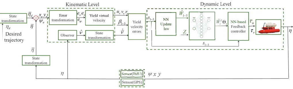
Remark 5:To further illustrate the proposed controller, we

draw a diagram in Fig. 2. The control scheme can be divided into kinematic and dynamic levels. In the kinematic level, we construct the virtual velocities to stabilize the transformational tracking errors. The goal of dynamic level is to ensure the virtual velocities can be tracked in the presence uncertainties via proposed control inputτu andτr.

Since the objectives of this controller are to ensure ex, ey, eψ, si,W˜i, i = 1,2,3 converge to the small

neighbor-hood of zero, then the Lyapunov function candidate can be defined as

V =V1+V2+V3 (27)

whereV1= 1₂%1e2

x+%2e2y+%3e2ψ,V2=

P3

i=1s 2

i andV3 =

P3

i=1W˜i>Γ

−1

i W˜i.

Theorem 1: Consider the USV dynamics in (1) and the

transformed dynamics in (5), together with the error trans-formed function in (11), the virtual controller in (16), the full-state feedback control and adaptive law in (24), and give the initial tracking error conditions that satisfying|ex(0)|< ρ1,0,

|ey(0)| < ρ2,0, |eψ(0)| < ρ3,0, the proposed full-state feedback controller can guarantee that: (i) the tracking errors are bounded by the prescribed functionρi and converge to a

small neighborhood of zero; (ii) the signals in the closed loop system are UUB.

Remark 6:In practice, there are two methods to ensure the

(6)

!!$ ! !$

! !$

"$

"!#$

!!$ ! !$

$ $

"!#$$

$ !$

$

!!$ ! !$

[image:6.612.51.560.58.213.2]

$

Fig. 2. Diagram of the proposed control system

algorithms can be utilized to yield an appropriate trajectory, which is in the neighborhood of the USV at the initial moment. By this method, we can guarantee the initial tracking errors in the predefined bounds. Also, appropriate choosing of the parameters ρ1,0,ρ2,0 andρ3,0 is another method to keep the initial tracking error in the bounds.

Proof: Taking the derivative of V1, and combing with

(21), we have

˙

V1=%1exe˙x+%2eye˙y+%3eψe˙ψ

=−2l1e2_x−2l1e2_y−2l2e2_ψ+ 2ex(s1cosψ−s2sinψ)

+ 2ey(s1sinψ+s2cosψ) + 2eψs3+exϕ1

+eyϕ2+eψϕ3+ ˙ρ1e2x/2 + ˙ρ2e2y/2 + ˙ρ3e2ψ/2

≤ −2l1e2x−2l1e2y−2l2e2ψ+ 2|exs1|+ 2|exs2|

+ 2|eys1|+|eys2|+ 2|eψs3|+|exϕ1¯ |+|eyϕ2¯ |

+|eψϕ3¯ |+ ¯%1e2x/2 + ¯%2e

2

y/2 + ¯%3e

2

ψ/2

(28)

Using the Young’s inequality, (28) can be rewritten as

˙

V1≤ −(2l1−5/2−

˙

%1

2 )e

2

x−(2l1−5/2−

˙

%2

2 )e

2

y

−(2l2−3/2−%3˙

2 )e

2

ψ+ 2

3

X

i=1 s2_i +1

2

3

X

i=1

¯

ϕ2_i (29)

Applying (26), V˙2 can be written as

˙

V2=s1(−l3s1−l3s2−W˜₁>Θ1(Z) +1)

+s2(l3s1−l3s2+l3s3−W˜2>Θ2(Z) +2)

+s3(−l3s2−l3s3−W˜3>Θ3(Z) +3)

=−l3 3

X

i=1 s2_i −

3

X

i=1

siW˜i>Θi(Z)−sii

(30)

There is an positive constant satisfying that i≤∗i. Since

sii ≤(s2i +i)/2, we have

˙

V2≤ −

l3−

1 2

3

X

i=1 s2_i −

3

X

i=1

siW˜i>Θi(Z)−

∗_i2

2

(31)

Using the adaptive law in (24), the derivatives ofV3can be written as

˙

V3=

3

X

i=1

ˆ

W_i>Θi(Z)si−κiWˆi

(32)

Applying the properties of RBFNN, we have

−κiW˜i>Wˆi≤

κi 2

kWi∗k

2

− kW˜ik2

(33)

˙

V3=

3

X

i=1

ˆ

W_i>Θi(Z)si+

κi 2kW

∗

ik

2₋κi 2k

˜

Wik2

(34)

Since %i ≤ρi,0, %˙i ≤%¯i, and combing (29), (31), (34), V˙

can be written as

˙

V ≤ −(2l1−5/2−%1/¯ 2)e_x2−(2l1−5/2−%2/¯ 2)e2_y

−(2l2−3/2−%¯3/2)e2ψ−(l3−5/2)s21−(l3−5/2)s22

−(l3−3/2)s23− 3

X

i=1 κi

2k ˜

Wik2+C

≤ −µV +C

(35)

where

µ= min

₂_l

1−5/2−%¯1/2 ρ1,0

,2l1−5/2−%¯2/2 ρ2,0

,

2l2−3/2−%3/¯ 2

ρ3,0

, l3−5/2,min

_κ

i

λmax(Γ−_i1)

C= 1

2

3

X

i=1

κikWi∗k

2₊∗2

i + ¯ϕ

2

i

where λmax(•) denotes the maximum eigenvalues of •. To guarantee the positive of µ, the control gains l1, l2 and l3 should be chosen to satisfy the following conditions:

l1≥max ( ¯%1/4 + 5/4,%2/¯ 4 + 5/4)

l2≥%¯3/4 + 3/4, l3≥5/2

(36)

Multiplying on both sides byeµt_{, we have}

(7)

From the above inequality, and applying the definition of V in (27), we can draw a conclusion that the transformed errorsex, ey, eψ,sias well as the NN weight estimation errors

˜

Wi are bounded. In terms of the boundedness of transformed

errors and according to Lemma 1, we can conclude that tracking error constraints xe, ye, ψe are never violated, i.e,

|xe(t)| < ρ1(t), |ye(t)| < ρ2(t), |ψe(t)| < ρ3(t). This completes the proof.

B. Adaptive Neural Network Control With Output Feed-back

The state-feedback control is based on the condition that the velocitiesu, v, rcan be measured via sensors, i,e., Inertial Navigation System (INS) or Doppler Velocity Log (DVL), etc. However, these sensors are too expensive. To deal with the problem, we employ a hign-gain observer to estimate the unmeasurable velocities. In this subsection, we will propose an output feedback control for the underactuated USV.

Consider the following system:

γb˙1=b2

γb2˙ =−λ1b2−b1+η (38)

whereγ is a small positive constant,b1, b2∈R3 are states.

Using the result of [8, Lemma 3] , ∃t > t∗, the estimate error b2

γ −η˙ is UUB. Therefore, we useb2/γ to estimateη˙.

According to the definition of J(ψ)in (4), we haveJ>=

J−1_{. Thus, the unmeasurable velocities}_ν_and_s_{= [}_{s1, s2, s3}_]>

can be estimated as

ˆ

ν=J>b2/γ, ˆs= ˆν−νv, ˜s= ˆs−s=J>ξ2 (39)

Using the full-state feedback control law in (24), we can rewrite the output feedback controller as

τu=m∗11

−l3ˆs1−l3sˆ2−Wˆ1>Θ1( ˆZ)−φˆu−µuβ1

τr= ∆

−l3ˆs2−l3ˆs3−Wˆ3>Θ3( ˆZ)−φˆr−µrβ3

/m∗22

˙ˆ

Wi= Γi

Θi( ˆZ)si−κiWˆi

, i= 1, 2, 3

(40)

whereZˆ = [ˆu,v,ˆ¯ ˆr, uv, vv, rv, ex, ey, eψ]>,κi>0 for alli= 1, 2, 3.

Theorem 2: Consider the USV dynamics in (1) and the

transformed dynamics in (5), together with the error trans-formed function in (11), the virtual controller in (16), the high-gain observer in (38), (39), the output feedback con-trol and adaptive law in (40), and give the initial tracking error conditions satisfy that |ex(0)| < ρ1,0, |ey(0)| < ρ2,0,

|eψ(0)|< ρ3,0, then the proposed full-state feedback controller can guarantee that: (i) the tracking errors are bounded by the prescribed function ρi and converge to a small neighborhood

of zero; (ii) the signals in the closed loop system are UUB.

Proof: The Lyapunov function V is defined in (27).

˙

s1=−l3sˆ1−l3sˆ2−φ˜u−Wˆ1>Θ1( ˆZ) +W1∗>Θ1(Z) +1

˙

s2=l3s1ˆ −l3s2ˆ +l3s3ˆ −φ˜v−Wˆ2>Θ2( ˆZ) +W2∗>Θ2(Z) +2

˙

s3=−l3s2ˆ −l3s3ˆ −φ˜r−Wˆ3>Θ3( ˆZ) +W3∗>Θ3(Z) +3 (41)

whereφ˜u= ˆφu−φu,φ˜v= ˆφv−φv andφ˜r= ˆφr−φr.

Applying (40), (26) and (21), theV˙ can be given as

˙

V =%1exe˙x+%2eye˙y+%3eψe˙ψ+

3

X

i=1 sis˙i+

3

X

i=1

˜

WiΓ−i1W˙˜i

=−2l1e2x−2l1e2y−2l2e2ψ−l3

3

X

i=1

s2i + 2ex(s1−s2)

+ 2ey(s1+s2) + 2eψs3+ 3

X

i=1

sigi(•) +exϕ1

+eyϕ2+eψϕ3+ ˙%1e2x+ ˙%2e

2

y+ ˙%3e

2

ψ

+

3

X

i=1

−siWˆi>Θi( ˆZ) +siWi∗>Θi(Z) +sii

+

3

X

i=1

˜

W_i>Θi( ˆZ)si−κiW˜i>Wˆi

(42)

whereg1(•) =−l3s1˜ −l3s2˜ −φ˜u,g2(•) =l3˜s1−l3˜s2+l3s3˜ − ˜

φv, g3(•) =−l3s2˜ −l3s3˜ −φ˜r. Using Lemma 2, under

As-sumption 1, we can conclude that there exist positive constants pi, i= 1,· · · ,4 satisfyingP

3

i=1sigi(•)≤P

3

i=1(pis2i) +p4. Applying the properties of RBF NN, we have

−κiW˜i>Wˆi≤

κi 2

kWi∗k2− kW˜ik2

kΘi( ˆZ)k ≤ξi, i≤∗i i= 1,2,3

(43)

whereξi,∗i are positive constants,%i≤ρi,0,%˙i≤%¯i.

Moreover, using the results of [10, Lemma 3] and [10, Lemma 4], we can conclude that there exist positive constants ςi, i= 1,2,3 satisfying

ˆ

Wi>Θi( ˆZ)−Wi∗>Θi(Z) =Wi∗>(Θi(Z)−Θi( ˆZ)) + ˜Wi>Θi( ˆZ)

≤W˜i>Θi( ˆZ) +kWi∗kζi

(44)

Using the Young’s inequality, (42) can be rewritten as

˙

V ≤ −(2l1−5/2−%¯1/2)ex2−(2l1−5/2−%¯2/2)e2y

−(2l2−3/2−%3/¯ 2)e2ψ−(l3−3−p1)s21

−(l3−3−p2)s22−(l3−2−p3)s23

−

3

X

i=1 κi

2k ˜

Wik2+C≤ −µV +C

(45)

where

µ= min

₂_l

1−5/2−%¯1/2 ρ1,0

,2l1−5/2−%¯2/2 ρ2,0

,

2l2−3/2−%¯3/2 ρ3,0

, l3−3−p1,

l3−3−p2, l3−2−p3,min

_κ

i

λmax(Γ−_i1)

C= 1

2

3

X

i=1

(κi+ςi2/2)kWi∗k

2₊∗2

i + ¯ϕ

2

i

(8)

where λmax(•) denotes the maximum eigenvalues of •. To guarantee the positive ofµ, the control gainl1, l2andl3should be chosen to satisfy the following conditions:

l1≥max ( ¯%1/4 + 5/4,%¯2/4 + 5/4), l2≥%¯3/4 + 3/4

l3≥max (3 +p1,3 +p2,2 +p3) (46)

Multiplying on both sides byeµt_{, we have}

V(t)≤(V(0)−C/µ) exp(−µt) +C/µ, ∀t >0 (47)

From the above inequality, and applying the definition of V in (27), we can draw a conclusion that the transformed errorsex, ey, eψ,sias well as the NN weight estimation errors

˜

Wi are bounded. In terms of the boundedness of transformed

errors and according to Lemma 1, we can conclude that tracking error constraints xe, ye, ψe are never violated, i.e,

|xe(t)| < ρ1(t), |ye(t)| < ρ2(t), |ψe(t)| < ρ3(t). This completes the proof.

Remark 7: The guidance on how to choose the control

parameters are shown as follows.

1) l1andl2 in the proposed control relate to the convergent rates of transformed positional errorsex, ey and angular

error eψ, respectively. Also, l3 is associated with the

convergent rates of velocity errors s1, s2 and s3. These parameters should be chosen as positive constants and satisfy the equations (36) and (47) to guarantee stability of the proposed algorithm.

2) ρi,0, ρi,∞ and α¯i are parameters in the predefined

bounded function. To avoid the sharp vibration in the beginning of tracking process, ρi,0 should be chosen enough large, and α¯i should be selected as small as

possible. Also, ρi,∞ can be suitable chosen according

to the accuracy of sensors and actuators that equipped in the USV.

3) α1 and α3 can influence the compensated rates of sat-urated inputs, and α2 will effect the rate to deal with underactuated problem. Moreover, γ is an important parameter for the high gain observer. If γ is selected very large, it will lead to a large estimation error at the beginning of control process.

IV. SIMULATIONS

To verify the effectiveness of the proposed controller, we use the USV model from Northwestern Polytechnical University, and these nominal parameters were identified by Unscented Kalman Filter (UKF) via experimental data. The high-gain observer, which is presented in (38) and (39), is designed to estimate the unmeasurable velocities. Logarithmic transformed errors are constructed in (11) to ensure the transient and steady tracking behavior. Furthermore, an adaptive compen-sating approach in (17) and an state transformation in (13) are designed to address the problems of input saturation, dynamic nonholonomic and dynamic coupled that existing in the realistic situation, respectively.

The nominal parameters are given as follows: (1) m∗11 =

141.85, m∗22 = 191.75, m∗23 = 5.7, m∗33 = 15.6, m∗12 =

m∗

21 = m∗13 = m∗31 = 0; (2) c∗13(v, r) = −191.75v −

5.7r, c∗₂₃(u) = 141.85u, c∗₃₁(vr) = 191.75v+ 5.7r, c∗₃₂(u) =

−141.85u, c∗₁₁ =c∗₁₂ =c∗₂₁ =c∗₂₂ =c∗₃₃ = 0; (3) d∗₁₁(u) = 45.6 + 67.26|u| + 10u2_{, d}∗

22(v, r) = 29.54 + 73.85|v| +

15|r|, d∗₂₃(v, r) =−2.5 + 2|v|+ 10.71|r|, d∗₃₂(v, r) =−2.4−

13|v| −0.2|r|, d∗₃₃(v, r) = 5.59 + 10.71|r| −0.07|r|, d∗₁₂ =

d∗₂₁=d∗₁₃=d∗₃₁= 0. Furthermore, the model uncertainty can be assumed as ∆(η, ν) = [0.5,0.1u2_,₀_.₁_r2_{+ sin(}_v_)]>_.

The desired trajectory is defined as follows: (1) 0 ≤ t <

100 : ud = 0.5, vd = 0, rd = 0; (2) 100 ≤ t < 300 :

ud = 0.5, vd = 0, rd = −0.005 sin(π(t −100)/400); (3) 300 ≤ t ≤ 700 : ud = 0.5, vd = 0, rd = −0.01/2. The

initial condition of the reference trajectory and the USV are ηd(0) = [0m,0m, π/4 rad]>, η(0) = [4m,−6m,0rad]>,

respectively. The predefined bounded functions are set as ρ1(t) = (20−2)e−0.05t+ 2, ρ2(t) = (20−2)e−0.05t+ 2, ρ3(t) = (3−π/9)e−0.05t+π/9.

To simulate the real oceanic environment, we define the time-varying disturbances in earth frame as

w(t) =





−8 + 1.8 sin(0.7t) + 1.2 sin(0.05t) + 1.2 sin(0.9t)

−4 + 0.4 sin(0.1t) + 0.2 cos(0.6t) 0





(48) Then, the disturbancesdacting on USV in body frame can be expressed asd(t) =J>(ψ)w(t).

We use RBFNN to approximate the unknown disturbance and uncertain dynamics. 512 NN nodes are used for each

Θi, and the initial weights Wi are zero. The gain

matri-ces are defined as Γi = 15I9×9 and the variances are chosen as σi = 8, where i = 1,2,3. The input

vec-tors of full back and output feedback controllers are de-signed as Z = [u,v, r, u¯ v, vv, rv, ex, ey, eψ]> and Zˆ = [ˆu,v,ˆ¯ ˆr, uv, vv, rv, ex, ey, eψ]>, respectively. The centres of the

neural networks nodes are evenly spaced between the upper and lower bound of the motion range and speed limits of each joint, namelyξi are evenly spaced on[0,0.75]×[−0.2,0.2]× [−0.04,0.04]×[0,0.75]×[−0.2,0.2]×[−0.04,0.04]×[−1,1]×

[−1,1]×[−1,1]. Moreover, to compare the control perfor-mance, a PI controller is designed as

τu=Kpu

p

x2

e+ye2+Kiu

Z p

x2

e+ye2dt

τr=Kprψe+Kir

Z

ψedt

(49)

whereKpu = 12,Kiu= 0.005,Kpr=−40,Kir= 0.

The gains of the adaptive NN control with full state feed-back are selected as l1 = 1, l2 = 2, l3 = 1, α1 = 30, α2 =

50, α3= 20,µu= 5, µr= 5, β1(0) = 0, β2(0) = 0, β3(0) =

0, κ1 = 3, κ2 = 1, κ3 = 6. Furthermore, the parameters of the adaptive NN control with output feedback are chosen as l1 = 1, l2 = 2, l3 = 1, α1 = 30, α2 = 50, α3 = 20, µu = 5, µr = 5, β1(0) = 0, β2(0) = 0, β3(0) = 0,

κ1= 3, κ2 = 6, κ3 = 12. Moreover, the parameters of high-gain observer are given as γ = 0.3, λ1 = 2, and the initial terms b1 = [0,0,0]>,b2= [0,0,0]>. The proposed full-state and output feedback control processes are defined as case 1 and case 2, respectively.

(9)

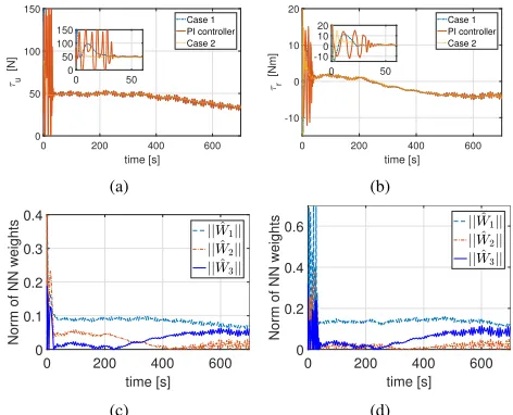
output feedback. From Figs. 3 (b-d), the tracking errors of the proposed controllers never violate the prescribed constraints, and the errors of the traditional PI controller can violate the prescribed bounds. Moreover, tracking errors of the proposed controllers will converge to a small value close to zero. Figs. 4 (a-b) give the control input τu and τr. The norms of NN

weights of two NN controllers, which are bounded with slight oscillations, are observed in Fig. 4 (c-d). Fig. 5 shows the observer errors, which indicate the proposed observer can estimate unmeasured velocities.

0 50 100 150 200 250

X(m) -50

0 50 100

Y(m)

Desired trajectory Case 1 PI controller Case 2

0 10 20

-10 0 10 20

(a)

0 200 400 600

time [s]

-20 -10 0 10 20

xe

[m]

Case 1 PI controller Case 2 Prescribed bounds

200 300 400 -0.5

0 0.5

(b)

0 200 400 600

time [s] -20

-10 0 10 20

ye

[m]

400 600 -20

2

(c)

0 200 400 600

time [s] -200

-100 0 100 200

e

[

°

]

500 600 700

-200

20 40

(d)

Fig. 3. (a)Trajectory in the horizontal plane. (b) Trajectory tracking error in X. (c) Trajectory tracking error in Y. (d) Trajectory tracking error inψ.

0 200 400 600

time [s]

0 50 100 150

u

[N]

Case 1 PI controller Case 2

0 50 0 50 100 150

(a)

0 200 400 600 time [s] -10

0 10 20

r

[Nm]

Case 1 PI controller Case 2

0 50 -100

10 20

(b)

0 200 400 600 time [s] 0

0.1 0.2 0.3 0.4

Norm of NN weights

(c)

0 200 400 600

time [s] 0

0.2 0.4 0.6

Norm of NN weights

(d)

Fig. 4. (a) Control input τu. (b) Control inputτr. (c) Norm of neural

weights for case 1. (d) Norm of neural weights for case 2.

V. EXPERIMENTS

In this section, we provide experimental results on an USV whose motion is controlled by two propellers. The experimen-tal system, as shown in Fig. 6, owns sensors including IMU and GPS, which are equipped to measure the attitude angle and position, respectively. To carry out the control, the USV runs a C++ program on a 1.8 GHz Industrial Personal Computer

0 100 200 300 400 500 600 700

-1 0 1

eu

[m/s]

0 100 200 300 400 500 600 700

0 1 2

ev

[m/s]

0 100 200 300 400 500 600 700

time [s] -0.5

0 0.5

er

[rad/s]

0 20 40

-1 0 1

0 20 40

0 1 2

0 50

[image:9.612.321.543.63.221.2]

-0.5 0 0.5

Fig. 5. Observer errors ofu, v,r.

(IPC) platform. The sensor, including IMU and GPS, updates its value every 0.01s, and the control implements every 0.1s. Furthermore, the supervisory computer system is designed to send the sailing mission and to surveillance the sailing states of the USV.

IMU +GPS

IPC

inet300

[image:9.612.60.293.184.367.2]

Supervisory Computer

Fig. 6. Illustration of the setup of the experiment.

The nominal parameters are identified by UKF via exper-imental data. The desired trajectory is initialized at ηd(0) = [5m,0m,0rad]>. The desired trajectory is defined as follows:

0 ≤ t ≤ 90 : ud = π/5, vd = 0, rd = π/100. The

bounded functions, hydrodynamic coefficients and input limits are defined the same as the ones in simulation part.

The gains of the experimental output feedback controller are selected as l1 = 1.8, l2 = 2.4, l3 = 1.9, α1 = 10, α2 =

30, α3= 20,µu= 5, µr= 5, β1(0) = 0, β2(0) = 0, β3(0) =

0, κ1 = 2.3, κ2 = 4.5, κ3 = 6. Moreover, the parameters of high-gain observer are given as γ = 0.1, λ1 = 1.2, and the initial terms b1 = [0,0,0]>, b2 = [0,0,0]>. The parameters of PI controller are chosen as Kpu = 16.2, Kiu = 0.002,

Kpr=−30,Kir= 0.

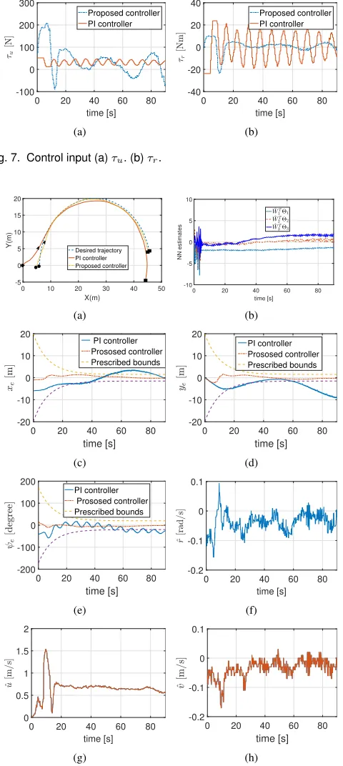
[image:9.612.322.550.333.501.2] [image:9.612.58.294.417.608.2]

(10)

controller with output state feedback. Fig. 8 (b) gives the estimated values of NNs. Fig. 7 gives the control input of two propellers. Figs. 8(c)-(e) describe that the tracking errors of the proposed controller never violate the prescribed constraints. Figs. 8(f)-(h) give the estimated values of state u, v, r.

0 20 40 60 80

time [s] -100

0 100 200 300

Proposed controller PI controller

(a)

0 20 40 60 80

time [s] -40

-20 0 20 40

Proposed controller PI controller

[image:10.612.57.297.129.665.2]

(b)

Fig. 7. Control input (a)τu. (b)τr.

0 10 20 30 40 50

X(m)

-5 0 5 10 15 20

Y(m)

Desired trajectory PI controller Proposed controller

(a)

0 20 40 60 80

time [s] -10

-5 0 5 10

NN estimates

(b)

0 20 40 60 80

time [s] -20

-10 0 10 20

PI controller Prososed controller Prescribed bounds

(c)

0 20 40 60 80

time [s] -20

-10 0 10 20

(d)

0 20 40 60 80

time [s] -200

-100 0 100 200

(e)

0 20 40 60 80

time [s] -0.2

-0.1 0 0.1

(f)

0 20 40 60 80

time [s] 0

0.5 1 1.5 2

(g)

0 20 40 60 80

time [s]

-0.2 -0.1 0 0.1

(h)

Fig. 8. Experimental results (a)Trajectory in X-Y plane, (b)estimated values of NN, (c)xe, (d)ye, (e)ψe, (f)rˆ, (g)uˆ, (h)vˆ.

VI. CONCLUSION

In this paper, an adaptive trajectory tracking controller with guaranteed transient performance is developed for a general

type of the USV. The NNs are used to approximate the unknown external disturbances and model uncertainties. To reflect more realistic situation, we simultaneously consider the input saturation problem and realistic dynamical model of the USV that the mass and damping matrices are not diagonal. Furthermore, simulation and experimental results show the superior performance of the proposed controller.

REFERENCES

[1] Z. Zhang, Y. Shi, Z. Zhang, and W. Yan, “New results on sliding-mode control for takagisugeno fuzzy multiagent systems,”IEEE Transactions on Cybernetics, vol. 49, no. 5, pp. 1592–1604, 2019.

[2] R. Yu, Q. Zhu, G. Xia, and Z. Liu, “Sliding mode tracking control of an underactuated surface vessel,”Control Theory & Applications, vol. 6, no. 3, pp. 461–466, 2012.

[3] H. Ashrafiuon, K. R. Muske, L. C. McNinch, and R. A. Soltan, “Sliding-mode tracking control of surface vessels,”IEEE Transactions on Industrial Electronics, vol. 55, no. 11, pp. 4004–4012, 2008. [4] M. Chen, S. S. Ge, B. V. E. How, and Y. S. Choo, “Robust adaptive

position mooring control for marine vessels,” IEEE Transactions on Control Systems Technology, vol. 21, no. 2, pp. 395–409, 2013. [5] L. Qiu, Y. Shi, J. Pan, B. Zhang, and G. Xu, “Collaborative tracking

control of dual linear switched reluctance machines over communication network with time delays,”IEEE Transactions on Cybernetics, vol. 47, no. 12, pp. 4432–4442, 2017.

[6] B. S. Park, J. W. Kwon, and H. Kim, “Neural network-based output feedback control for reference tracking of underactuated surface vessels,” Automatica, vol. 77, pp. 353–359, 2017.

[7] Z. Peng, J. Wang, and Q. L. Han, “Path-following control of autonomous underwater vehicles subject to velocity and input constraints via neu-rodynamic optimization,”IEEE Transactions on Industrial Electronics, 2019, doi:10.1109/TIE.2018.2885726.

[8] Z. Peng, J. Wang, and J. Wang, “Constrained control of autonomous underwater vehicles based on command optimization and disturbance estimation,”IEEE Transactions on Industrial Electronics, vol. 66, no. 5, p. 3627 3635, 2019.

[9] S. He, S. L. Dai, and F. Luo, “Asymptotic trajectory tracking control with guaranteed transient behavior for msv with uncertain dynamics and external disturbances,”IEEE Transactions on Industrial Electronics, vol. 66, no. 5, pp. 3712–3720, 2019.

[10] W. He, Z. Yin, and C. Sun, “Adaptive neural network control of a marine vessel with constraints using the asymmetric barrier lyapunov function,” IEEE transactions on cybernetics, vol. 47, no. 7, pp. 1641–1651, 2017. [11] X. Xiang, C. Yu, and Q. Zhang, “On intelligent risk analysis and critical decision of underwater robotic vehicle,”Ocean Engineering, vol. 140, pp. 453–465, 2017.

[12] Z. Peng, D. Wang, Z. Chen, X. Hu, and W. Lan, “Adaptive dynamic surface control for formations of autonomous surface vehicles with uncertain dynamics,”IEEE Transactions on Control Systems Technology, vol. 21, no. 2, pp. 513–520, 2013.

[13] L. Ding, S. Li, Y.-J. Liu, H. Gao, C. Chen, and Z. Deng, “Adaptive neural network-based tracking control for full-state constrained wheeled mobile robotic system,”IEEE Transactions on Systems, Man, and Cybernetics: Systems, vol. 47, no. 8, pp. 2410–2419, 2017.

[14] S. L. Dai, M. Wang, C. Wang, and L. Li, “Learning from adaptive neural network output feedback control of uncertain ocean surface ship dynamics,” International Journal of Adaptive Control & Signal Processing, vol. 28, no. 15, pp. 341–365, 2014.

[15] S. L. Dai, M. Wang, and C. Wang, “Neural learning control of marine surface vessels with guaranteed transient tracking performance,”IEEE Transactions on Industrial Electronics, vol. 63, no. 3, pp. 1717–1727, 2016.

[16] C. Yang, K. Huang, H. Cheng, Y. Li, and C. Y. Su, “Haptic identification by elm-controlled uncertain manipulator,”IEEE Transactions on Systems Man & Cybernetics Systems, vol. 47, no. 8, pp. 2398–2409, 2017. [17] C. Shen, Y. Shi, and B. Buckham, “Path-following control of an auv: A

multi-objective model predictive control approach,”IEEE Transactions on Control Systems Technology, vol. 27, no. 3, pp. 1334–1342, 2019. [18] ——, “Trajectory tracking control of an autonomous underwater vehicle

using lyapunov-based model predictive control,”IEEE Transactions on Industrial Electronics, vol. 65, no. 7, pp. 5796–5805, 2018.

(11)

[20] M.-B. Radac, R.-E. Precup, E. M. Petriu, and S. Preitl, “Iterative data-driven tuning of controllers for nonlinear systems with constraints,” IEEE Transactions on Industrial Electronics, vol. 61, no. 11, pp. 6360– 6368, 2014.

[21] Z. Wang, R. Lu, F. Gao, and D. Liu, “An indirect data driven method for trajectory tracking control of a class of nonlinear discrete-time systems,” IEEE Transactions on Industrial Electronics, vol. 64, no. 5, pp. 4121 – 4129, 2017.

[22] C. Hu, R. Wang, F. Yan, and N. Chen, “Robust composite nonlinear feedback path following control for underactuated surface vessels with desired-heading amendment,”IEEE Transactions on Industrial Electron-ics, vol. 63, no. 10, pp. 6386–6394, 2016.

[23] X. Lei, S. S. Ge, and J. Fang, “Adaptive neural network control of small unmanned aerial rotorcraft,”Journal of Intelligent & Robotic Systems, vol. 75, no. 2, pp. 331–341, 2014.

[24] S. Blai, I. Skrjanc, and D. Matko, “Globally stable direct fuzzy model reference adaptive control,”Fuzzy Sets & Systems, vol. 139, no. 1, pp. 3–33, 2003.

[25] J. Ghommam, F. Mnif, A. Benali, and N. Derbel, “Asymptotic backstep-ping stabilization of an underactuated surface vessel,”IEEE Transactions on Control Systems Technology, vol. 14, no. 6, pp. 1150–1157, 2006. [26] C. P. Bechlioulis and G. A. Rovithakis, “Brief paper: Adaptive control

with guaranteed transient and steady state tracking error bounds for strict feedback systems,”Automatica, vol. 45, no. 2, pp. 532–538, 2009. [27] C. P. Bechlioulis, G. C. Karras, S. Heshmati-Alamdari, and K. J.

Kyriakopoulos, “Trajectory tracking with prescribed performance for underactuated underwater vehicles under model uncertainties and exter-nal disturbances,”IEEE Transactions on Control Systems Technology, vol. 25, no. 2, pp. 429–440, 2016.

[28] O. Elhaki and K. Shojaei, “Neural network-based target tracking control of underactuated autonomous underwater vehicles with a prescribed performance,”Ocean Engineering, vol. 167, pp. 239–256, 2018. [29] Z. Zheng and M. Feroskhan, “Path following of a surface vessel with

prescribed performance in the presence of input saturation and external disturbances,”IEEE/ASME Transactions on Mechatronics, vol. 22, no. 6, pp. 2564–2575, 2017.

[30] K. D. Do and J. Pan, “Global tracking control of underactuated ships with nonzero off-diagonal terms in their system matrices,”Automatica, vol. 41, no. 1, pp. 87–95, 2005.

[31] S. J. Yoo and B. S. Park, “Guaranteed performance design for distributed bounded containment control of networked uncertain underactuated surface vessels,”Journal of the Franklin Institute, vol. 354, no. 3, pp. 1584–1602, 2017.

[32] L. P. Perera and C. G. Soares, “Pre-filtered sliding mode control for non-linear ship steering associated with disturbances,”Ocean Engineering, vol. 51, no. 3, pp. 49–62, 2012.

[33] L. J. Zhang, H. M. Jia, and X. Qi, “Nnffc-adaptive output feedback

Lepeng Chenreceived B.Eng. degree in auto-matic control from Northwestern Polytechnical University, Xi’an, China, in 2015.

He is currently pursuing the Ph.D. degree at the School of Marine Science and Tech-nology, Northwestern Polytechnical University, Xi’an, China. His research interests are adaptive control and its applications to marine vehicles.

trajectory tracking control for a surface ship at high speed,” Ocean Engineering, vol. 38, no. 13, pp. 1430–1438, 2011.

[34] S. Roy, S. B. Roy, and I. N. Kar, “Adaptive robust control of eulerla-grange systems with linearly parametrizable uncertainty bound,”IEEE Transactions on Control Systems Technology, vol. 26, no. 5, pp. 1842– 1850, 2018.

[35] C. Wen, J. Zhou, Z. Liu, and H. Su, “Robust adaptive control of uncertain nonlinear systems in the presence of input saturation and external disturbance,”IEEE Transactions on Automatic Control, vol. 56, no. 7, pp. 1672–1678, 2011.

Rongxin Cui (M’09) received the B.Eng. de-gree in autonomic control and the Ph.D. dede-gree in control science and engineering from North-western Polytechnical University, Xian, China, in 2003 and 2008, respectively.

From August 2008 to August 2010, he worked as a Research Fellow at the Centre for Offshore Research & Engineering, National University of Singapore, Singapore. Currently, he is a Pro-fessor with the School of Marine Science and Technology, Northwestern Polytechnical Univer-sity, Xi’an, China. His current research interests are control of nonlinear systems, cooperative path planning and control for multiple robots, con-trol and navigation for underwater vehicles, and system development.

Dr. Cui serves as an Editor for theJournal of Intelligent and Robotic Systemsand an Associate Editor for the IEEE TRANSACTIONS ON SYSTEMS, MAN, AND CYBERNETICS: SYSTEMS.

Chenguang Yang(M’10-SM’16) is a Professor of Robotics. He received the Ph.D. degree in control engineering from the National University of Singapore, Singapore, in 2010 and performed postdoctoral research in human robotics at Im-perial College London, London, UK from 2009 to 2010. He has been awarded EU Marie Curie International Incoming Fellowship, UK EPSRC UKRI Innovation Fellowship, and the Best Paper Award of the IEEE Transactions on Robotics as well as over ten conference Best Paper Awards. His research interest lies in human robot interaction and intelligent system design.