Fast and Discriminative Semantic Embedding
Rob Koopman OCLC Research [email protected]
Shenghui Wang OCLC Research
Gwenn Englebienne University of Twente
Abstract
The embedding of words and documents in compact, semantically meaningful vector spaces is a crucial part of modern information systems. Deep Learning models are powerful but their hyperpa-rameter selection is often complex and they are expensive to train, and while pre-trained models are available, embeddings trained on general corpora are not necessarily well-suited to domain specific tasks. We propose a novel embedding method which extends random projection by weighting and projecting raw term embeddings orthogonally to an average language vector, thus improving the dis-criminating power of resulting term embeddings, and build more meaningful document embeddings by assigning appropriate weights to individual terms. We describe how updating the term embed-dings online as we process the training data results in an extremely efficient method, in terms of both computational and memory requirements. Our experiments show highly competitive results with var-ious state-of-the-art embedding methods on different tasks, including the standard STS benchmark and a subject prediction task, at a fraction of the computational cost.
1
Introduction
Modern information systems rely extensively on the embedding of words and documents in compact, semantically meaningful vector spaces, where semantic similarity/relatedness can be computed and used efficiently. Various embedding methods are essentially all based on theDistributional Hypothesis (Har-ris, 1954; Sahlgren, 2008), and rely on co-occurrence evidence found in a corpus — whether computed globally or in a local context.
The recent success of local context predictive models such as Word2Vec (Mikolov et al., 2013) have initiated the development of more complex and powerful deep learning models (Bojanowski et al., 2016; Peters et al., 2018). The resulting embeddings combine compactness and discriminating ability, but the associated computational requirements are substantial and the optimal hyperparameter settings are not easy to find. It is, therefore, more common that embeddings are pre-trained on large corpora and plugged into a variety of downstream tasks (sentiment analysis, classification, translation, etc.). However, such transfer learning might fail to capture crucial domain-specific semantics.
In our approach, we use a two-step process where we first reduce the dimensionality of the term vectors by an extremely efficient implementation of random projection. We then project the term vectors on the hyperplane orthogonal to the average language vector, which improves how discriminative the vector representations are, and assign appropriate weights for building document embeddings.
The main contributions of this papers are:
• a method that computes the Random Projection of terms as expressed in terms of their co-occurrences in documents without storing the matrix of term co-occurrences,
• a method to compensate for uninformative language elements by projection on the hyperplane orthogonal to the average language vector,
• an effective weighing, adaptable to the domain and empirically verified, of the resulting vectors which optimises the discriminative power of terms, and
• on the whole, a practical method which requires no iterative parameter optimisation and computes embeddings and associated weights in a single pass through the documents of the training corpus.
As we show in our experiment section, the resulting method is highly competitive with the state-of-the-art, in terms of sentence similarity computation and downstream classification task, and has much lower computational space and time requirements.
2
Related work
Term embedding Much research has adopted the notion ofStatistical Semantics(Furnas et al., 1983; Weaver, 1955) or in Linguistics the Distributional Hypothesis(Harris, 1954; Sahlgren, 2008). Various distributional semantic models have been proposed to represent (embed) words in a continuous vec-tor space where semantically similar words are mapped to nearby points (‘are embedded nearby each other’). The approaches fall into two main categories (Baroni et al., 2014). First, methods based on global co-occurrence counts (e.g., Latent Semantic Analysis (Dumais, 2005)) which compute statis-tics of how often some word co-occurs with its neighbour words in a large text corpus, and then use dimensionality-reduction methods (e.g., Singular-Value Decomposition (Trefethen and Bau III, 1997), Random Projection (Achlioptas, 2003; Johnson and Lindenstrauss, 1984; QasemiZadeh et al., 2017)) to map the co-occurrence statistics of each word to a small, dense vector. Second, local context predic-tive methods (e.g. neural probabilistic language models) which directly try to predict a word from its neighbours or vice versa in terms of learned small, dense embedding vectors. The recent successes in the latter models, e.g. Word2Vec (Mikolov et al., 2013; Baroni et al., 2014) have initiated the development of more complex models with deep learning, such as FastText (Bojanowski et al., 2016), ElMO (Peters et al., 2018). However, that also brings high computational cost and complex parameters to optimise.
We propose a model that addresses these three issues: it is only trained on the training set; it does not require any optimisation (its computational time is linear in the size of the training set and can be implemented extremely efficiently); it uses linear projection to reduce the rank of the model. With only two straightforward parameters to tune — the term vectors’ dimensionality and the minimum threshold below which rare words are discarded — the simplicity of our model is also a desirable feature in practice.
3
Algorithm
Let a document be a set of words for which co-occurance is relevant,1 andnD be the total number of
documents and nV the number of frequent terms.2 A term is frequent when it occurs in more than
K documents in the corpus, whereK is flexible depending on the size of the corpus. As we show in Section 5.1.2, however, with the weightings we propose in our approach, K can be very low. Dis the chosen dimensionality of the embedding vectors.
Further, letva be theD-dimensional average vectorof the training documents. For each frequent
termt∈V, we have the following parameters:ct(d), The number of occurrences of termtin document
d;dt the number of documents that termtoccurs in; ~vt the raw embedding vector of termt;~rt a
D-dimensional “random vector” for termt,i.e.,~rtis a row ofR(In our approach, this vector is binary and
contains an equal number of +1 and -1);wtthe weight assigned to termtfor document embedding.
Algorithm 1Computing term embeddings
1: procedureCOMPUTING TERM EMBEDDINGS
2: ∀t:~vt←~0 .Initialise aD-dimensional zero vector for each termt
3: ∀t:wt←0 .Initial weight for each term is 0
4: ~va←~0 .Initialise aD-dimensional zero vector as the average vector
5: for alldocumentsddo
6: ~v←~0 .Initialise aD-dimensional zero vector
7: for alltermstin documentddo
8: δ← 1+log (√ct(d))
dt .Section 3.2
9: ~v←~v+δ ~rt .Section 3.1 and Section 3.2
10: for alltermstin documentddo
11: ~vt←~vt+~v .Section 3.1
12: ~va←~va+~v .Section 3.3
13: for alltermstdo
14: wt←1−cos(~vt, ~va) .Section 3.4
15: ~vt←~vt−(~vt·~va)~va .Section 3.3
16: ~vt∗←~vt/||~vt||2
3.1 Fast Random Projection
Traditional random projection starts by computing a matrix of (weighted) term co-occurrencesCof size nV ×nV, wherenV is the total number of terms. This matrix contains, for each pair of termsti and
tj, the number of documents (or paragraphs, or sentences) of the corpus in which bothti andtj occur.
Using a matrix of random projection vectorsRof sizenV ×D, we can then project ournV-dimensional
representation of each term to a lowerD-dimensional space:
C0[n
V×D]=C[nV×nV]R[nV×D] (1)
1
In this context, a document could therefore be a sentence, a paragraph, a fixed-size window, a bibliographic record,etc.
2Terms could be words or phrases. Common phrases are automatically detected using a method similar to that described by
However, computingC0requires us to store bothCandR, which can be challenging in terms of storage space and unacceptably expensive for large vocabularies. Instead, we propose a method to computeC0
without ever explicitly representingC, simply by leveraging the linear nature of the projection (Eq. 1), updatingC0 directly as we go through the corpus.
Algorithm 1 does this by decomposing C in Eq. 1 into the sum of individual documents’ co-occurrence matrices,C=P
dCd, so that
C0 =X
d
CdR (2)
where Cd is a matrix of zeros and ones indicating whether two terms co-occurred in the document.
Importantly, we can further decompose the matrix multiplication by relying on the properties of Cd:
every term in the document co-occurs equally with every other term in the document, so that all of the document’s terms contribute equally to the projection. We can, therefore, sum all the relevant rows ofR and add the result to the relevant rows ofC0, making the time complexity linear in the size of the corpus, and the space complexity linear in the vocabulary size and constant in the number of documents .
3.2 Weighted counts
To improve the robustness of the approach, we weight the co-occurrence matrix Cto reduce the effect of terms that are extremely common in certain documents and of terms that occur in the vast majority of documents. We use the term’s average modified TF.IDF score in the training documents. Experimentally, we verified that the traditional IDF term oflogdN
t suppresses frequent terms too much, and replace it by a factor ofpN/dt, which has a similar effect but a longer tail and can also be seen as the normalisation
constant of the t-test statistic (Manning and Sch¨utze, 1999). For the TF term, we use a factor of 1 + logct(d)and ignore the constantN which cancels out in the subsequent normalisation. Each row ofR
is therefore weighted accordingly in the decomposition outlined above.
3.3 Orthogonal projection
Traditional models discard both very infrequent words (because they are too rare for the model to be able to capture their semantics from the training data) and very frequent words (so-called “stop words” because they do not provide any semantically useful information). In our approach, we give a continuous weight to terms based on how frequently they occur and compute the average “language vector” of the corpus,~va. Unsurprisingly, this vector is very similar to the average vector of stop words. Intuitively,
words are increasingly more informative as they differ more from the average vector. By this reasoning, we project word vectors on the orthogonal hyperplane to~va(Algorithm 1 line 15),3resulting in a
repre-sentation where the uninformative component of terms is eliminated, and normalise the vectors to have unit length. When computing document vectors, we down-weight terms according to their similarity to ~
va(see Section 3.4). This step is crucial to get distinctive document embeddings.
As a nice side effect, projection makes it possible to handle multilingual corpora. The vocabulary of one language tends to be largely orthogonal to that of other languages (since words of one language tend to co-occur almost exclusively with words of the same language), so that projection using one language’s average vector does not have much effect on the terms in other languages. This makes it possible to handle different languages effectively, within the same vector space.
3.4 Term weight assignment
Using the projection described above, the component that differentiates a term from the average vector is kept as its final embedding. Similarly, how different a term is from~vaalso indicates how much that term
contributes to the semantics of a document it is part of. In fact, we can interpret the cosine similarity as
3
a lower bound on the mutual information (MI) between the two vectors (Foster and Grassberger, 2011). In order to give a higher weight to the most informative terms, we assign a higher weight to words with lower MI by setting the final weight of each term to bewt= 1−cos(~vt, ~va).
3.5 Text embedding
With the frequent terms’ embedding vectors and their proper weights, we can compute text embedding as the weighted average of its component term embeddings. For a text T, we obtain a set of vectors V ={~v∗t1, . . . , ~vt∗n}, wherenis the number of terms in textT and~vt∗i is the final embedding vector for termti. The embedding of textT is calculated as follows:
~ vd=
Pn
i=1wti·~v ∗
ti
Pn
i=1wti
. (3)
wherewti is the weight for termtiand out-of-vocabulary words are ignored. Note how term and docu-ment vectors all have unit length, making similarity computations elegant and effective.
4
Experimental methodology
We performed three experimental evaluations: in Experiment 1, we compare our method to the state-of-the-art on the standard STS benchmark; in Experiment 2, we qualitatively evaluate the weights assigned to terms; in Experiment 3, we evaluate our embedding method in terms of subject prediction. For our experiments, we implemented a parallelised version of the algorithm in C. All experiments were carried out on the same server with 2 Intel Xeon Silver 4109T 8-core processors and 384GB memory.
For meaningful evaluation, we trained all methods on the same two datasets using publicly available code for the state-of-the-art methods, and compared the resulting models on the standard STS benchmark. One dataset is the generic Simple English Wikipedia.4 The other domain-specific one is a subset of the MEDLINE database that consists of106MEDLINE articles, randomly selected fromWorldCat.org. In the latter dataset, each article is written in English and has a title and an abstract, to ensure sufficient textual information for computing the word embeddings. This dataset is of interest to our research and provides an interesting use case, as it consists of scientific articles and contains an above-average proportion of technical terms and jargon. Very rare terms carry critical meaning and make the task of word embedding particularly challenging.
5
Experimental results
5.1 Experiment I: STS Benchmark and Computational efficiency
The Semantic Textual Similarity (STS) Benchmark5 is a SemEval task organized between 2012 and 2017. It consists of 8628 pairs of English sentences, selected from image captions, news headlines and user forums. The similarity between these sentence pairs was annotated using a five point scale via crowdsourcing (Agirre et al., 2016). Participating systems calculate the similarity between these sentence pairs and are evaluated based on their Pearson correlation with the gold standard STS annotations.
We trained our method on the September 2018 datadump of Simple English Wikipedia, where we applied a sliding window of 80 terms, with 50% overlap. This resulted in 628,382 windows, each be-ing considered as a separate document for co-occurrence countbe-ing. A total of 199,430 unique 256-dimensional term vectors were obtained, their weights were calculated (Section 3.4), and used to embed the sentences in the STS benchmark (Section 3.5). The results are listed in Table 1, together with several state-of-the-art methods on the STS benchmark as published by Cer et al. (2017).
4
https://dumps.wikimedia.org/other/cirrussearch/20180910/
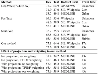
Table 1: STS scores and train times of different methods and different settings.
Method Dev Test Dataset used Train time
Doc2Vec (PV-DBOW) 72.2 64.9 AP-NEWS Unknown 31.0 27.0 S.E. Wikipedia 23m 53.7 49.8 MEDLINE 2h3m
FastText 65.3 53.6 Wikipedia Unknown
48.6 38.9 S.E. Wikipedia 51m 52.8 41.1 MEDLINE 3h4m
Sent2Vec 78.7 75.5 Twitter Unknown
68.8 62.2 S.E. Wikipedia 18m 65.4 55.0 MEDLINE 3h10m
Our method 75.1 64.6 S.E. Wikipedia 17s 73.6 58.9 MEDLINE 43s
Effect of projection and weighting in our method
No projection, no weighting 31.4 34.2 MEDLINE 43s No projection, TFIDF weighting 45.3 46.3 MEDLINE 43s With projection, no weighting 57.3 45.2 MEDLINE 43s With projection, TFIDF weighting 68.4 55.8 MEDLINE 43s With projection, our weighting 73.6 58.9 MEDLINE 43s
We then ran the publicly available implementations of Word2Vec (Mikolov et al., 2013), Doc2Vec (Le and Mikolov, 2014), GloVe (Pennington et al., 2014), FastText (Bojanowski et al., 2016) and Sent2Vec (Pagliardini et al., 2018) and trained them on the two datasets using the same machine. The common hyperparameters were chosen to generally maximise the different methods’ performance for this task, and are: a vector size of 256, a minimal number of word occurrences of 10, number of negative samples of 10, window size of 10, using hierarchical softmax, a learning rate of 1.0 and a number of threads of 16. All the other parameters were kept to their default values. When trained on the MEDLINE dataset, for word embedding only, it took Word2Vec and GloVe 29 and 35 minutes, respectively. As sentence-level embedding methods, Doc2Vec cost more than 2 hours to train. FastText and Sent2Vec also required more than 3 hours. In contrast, our combined term and document embedding — which includes the106
Medline articles and 340×103unique terms — requires only 43 s.
In analysing the STS benchmark results (Table 1), it is apparent that our method substantially outper-forms all baseline methods when trained on the same dataset. Also notice how the training dataset has a clear impact on each method’s performance, and even though the Simple English Wikipedia dataset is more limited, both in vocabulary and in size, than the datasets used for publication by the other meth-ods, our method still outperforms the published results of the other baselines in terms of STS scores, and is very competitive with Sent2Vec. All methods suffer a drop of performance on the generic STS benchmark when trained on the MEDLINE dataset, as a consequence of the domain-specific nature of the dataset, but this drop is least pronounced in the case of our method. This suggests that a careful search for a more appropriate training set would improve the method’s performance even further.
Finally, we should emphasise how low the train times are for our method. Since we do not require any iterative optimisation of the model parameters, our method’s results are deterministically determined by the training data, they do not depend on parameter initialisation, and training is orders of magnitudes faster than the other methods.
5.1.1 Effect of projection and weighting
We here report the effects of projection on the hyperplane orthogonal to~va(see Section 3.3) and
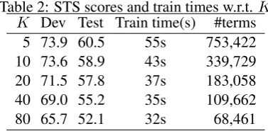
Table 2: STS scores and train times w.r.t.K K Dev Test Train time(s) #terms
5 73.9 60.5 55s 753,422 10 73.6 58.9 43s 339,729 20 71.5 57.8 37s 183,058 40 69.0 55.2 35s 109,662 80 65.7 52.1 32s 68,461
in terms of STS scores. Our weighting also substantially outperforms TFIDF weighting (both with and without projection), which itself outperforms no weighting. The difference in train time is negligible.
5.1.2 Effect ofK
Decreasing the thresholdKbelow which terms are ignored, results in a disproportionate increase of the number of terms that are included, with the computed vectors for those added terms being increasingly noisy. Because of the added computational burden and the noisiness of the estimation, traditionally a comparatively large cutoff value for K is chosen. With our proposed method, however, very small values forKare practical and the runtime does not grow much when a smallerK is chosen.
Table 2 reports the effect ofKon the STS benchmark and the corresponding runtime, when training with the 106 MEDLINE articles. With aK as small as 5, the runtime stays reasonable, while it brings real benefits in terms of the STS benchmark, beyond those reported in Table 1 (where all methods use K = 10), because more infrequent terms get embedded.
5.2 Experiment II: Qualitative evaluation of weights for individual terms
Table 3 gives examples of terms with their raw document counts and final weights. As expected, tradi-tionalstop words such as “for” and “also” have extremely low weights. Frequent terms such as “treat-ment,” “analysis,” “system,” and “subsequent” are to some extentdomain-specificstop words which have low semantic value and therefore low weights too. However, more meaningful ordiscriminativeterms such as “inflammatory,” “mRNA,” “antibodies” and “immune” have much higher weights even when they are also used very frequently.
At the other end of the spectrum, less frequent terms are likely to carry discriminative information for representing the semantics of the whole documents; however not all equally infrequent words have equally high weights. For example, “comprised” and “clarify” have much lower weights than “cytome-try,” “spleen,” “cox” and “embryos” which are expected to be key topics for documents which contain them. The orthogonal projection and weighting help to give discriminative terms a boost when calculat-ing the document embeddcalculat-ing, no matter how frequently these terms are used.
In addition, we observed that the average cosine similarity between all documents is smaller by orders of magnitude when orthogonal projection and weighting is performed compared to when it is not, suggesting the documents are distributed in more compact clusters. That being said, without a proper evaluation with domain experts, it is not easy to evaluate the genuine validity of such operation. Our future work will include conducting such user-in-the-loop evaluation.
5.3 Experiment III: Subject prediction
In most digital library catalogs, bibliographic records are indexed using controlled vocabularies or the-sauri to improve the discoverability of the content. These vocabularies are either generic, such as Library of Congress Subject Headings (LCSH),6or domain-specific, such as Medical Subject Headings (MeSH)7 which is used for indexing articles in the MEDLINE database. Traditionally, assigning a most relevant
6http://id.loc.gov/authorities/subjects.html
Table 3: Examples of term counts and their adjusted weights
t dt wt
for 720,776 0.003322 also 230,896 0.024318 treatment 171,984 0.079871 analysis 170,669 0.042365 system 99,582 0.077036 inflammatory 27,743 0.356823 mRNA 27,681 0.318550 achieved 27,382 0.114748 antibodies 27,379 0.433778 subsequent 27,289 0.060512
t dt wt
comprised 6099 0.293460 timing 6098 0.336269 artificial 6093 0.465012 cytometry 6086 0.776044 adjuvant 6085 0.501349 spleen 6080 0.523253 mucosal 6080 0.505713 cox 6072 0.608585 embryos 6055 0.724599 clarify 6053 0.298637
subset of subject headings to describe a record is done manually by professional taxonomists. However, such manual assignment is very time-consuming and can no longer keep up with the speed at which new records are produced. Therefore automatically assigning a set of relevant subjects to articles becomes increasingly important.
We evaluated our embedding method on the use case of subject prediction. This remains a difficult problem and is a form of Extreme Multi-label Text Classification (XMTC) (Prabhu and Varma, 2014; Bhatia et al., 2015; Liu et al., 2017), where the prediction space normally consists of hundreds of thou-sands to millions of labels and data sparsity and scalability are the major challenges. In our MEDLINE dataset, there are more than 324,619 MeSH headings indexing 896,300 articles (the other articles do not have any subjects) with on average 16 headings per article. However, only 102,484 MeSH headings are used to index more than 10 articles.
We propose to treat the MeSH headings as terms in the documents they are associated with, so that terms, documents and MeSH headings are all embedded in the same D-dimensional semantic space. Our assumption is that an article would be indexed by its most related subject headings,i.e., the MeSH headings with the highest cosine similarities to the document itself. To evaluate this, we computed embeddings for term and MeSH headings using the training dataset (previously selected 106MEDLINE articles). We then prepared a separate testing dataset which contains 104articles randomly selected from WorldCat.org. The articles in the testing dataset all have an abstract and are indexed by at least one MeSH heading. For each of these articles, we computed the document embedding using the terms in its title and abstract, following Eq. 3. We then computed their most similar MeSH headings and compared them with the actual ones. Notice how this method is, therefore, not biased towards predicting the more common (and often less informative) subjects.
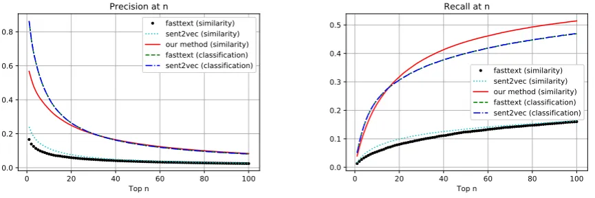
For FastText and Sent2Vec, we did the same,i.e., using the document-subject similarities to select the potential candidates. Since FastText and Sent2Vec can be used to train a supervised text classifier (Joulin et al., 2017), we additionally trained a classifier where each article’s title and abstract were concatenated as a text, and their actual MeSH subject headings were used as the labels to predict. We trained a separate FastText and Sent2Vec text classifier, which we used to predict the most likely subjects for the documents in the testing dataset, based on their title and abstract. The parameters for training a classifier were exactly the same as those for generating word embeddings, but the train time was dramatically shorter, less than 5 minutes with the same machine.
0 20 40 60 80 100 Top n
0.0 0.2 0.4 0.6 0.8
Precision at n
fasttext (similarity) sent2vec (similarity) our method (similarity) fasttext (classification) sent2vec (classification)
0 20 40 60 80 100
Top n 0.0
0.1 0.2 0.3 0.4 0.5
Recall at n
[image:9.595.92.525.79.223.2]fasttext (similarity) sent2vec (similarity) our method (similarity) fasttext (classification) sent2vec (classification)
Figure 1: The performance comparison when predicting subjects
quickly decreases to be almost the same as ours. Up to top 20 candidates, the recall for three methods are more or less the same, but our method is able to predict more actual subjects at lower ranks, where the recall outperforms FastText and Sent2Vec.
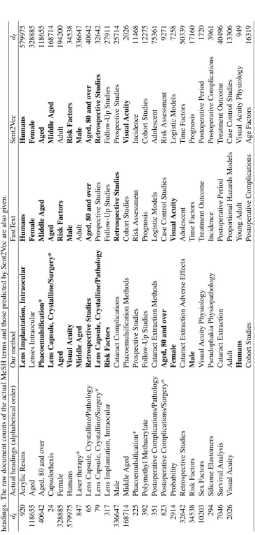
Table 4 lists the 23 actual MeSH headings of an example article.8 The MeSH terms that reflect the major points of this article are marked with an asterisk (*). The 25 most relevant MeSH headings pre-dicted by three methods are also listed. It is not surprising that subjects such as “Humans” and “Female” are predicted first by FastText and Sent2Vec, because they are the most frequent ones used in the training dataset. In fact, many of the subjects predicted by these two classifiers are very common (see their docu-ment counts in Table 4). These classifiers have trouble finding subjects which describe the articles more precisely, while our method ranks specific subjects such as “Lens Capsule, Crystalline/Surgery” high in the list, even though fewer than 100 articles in the training set are indexed by this subject.
We realise that this evaluation has its limitations. As shown in Table 4, highly related MeSH headings such as “Lenses Intraocular” and “Phacoemulsification Methods” are predicted as good candidates for this article, both of which are reasonable and potentially useful. But since they are not the subject headings that the professional taxonomists have chosen, their value cannot be easily assessed. This illustrates how precision/recall may not be a very meaningful evaluation metric in this application. It also shows how this method could provide good recommendations to cataloguers.
6
Conclusion
We have described a novel, simple, effective and efficient method for term and document embeddings. As we have shown, our method has important practical benefits: 1) it is fast and has low hardware requirements, having linear time complexity and constant space complexity in function of the number of documents, resulting in very short run-times in practice. 2) Since no iterative optimisation is needed, the resulting embeddings are not affected by parameter initialisation and there is no uncertainty about the quality of the results of a run. 3) It computes semantically discriminative term embeddings and weightings with a single pass through the training data, and has the capacity to effectively include very rare words. Our experiments show it outperforms state-of-the-art methods in terms of the STS benchmark and subject prediction when trained on the same datasets, while at the same time being computationally cheaper by orders of magnitude.
In the future, we will integrate sub-word information into the embedding process and evaluate how effectively previously unseen words can be embedded. We will consider a wider variety of evaluation methods, especially getting domain experts involved.
References
Achlioptas, D. (2003). Database-friendly random projections: Johnson-Lindenstrauss with binary coins.
Journal of Computer and System Sciences 66(4), 671–687.
Agirre, E., C. Banea, D. Cer, M. Diab, A. Gonzalez-Agirre, R. Mihalcea, G. Rigau, and J. Wieb (2016). Semeval-2016 task 1: Semantic textual similarity, monolingual and cross-lingual evaluation. In Pro-ceedings of the SemEval-2016.
Arora, S., Y. Liang, and T. Ma (2017). A simple but tough-to-beat baseline for sentence embeddings. In
Proceedings of 6th International Conference on Learning Representations. Poster.
Baroni, M., G. Dinu, and G. Kruszewski (2014). Don’t count , predict ! A systematic comparison of context-counting vs . context-predicting semantic vectors. Proceedings of the 52nd Annual Meeting of the Association for Computational Linguistics., 238–247.
Bhatia, K., H. Jain, P. Kar, M. Varma, and P. Jain (2015). Sparse local embeddings for extreme multi-label classification. In C. Cortes, N. D. Lawrence, D. D. Lee, M. Sugiyama, and R. Garnett (Eds.),
Advances in Neural Information Processing Systems 28, pp. 730–738. Curran Associates, Inc.
Bojanowski, P., E. Grave, A. Joulin, and T. Mikolov (2016). Enriching word vectors with subword information. arXiv preprint arXiv:1607.04606.
Cer, D., M. Diab, E. Agirre, I. Lopez-Gazpio, and L. Specia (2017). Semeval-2017 task 1: Semantic textual similarity multilingual and crosslingual focused evaluation. InProceedings of the 11th Inter-national Workshop on Semantic Evaluation (SemEval-2017), Vancouver, Canada, pp. 1–14.
Conneau, A., D. Kiela, H. Schwenk, L. Barrault, and A. Bordes (2017). Supervised learning of universal sentence representations from natural language inference data. InProceedings of the 2017 Conference on Empirical Methods in Natural Language Processing, pp. 670–680. Association for Computational Linguistics.
Dumais, S. T. (2005). Latent semantic analysis. Annual Review of Information Science and Technol-ogy 38, 188–230.
Foster, D. V. and P. Grassberger (2011, Jan). Lower bounds on mutual information. Phys. Rev. E 83, 010101.
Furnas, G. W., T. K. Landauer, L. M. Gomez, and S. T. Dumais (1983). Statistical semantics: Analysis of the potential performance of keyword information systems. Bell System Technical Journal 62(6), 17531806.
Harris, Z. (1954). Distributional structure. Word 10(23), 146162.
Johnson, W. and J. Lindenstrauss (1984). Extensions of Lipschitz mappings into a Hilbert space. Con-temporary Math. 26, 189–206.
Joulin, A., E. Grave, P. Bojanowski, and T. Mikolov (2017). Bag of tricks for efficient text classification. InProceedings of the 15th Conference of the European Chapter of the Association for Computational Linguistics: Volume 2, Short Papers, pp. 427–431. Association for Computational Linguistics.
Le, Q. V. and T. Mikolov (2014, 5). Distributed Representations of Sentences and Documents. Interna-tional Conference on Machine Learning - ICML 2014 32, 11881196.
Manning, C. D. and H. Sch¨utze (1999). Foundations of Statistical Natural Language Processing. Cam-bridge, MA, USA: MIT Press.
Mikolov, T., I. Sutskever, K. Chen, G. Corrado, and J. Dean (2013). Distributed representations of words and phrases and their compositionality. InProceedings of the 26th International Conference on Neural Information Processing Systems - Volume 2, NIPS’13, USA, pp. 3111–3119. Curran Associates Inc.
Moody, C. E. (2016, May). Mixing Dirichlet Topic Models and Word Embeddings to Make lda2vec.
arXiv e-prints, arXiv:1605.02019.
Pagliardini, M., P. Gupta, and M. Jaggi (2018). Unsupervised learning of sentence embeddings using compositional n-gram features. InProceedings of the 2018 Conference of the North American Chapter of the Association for Computational Linguistics: Human Language Technologies, Volume 1 (Long Papers), pp. 528–540. Association for Computational Linguistics.
Pearson, K. (1901). Liii. on lines and planes of closest fit to systems of points in space. The London, Edinburgh, and Dublin Philosophical Magazine and Journal of Science 2(11), 559–572.
Pennington, J., R. Socher, and C. D. Manning (2014). GloVe: Global vectors for word representation. In
Empirical Methods in Natural Language Processing (EMNLP), pp. 1532–1543.
Peters, M. E., M. Neumann, M. Iyyer, M. Gardner, C. Clark, K. Lee, and L. Zettlemoyer (2018). Deep contextualized word representations. In Proceedings of the 16th Annual Conference of the North American Chapter of the Association for Computational Linguistics: Human Language Technologies.
Prabhu, Y. and M. Varma (2014). Fastxml: A fast, accurate and stable tree-classifier for extreme multi-label learning. InProceedings of the 20th ACM SIGKDD International Conference on Knowledge Discovery and Data Mining, KDD ’14, New York, NY, USA, pp. 263–272. ACM.
QasemiZadeh, B., L. Kallmeyer, and A. Herbelot (2017). Non-negative randomized word embeddings. InProceedings of Traitement automatique des langues naturelles (TALN2017).
Roweis, S. T. and L. K. Saul (2000). Nonlinear dimensionality reduction by locally linear embedding.
science 290(5500), 2323–2326.
Sahlgren, M. (2008). The distributional hypothesis. Rivista di Linguistica 20(1), 3353.
Trefethen, L. N. and D. Bau III (1997). Numerical linear algebra. Philadelphia: Society for Industrial and Applied Mathematics.