A method for quantifying the absolute accuracy and precision of dynamic contrast enhanced MRI acquisition techniques

A method for quantifying the absolute

accuracy and precision of dynamic contrast

enhanced MRI acquisition techniques

Submitted in accordance with the requirements for the degree of

Doctor in Philosophy

in School of Medicine, Clinical Medicine

April 2018

by

Declaration

I declare that this thesis has not been submitted as an exercise for a degree at this or any other university and it is entirely my own work.

I agree to deposit this thesis in the University’s open access institutional repository or allow the library to do so on my behalf, subject to Irish Copyright Legislation and Trinity College Library conditions of use and acknowledgement.

________________________ Silvin Paul Knight

Summary

To data a method has been lacking which allows for the quantitative evaluation of the accuracy and precision of dynamic contrast-enhanced (DCE) MRI techniques, as implemented at the MR scanner, with results calculated against precisely-known ‘ground truth’ values. In this thesis a novel anthropomorphic dynamic phantom test device is presented which mimicked the male pelvic-region (in terms of size and complexity) within which ground truth contrast agent concentration time-intensity curves (CTCs) were generated and presented to the MRI scanner for measurement, thereby allowing for an assessment of a particular DCE-MRI protocol’s ability to repeatedly and accurately measure a given physiologically-relevant curve-shape. The device comprised of a 4-pump flow system, wherein CTCs derived from prior patient prostate data were produced for measurement at chambers placed within the imaged volume. The ground truth was determined using a highly-precise, MRI-independent, custom-built optical imaging system. Initial experiments performed using this system measuring prostate-tissue-mimicking CTCs (with a model population-averaged arterial input function (AIF)) at various temporal resolutions (Tres: the temporal spacing

between successive DCE measurements) and revealed significant errors in MRI-measured pharmacokinetic (PK) modelling outputs, amounting to values of up to 42%, 31%, and 50% for Ktrans (volume transfer coefficient), ve (extravascular-extracellular space volume fraction), and kep (rate constant) respectively. Further DCE-MRI experiments were performed wherein the Tres was varied in the range [2 - 24.4 s] and the acquisition duration (AD: the length of time that the CTCs were sampled for) in the range [30 - 600 s]. The phenomenological parameter ‘wash-in’ derived from the CTCs gave underestimation errors up to 40% when using Tres values  16.3 s; however, the measured ‘wash-out’ rate did not vary greatly across all Tres values tested. Errors in all derived PK parameter values were <14% for acquisitions with Tres 8.1s, AD 360s, but increased dramatically outside of this range.

The phantom test device was further used to investigate the effects of Tres, as well as B1+-field non-uniformities, on the accuracy and precision of simultaneously-measured AIF and prostate-tissue-mimicking CTCs, and derived PK parameters. A population-average AIF was established from the mean of 32 prostate patient dataset

measurements (Tres = 3.1 s), and this formed the basis for the ground truth AIF used. The phantom device was modified to allow for a ‘thin slab’ 3D-volume to be acquired with a Tres approaching 1 s using a standard spoiled gradient echo sequence. Five repeat intra-session and five inter-session AIF measurements were made

range [1.2 – 30.6 s], providing a total of 450 full DCE-MRI datasets for analysis. Flip angle errors deriving from B1+-field non-uniformities of -29% to -33% were measured. Performing voxel-wise flip-angle correction (VFAC) on the data to correct for this effect increased the PK parameter estimation accuracy by 12.9%, 9.2% and 20.2% for Ktrans, ve and kep respectively, and increased intra-session precision by up to 11.2%. It was also demonstrated that the use of a linear implementation of the standard Tofts PK model, rather than the more traditionally-used non-linear form, almost doubled the accuracy of Ktrans estimates, caused an increase in Ktrans and kep precision of 4%, and relaxed the dependence of the parameter accuracy on the Tres used.

A final set of experiments using the phantom system investigated the effect of under-sampling the data on the accuracy and precision of the measured CTCs and AIF, and the derived PK parameters. The data was acquired using a continuous golden-angle (GA) radial k-space trajectory and subsequently reconstructed using three approaches: (i) no parallel imaging (PI) or compressed sensing (CS) (i.e. coil-by-coil (CbC) inverse gridding), (ii) PI only, and (iii) PI combined with CS (PICS). Overall, the PICS

reconstruction approach was shown to provide the highest accuracy for PK parameter estimation, with all errors in Ktrans, ve, and kep parameter values less than 12%, 6.6%, and 12%, respectively, for data reconstructed with as little as 3% of the data required to fulfil the Nyquist criterion. This corresponds to a twenty-one-fold gain in acquisition speed, compared to a standard fully-sampled Cartesian approach with the same acquisition spatial resolution and geometries. PICS reconstruction was shown to provide a gain in accuracy in PK parameter estimations of up to 34% and 42% compared with the PI and CbC approaches, respectively.

Across the breadth of this thesis various factor which influence the absolute accuracy and precision on PK parameter estimations have been systematically and quantitatively investigated, refining the methodologies used, and ultimately arriving at an acquisition and data processing protocol which provided PK parameter estimations with mean errors all  2%, and with intra- and inter-session precision of  4% . This protocol comprises of a continuous GA radial acquisition with 100% radial sampling density, VFAC applied, and with linear fitting of the standard Tofts model to the measured data. However, the phantom device presented in this thesis allows for the quantitative

Acknowledgments

I would like to acknowledge and express my sincere gratitude to the following people:

My PhD supervisor, Prof Andrew Fagan, National Centre for Advanced Medical Imaging (CAMI), St James Hospital / Trinity College, University of Dublin (Dublin, Ireland), who provided me with the guidance, tools, and freedom to pursue my

research directions that were necessary in order to complete this research. Thank you Andrew for your unfaltering day-to-day support and dedication to the project; I could not have hoped for a better mentor.

The Irish Cancer Society (Dublin, Ireland), this work was funded by an Irish Cancer Society Research Scholarship, supported by The Movember Foundation [grant number CRS13KNI].

Prof Jacinta Browne, Dublin Institute of Technology (Dublin, Ireland), for her assistance with the production of the tissue-mimicking-materials used in the construction of the phantom, as well as her invaluable advice and expertise when designing the phantom system.

Prof David Smith, Vanderbilt University (Nashville, TN, USA), for his partial-supervision of my work during a 3-month period spent conducting part of this research at Vanderbilt University, as well as his mentorship with regards implementing various DCE-MRI reconstruction methods and pharmacokinetic analysis technique. I would also like to thank Prof Thomas Yankeelov for hosting me at Vanderbilt, and Prof Brian Welch for his advice and assistance.

Dr Matthew Clemence, Philips Healthcare (UK), for his assistance with implementing the continuous golden-angle radial acquisition protocol on the scanner.

Dr Sean Cournane, St James’s Hospital (Dublin, Ireland), for his assistance with initial attempts to measure the ground truths for the phantom system using X-ray.

My colleagues in the Imaging Physics Group, Trinity College, University of Dublin (Dublin, Ireland), for their feedback on the project at our monthly group-meetings, as well as moral and experimental support during the course of this project.

The Irish Association of Physicist in Medicine (IAPM; Dublin, Ireland), for their support of the project in the form of a “Young Investigator Grant”, awarded to help partially-fund the construction of the phantom test device.

The staff at the National Centre for Advanced Medical Imaging (CAMI), St James’s Hospital (Dublin Ireland) and Vanderbilt University Institute of Imaging Science (VUIIS; Nashville, TN, USA) MRI centres for assistance with scanner access.

The staff in the Medical Physics and Bioengineering department at St James’s Hospital (Dublin, Ireland) who supported this project by generously provided the highly-stable light source used in the optical imaging system.

Table of Contents

Declaration

i

Summary

ii

Acknowledgments

iv

Table of Contents

vi

List of Figures

x

Abbreviations

xiv

List of Symbols

xv

List of Tables

xvi

Chapter 1:

Introduction

1

1.1. Context and Motivation ... 1 1.2. Dynamic Contrast Enhanced (DCE) MRI for Prostate Cancer Imaging ... 2

1.2.1. Tumour Detection 3

1.2.2. Accessing Tumour Aggressiveness 4

1.2.3. Treatment Monitoring and Detection of Recurrence 5 1.3. Aims and Objectives of the Thesis ... 6 1.4. Thesis Overview ... 8

Chapter 2:

Background

14

2.1. Magnetic Resonance Imaging ... 14

2.1.1. Nuclear Magnetic Resonance Physics 15

2.1.2. Hardware 19

2.1.3. MR Image Formation 20

2.2. Dynamic Contrast Enhanced (DCE) MRI ... 27

2.2.1. Contrast Enhancement Prostate Physiology 28

2.3.1. Phenomenological Modelling 29 2.3.2. Quantitative Pharmacokinetic (PK) Modelling 30

2.3.3. The Arterial Input Function (AIF) 34

2.4. Sources of Error in Quantitative DCE-MRI ... 37

2.4.1. Sampling Limitations 37

2.4.2. Temporal Resolution (Tres) and Acquisition Duration (AD) 37

2.4.3. B1-Transmit Field Non-Uniformity 38

2.4.4. Partial Volume 39

2.4.5. Inflow 40

2.4.6. Motion 40

2.5. Conclusions ... 41

Chapter 3:

Design, fabrication, and validation of a novel

anthropomorphic DCE-MRI prostate phantom test device

42

3.1. Introduction ... 42 3.2. Materials and Methods ... 44

3.2.1. Phantom Device Design 44

3.2.2. Fluid Pump System Design and Operation 46

3.2.3. Tissue Concentration-Time Curves (CTCs) 48

3.2.4. Characterising CTCs and Establishing the Optimal Flow Rates 49

3.2.5. MRI Measurements 52

3.2.6. Data Analysis 52

3.3. Results... 54

3.3.1. Optical Experiments 54

3.3.2. MRI Experiments 55

3.4. Discussion ... 57

Chapter 4:

Effects of acquisition duration and temporal resolution on

the accuracy of prostate tissue concentration-time curve measurements

and derived phenomenological and pharmacokinetic parameter values 61

4.1. Introduction ... 61 4.2. Materials and Methods ... 62

4.2.1. MRI Measurements 62

4.2.2. Concentration-Time Curves (CTCs) 63

4.2.3. Data Analysis 63

4.4. Discussion ... 70

Chapter 5:

Effects of temporal resolution, voxel-wise flip-angle

correction, and model-fitting regime on the accuracy and precision of

arterial and prostate-tissue contrast-time curve measurements and

derived pharmacokinetic parameter values

73

5.1. Introduction ... 73

5.1.1. AIF Measurement 73

5.1.2. Effects of B1+ Non-uniformity 77

5.1.3. Linear Versus Non-Linear Least-Squares Model Fitting 79 5.2. Materials and Methods ... 80

5.2.1. Phantom 80

5.2.2. Extraction of in vivo AIF Data 81

5.2.3. Ground Truth AIF 82

5.2.4. Ground Truth Tissue CTCs 83

5.2.5. MRI Phantom Data Acquisition 83

5.2.6. Voxel-wise Flip-Angle Correction (VFAC) 84

5.2.7. Data Analysis 84

5.3. Results ... 85

5.3.1. Patient Population Average AIF 85

5.3.2. Ground Truth AIF 85

5.3.3. Ground Truth Tissue CTCs 88

5.3.4. MRI Phantom Experiments 89

5.4. Discussion ... 94

Chapter 6:

Effect of golden-angle radial

k

-space under-sampling and

image reconstruction methodology on DCE-MRI accuracy and precision 99

6.1. Introduction ... 99 6.2. Materials and Methods ... 105

6.2.1. MRI Phantom Data Acquisition 105

6.2.2. Image reconstruction 106

6.2.3. Voxel-wise Flip-Angle Correction (VFAC) 109

6.2.4. Data Analysis 109

Chapter 7:

Conclusions

120

7.1. General Conclusions ... 120 7.2. Suggestions for Future Work ... 124 7.3. Outlook ... 126

References

127

Appendices

A-1

Appendix A: Supplementary Information on the development of the DCE-MRI Phantom Device ... A-1

A 1.1: Selection of 3D Printing System and Polymer for the Production of the

Measurement Chambers A-1

A 1.2: Shielded Control Box and Cabling A-2

List of Figures

Figure 2.1: Schematic representation showing the rotation of the magnetic moment at the nucleus in a non-ferromagnetic material, along with a bar magnet illustrating magnetic-field line. ... 15

Figure 2.2: (a) Schematic representation of the random orientation of magnetic moments of a group of nuclei in the absence of an externally-applied magnetic field; the vector sum of these magnetic moments will be practically zero. (b) Effect of applying a strong magnetic field, B0, on the magnetic moments of a group of nuclei; some of the magnetic moments will be aligned parallel or antiparallel with the applied magnetic field, with a bias toward aligning parallel with the applied field causing a non-zero net magnetic moment for the sample. (Generally speaking the majority of alignments in a sample are due to Brownian motion, in the figure alignments with the B0-field are exaggerated for illustrative purposes) ... 15

Figure 2.3: (a) Schematic representation of the precession of an isolated magnetic moment, , in a static magnetic field B0 (static frame of reference). (b) The net magnetisation, M0, in the equilibrium state, and (b) in the presence of an RF pulse (B1) where the spins are tipped toward the xy-plane, producing magnetisation components, Mz and Mxy (frame of reference rotating at the Larmor frequency) ... 17

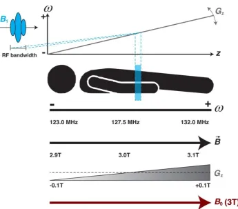
Figure 2.4: Illustration of selective excitation, showing: the static B0 field (shown at 3T); the applied spatially-varying magnetic gradient, Gz; the combined magnetic fields, 𝐵; and the effects on the procession frequency, . The diagram also illustrates the dependence of the thickness of the excited ‘slice’ on the B1 RF bandwidth and the strength of the applied magnetic gradient, Gz. ... 18

Figure 2.5: Schematic representation of the MR scanner hardware (section removed) showing the locations of the shielding and respective Magnet, gradient, and RF coils, as well as the three types of magnetic fields that these coils produces. ... 19

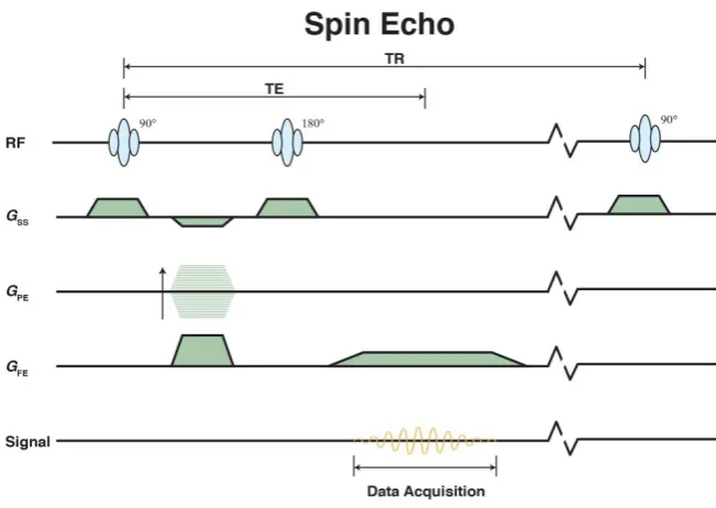
Figure 2.6: Pulse sequence diagram (PSD) for the basic spin echo sequence. Figure illustrates the timing of the B1 radiofrequency (RF) transmit field, as well as the gradients used for slice selection (Gss), phase encoding (GPE), and frequency encoding (GFE). ... 23

Figure 2.7: Pulse sequence diagram (PSD) for the basic gradient echo sequence. Figure illustrates the timing of the B1 radiofrequency (RF) transmit field, as well as the gradients used for slice selection (Gss), phase encoding (GPE), and frequency encoding (GFE). ... 24

Figure 2.8: Pulse sequence diagram (PSD) for the basic spoiled gradient echo sequence. Figure illustrates the timing of the B1 radiofrequency (RF) transmit field, as well as the gradients used for slice selection (Gss), phase encoding (GPE), and frequency encoding (GFE). ... 24

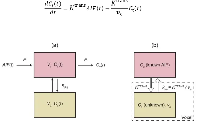
Figure 2.9: (a) Illustration of the prostate gland, showing the peripheral zone (PZ), central zone (CZ), and transition zone (TZ) as well as a schematic representation of the contrast agent exchange process, taking place on the micro-vessel scale. (b) An example bulk signal-time curve (STC). ... 29

Figure 2.10: Signal-time curve (STC) time curve showing examples of phenomenological parameters, namely: wash-in, wash-out, time-to-peak, and integral area under the curve after 60 seconds (IAUC60). ... 30

Figure 2.11: Schematic diagrams showing: (a) the general open two-compartment model and (b) the standard Tofts model. ... 32

Figure 2.12: Example of an arterial input function (AIF). ... 34

input/output configuration, and (b) photographs of the final prostate-mimicking object (left: complete, and right: sectioned) containing the two measurement chambers, with inputs into chambers 1 (red) and 2 (blue) highlighted. ... 45

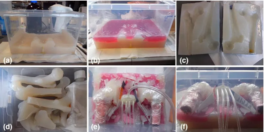
Figure 3.2: (a–f) Photographs showing various stages during construction of the large

anthropomorphic phantom, with: (a) an initial layer of fat TMM; (b) a layer of muscle TMM (red dye used to differentiate from other TMMs); (c) latex moulds used to cast the ‘femur bones’; (d) cast physiologically-shaped components for the phantom, composed of various different TMM materials; (e, f) the prostate mimicking object in situ prior to surrounding TMM being deposited, as well as two ‘femur bones’ composed of bone TMM, and deposition of a heterogeneously distributed fat / muscle layer. ... 46

Figure 3.3: Photograph of the final phantom device. Dimensions: 280(w) x 390(l) x 200(h) mm3. ... 46

Figure 3.4: Schematic diagram of complete pump system (red and blue traces are

representative of the change in flow rate at each pump over time, with the overall flow-rate kept constant) ... 47

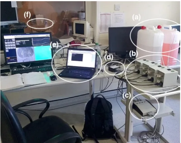
Figure 3.5: Photograph of the phantom system set up in situ in the MR centre. Shown are the (a) the contrast agent reservoirs, (b) the 4-pump system, (c) a custom built control box connecting (d) the analog output module to the pumps, (e) the laptop used to control the phantom system, and (f) the phantom test device in situ at the MR scanner bore. ... 48

Figure 3.6: Schematic diagram of optical imaging system setup used to establish minimum flow rates and ground truth measurements for the CTCs produced by the system. ... 49

Figure 3.7: Example optical calibration curve with the calibration model fit to the data. ... 50

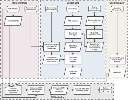
Figure 3.8: Flow diagram illustrating the steps implemented in the analysis of the DCE-MRI and optical data. ... 53

Figure 3.9: Graphs showing: (a) the % root mean square error (%RMSE) values calculated between the programmed and optically-measured CTCs at different flow rates (presented as a percentage of the overall programmed CTCs amplitude); and (b) the programmed and optically-measured ground truth tumour CTCs (optically-measured with 1.5 ml s-1 flow rate). ... 54

Figure 3.10: Graphs showing five repeated measurements of the (a) tumour and (b) healthy CTCs used in this study, using the optical imaging system at 1.5 ml s-1 flow rate. ... 55

Figure 3.11: Axial T1-weighted image of the anthropomorphic phantom with the ‘prostate’ and measurement chambers highlighted. Regions mimicking subcutaneous fat, muscle, and bone are also visable. ... 56

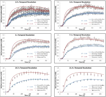
Figure 3.12: Plots presenting tumour and healthy CTCs derived from DCE-MRI data at 1.9 to 21.4 s temporal resolutions, compared with the ground truths derived from optical scanner data. ... 56

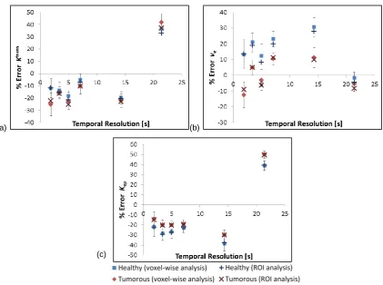
Figure 3.13: Percentage errors in (a) Ktrans, (b) ve, and (c) kep values derived from the DCE-MRI data using the standard Tofts model. Values shown for both a voxel-wise and ROI analysis of the data. Error bars shown for voxel-wise results taken from the standard deviation in the data. ... 57

Figure 4.1: Representative T1-weighted (a) axial and (b) coronal scans of the phantom during peak enhancement within the ‘prostate’ region. The white box in (a) outlines the region shown in (c). (c) Example pharmacokinetic parameter map (Ktrans) showing the ROIs placed within the measurement chambers which were used to measure the ‘healthy’ (ROI 1) and ‘tumour’ (ROI 2) parameter values ... 64

series at the CTC peak (tumour) at each of the temporal resolution (Tres) values tested. SNR values derived from the DCE-MRI data are also presented. (SNR results presented herein should be treated as relative, for the purpose of highlighting relative behavioural trends in the data) ... 65

Figure 4.3: Graphs showing the MR-measured CTCs at different temporal resolution (Tres) values, with error bars derived from the standard deviation across the ROI. The larger error bars for shorter Tres times reflect the decreased SNR in these datasets. Ground truth CTCs are also shown as solid lines. ... 66

Figure 4.4: Correlation plots of the MR-measured versus ground truth CTCs for full 600-second CTC measurements. The diagonal line indicates equality, with divergence from this line

indicating discrepancies between the MR-measured and ground truth values. The CCC values are also shown, along with their 95% confidence intervals. ... 67

Figure 4.5: Percentage errors in wash-in and wash-out parameter values derived from the DCE-MRI data at different temporal resolutions (Tres) using the standard Tofts model. Error bars derived from the standard deviation of the data. ... 68

Figure 4.6: Percentage errors in Ktrans values derived from the DCE-MRI data at different temporal resolutions (Tres) and acquisition durations using the standard Tofts model. Error bars were derived from the standard deviation of the data. ... 68

Figure 4.7: Percentage errors in ve values derived from the DCE-MRI data at different temporal resolutions (Tres) and acquisition durations using the standard Tofts model. Error bars derived from the standard deviation of the data ... 69

Figure 5.1: Graph showing the empirical mathematical formulations for the arterial input function (AIF) as proposed by Weinmann et al. and Parker et al. ... 74

Figure 5.2: (a) Diagram of modified section of the phantom, showing the input tubing set within the imaging volume, with direction of flow indicated. Photographs showing (b) the additional 2 chambers added into the phantom device and (c) the two chambers and tubing in situ in the phantom. ... 80

Figure 5.3: Graph showing the arterial input functions (AIFs) derived from 32 patient DCE-MRI datasets. ... 85

Figure 5.4: Graph showing the population-average arterial input function (AIF), taken as mean of the 32 measured AIFs, with error bars showing standard deviation from the mean, with the Parker model fit also shown. ... 85

Figure 5.5: Graph showing the intrinsic pump response to square wave voltage inputs of varying widths from 5 to 60 s in increments of 5 s. ... 86

Figure 5.6: Graph the normalised pump response curves all transposed to the same temporal starting position. ... 86

Figure 5.7: Graph showing the patient derived population average AIF (blue plot) and the intrinsic pump response to 10 s square wave input (dashed black plot). ... 86

Figure 5.8: Graph showing the patient derived population average AIF (AIFPA; dashed black plot), the empirically-derived input curve required to produce the desired AIF shape (light blue plot), and the resultant optically measured ‘ground truth’ AIF (AIFGT; green data points). ... 87

Figure 5.9: Graph showing the mean patient-data derived AIF, the established ground truth AIF, with the Parker AIF model fit also shown ... 88

representative of reported patient values)... 88

Figure 5.11: Graph showing the MR-measured AIF and tissue contrast contrast-time curves (CTCs) for the non-flip-angle corrected MR data for a single experimental run, with error bars showing the standard deviation across the ROIs. ... 89

Figure 5.12: Graph showing the MR-measured AIF and tissue contrast contrast-time curves (CTCs) for the voxel-wise flip angle corrected data for a single experimental run, with error bars showing the standard deviation across the ROIs. ... 90

Figure 5.13: Graphs showing the mean absolute pharmacokinetic parameter values derived from both the intra- and inter-session datasets without voxel-wise flip-angle correction (VFAC) applied to the data. Black error bars show the intra-session standard deviation from the mean, and the red / blue error bars show the inter-session standard deviation from the mean. ... 92

Figure 5.14: Graphs showing the mean absolute pharmacokinetic parameter values derived from both the intra- and inter-session datasets with voxel-wise flip-angle correction (VFAC) applied to the data. Black error bars show the intra-session standard deviation from the mean, and the red / blue error bars show the inter-session standard deviation from the mean. ... 93

Figure 6.1: Diagram illustrating the 2D golden-angle (111.25) radial ‘stack-of-stars’ k-space sampling scheme which employs golden angle radial sampling in-plane (kx / ky)and Cartesian sampling in the slice direction (kz). ... 100

Figure 6.2: Illustration of Linear Angle and Golden Angle radial MRI data sampling trajectories (k-space units normalised). For linear angle, images are typically reconstructed once full radial coverage has been acquired. However, for Golden angle, an approach wherein images may be reconstructed from differing consecutive numbers of radial profiles of sampled k-space data, can be employed, thereby giving additional flexibility regarding the achievable temporal

resolutions (Tres). (Image adapted from [209]). ... 101

Figure 6.3: Schematic diagram showing the various steps involved in the Coil-by-Coil (CbC) inverse gridding, Parallel Imaging (PI), and PI and Compressed Sensing (PICS) DCE-MRI reconstruction. Numbering corresponds to steps outlined in section 6.2.2. ... 108

Figure 6.4 Images reconstructed with radial sampling densities (RSDs) from 100% to 4.68% using the Coil-by-Coil (CbC) inverse gridding, Parallel Imaging (PI), and PI and Compressed Sensing (PICS) reconstruction methods ... 110

Figure 6.5: Graphs showing the mean absolute pharmacokinetic parameter values derived from both the intra- and inter-session datasets at various radial sampling densities (RSDs) for coil-by-coil (CbC), parallel imaging (PI), and PI with compressed sensing (PICS) image reconstruction methods. Black error bars show the intra-session standard deviation from the mean, and the red / blue error bars show the inter-session standard deviation from the mean. The dashed horizontal lines show the ground truth values in each case. ... 115

Figure A1.1: Photograph of prototype mixing chambers produced using (left) the Form1+

(Formlabs, USA) system and (right) the Eden 250 (Stratasys, USA) system. ... A-1

Figure A1.2: Photograph showing the shielded control box used to connect the 25 way d-sub connection from the analog output module to the four individual pumps (15 way d-sub), as well as control whether the pumps flow-rates were manually set at the driver units or controlled via the output module’s output voltage, shown: (a) with control switches and voltage output connection highlighted; (b) open, showing the internal wiring; and (c) connected to an

oscilloscope via a purpose-built cable for validation of the voltage outputs. ... A-2

Figure A1.3: Schematic diagram showing the shielded control box wiring configuration. ... A-2

Abbreviations

Abbreviation Definition

AD Acquisition Duration

ADC Apparent Diffusion Coefficient

AFI Actual Flip angle Imaging

AIF Arterial Input Function

CA Contrast Agent

CCC Concordance Correlation Coefficient

CS Compressed Sensing

CTC Concentration-Time Curve

DCE Dynamic Contrast Enhanced

DTI Diffusion Tensor Imaging

DWI Diffusion Weighted Imaging

EBRT External Beam Radiotherapy Treatment

EES Extravascular-Extracellular Space

FID Free-induction decay

FOV Field Of View

GA Golden Angle

Gd Gadolinium

GS Gleason Score

ICC Intraclass Correlation Coefficient

LLS Linear Least Squares

MP Multi Parametric

MRI Magnetic Resonance Imaging

MRSI Magnetic Resonance Spectroscopic Imaging

NLS Non-linear Least Squares

NMR Nuclear Magnetic Resonance

NSA Number of Signal Averages

PCa Prostate Cancer

PD Proton Density

PI Parallel Imaging

PICS Parallel Imaging and Compressed Sensing

PK Pharmacokinetic

PSA Prostate Specific Antigen

PSD Pulse Sequence Diagram

RF Radiofrequency

RMSE Root Mean Square Error

ROI Region Of Interest

SNR Signal-to-Noise Ratio

STC Signal-Time curve

TE Echo Time

TMM Tissue Mimicking Material

TR Repetition Time

Tres Temporal Resolution

TRUS Transrectal Ultrasound

List of Symbols

Quantity Definition Unit

 Flip angle 

act Actual flip angle 

set Set flip angle 

set Set flip angle 

AIF Arterial Input Function: Concentration entering the capillary bed on the arterial side

mM*

B1 Rotating radiofrequency magnetic field T

𝐶𝑐 Concentration in the capillary plasma volume mM

𝐶𝑒 Concentration in the extravascular-extracellular space volume mM

𝐶𝑡 Tissue bulk concentration mM

F Perfusion (or flow) of the whole blood per unit mass of tissue ml g-1 min-1#

kep Rate constant min-1

KPS Capillary transfer coefficient min-1

Ktrans Volume transfer coefficient min-1

Mo Equilibrium magnetisation T

Mxy Transverse magnetisation T

Mz Longitudinal magnetisation T

ρ Tissue density g ml-1

P Total permeability of the vessel wall cm min-1

PS Permeability surface area product per unit mass of tissue ml min-1 g-1

r1 Relaxivity of the contrast agent mM

-1 s-1

S Surface area product per unit mass of tissue cm g-1

T1 Longitudinal magnetisation relaxation time ms

T2 Transverse magnetisation relaxation time ms

𝑇2∗ Effective transverse magnetisation relaxation rate ms

TE Echo Time ms

TR Repetition Time ms

Vc Total capillary plasma volume ml

Ve Total extravascular-extracellular space volume ml

Vp Total plasma volume ml

Vt Total tissue volume ml

vc Capillary plasma volume fraction

ve Extravascular-extracellular space volume fraction

vp Plasma volume fraction

*1 mM = 1 mmole L-1

#

List of Tables

Table 3.1: Composition of tissue mimic materials (TMMs) used in construction of

anthropomorphic phantom... 45

Table 3.2: MRI scan parameters, adjusted to achieve temporal resolutions (Tres) from 1.9 s to 21.4 s. ... 52

Table 5.1: The concordance correlation coefficient (CCC) and pecentage root mean square error (%RMSE) results from repeat intra- and inter-session optical experiements. ... 87

Table 5.2: Parker AIF function parameter values for the MR-measured population average AIF (AIFPA) and the optically-measured ground truth AIF (AIFGT) used in this study. ... 88

Table 5.3: Programmed and optically-established ground truth PK parameter, derived by fitting the standard Tofts model using LLS and NLS approaches (± the standard deviation across all 9 experiments) ... 89

Table 5.4: The concordance correlation coefficient (CCC) with 95% confidence intervals (CI) and percentage root mean square error (%RMSE) results from repeat intra- and inter-session DCE-MRI experiments (given with and without voxel-wise flip-angle correction (VFAC). ... 90

Table 5.5: Measured signal-to-noise ratio (SNR) values across the range of temporal resolution (Tres) values used in this study. ... 90

Table 5.6: Absolute maximum % error and % standard deviation (S.D.) in the measurement of pharmacokinetic parameters using the base 1.2 s temporal resolution (Tres) acquisition protocol, with and without voxel-wise flip-angle correction (VFAC). ... 92

Table 5.7: Temporal resolution (Tres) requirements in order to achieve errors  5%, 10%, 15%, and 20% in pharmacokinetic parameter estimates. Data taken from all 9 experimental runs (five intra-session and five inter-session), with voxel-wise flip-angle correction (VFAC) applied. ... 93

Table 6.1: Parameters used in the reconstruction of the DCE-MRI data-sets, along with the reconstruction times. ... 108

Table 6.2 The concordance correlation coefficient (CCC) with 95% confidence intervals (CI) and percentage root mean square error (%RMSE) results from repeat intra- and inter-session DCE-MRI experiments, comparing the fully-sampled (radial sampling density (RSD) = 100%) MR-measured AIF with the ground-truth AIF. Results presented for coil-by-coil (CbC), parallel imaging (PI), and parallel imaging with compressed sensing (PICS) image reconstruction methods. ... 111

Table 6.3: Absolute maximum % error and % standard deviation (S.D.) in the measurement of pharmacokinetic parameters at radial sampling density (RSD) from 100% to 4.68%, using for coil-by-coil (CbC), parallel imaging (PI), and parallel imaging with compressed sensing (PICS) image reconstruction approaches. ... 113

Chapter 1: Introduction

1.1. Context and Motivation

As men age, benign or malignant changes commonly occur in the prostate tissue, with prostate cancer (PCa) being one such a malignant disease. PCa is the second most frequently diagnosed cancer among males worldwide [1] and the second leading cause of cancer death in men [2]. As with most diseases, the early and accurate diagnosis of PCa greatly enhances treatment prognosis. Currently the main method for PCa screening is prostate specific antigen (PSA) testing, with patients who present with elevated PSA results generally sent for an invasive transrectal ultrasound (TRUS) guided biopsy. TRUS biopsies are known to be inaccurate , with data suggesting that up to 30% of tumours are not detected [3], and repeat random biopsies failing to improve tumour detection rates [4-6]. There is thus a need for more accurate and precise, preferably non-invasive, technique for the detection and characterisation of PCa.

PCa [7, 8], studies conducted in 1995 found an improvement in tumour localisation when imaged early after contrast administration [9], as well as an improvement in the

detection of minimal seminal vesicle invasion by tumour tissue [10]. Since then, studies have repeatable shown the potential of DCE-MRI as a possible non-invasive gold standard imaging technique for PCa detection [11], localisation [12, 13], and grading [14, 15].

However, although numerous patient studies over the past twenty-plus years have shown the effectiveness of DCE-MRI for PCa imaging, to data no method has been proposed which allows for a comprehensive validation and quantification of DCE-MRI acquisition, reconstruction, pre-processing, and analysis techniques. This has

hindered this potentially-diagnostically-useful technique’s full adoption for routine clinical use.

In this thesis a phantom test device is presented that essentially provided a ‘model patient’, wherein concentration-time curves (CTCs) were precisely known and controlled, and could be repeatedly produced and measured using DCE-MRI. The device addressed two key limitations of patient-based attempts to quantify the accuracy and precision of DCE-MRI, namely: knowledge of the ground truth contrast agent (CA) CTCs (both tissue and arterial), and repeatability. The device allowed for the absolute accuracy and precision of various DCE methodologies to be quantitatively accessed for the first time

1.2. Dynamic Contrast Enhanced (DCE) MRI for Prostate Cancer Imaging

1.2.1. Tumour Detection

In a 2005 study on men with elevated PSA levels (PSA > 2.5 ng/ml), Hara et al. imaged 90 patients prior to TRUS-biopsy. Of the 90 patients, 57 patients presented with PSA < 10.0 ng ml-1, of which the initial TRUS-biopsy had a detection rate of 36.8% and DCE-MRI was reported as being successful in detecting 92.9% of the clinically significant PCa for the first biopsy session, with a specificity of 96.2%. This study used qualitative analysis of the results; a radiologist manually inspected the DCE data and considered a lesion with an early enhanced peak and immediate wash-out to be PCa [13]. A 2011 study by Tamada et al. on 50 men with PSA values between 4 and 10 ng ml-1 reported sensitivity and specificity of 74% and 80% respectively, backing up the conclusion put forward by Hara et al. that DCE-MRI alone is equivalent or occasionally superior to 6 or 8 core biopsy protocols in the detection of PCa, even with PSA levels less than 10 ng ml-1[16].

In a clinical setting, DCE-MRI is usually performed as part of a multi parametric (MP) MRI imaging protocol, combining various MRI techniques, such as: T2-weighted imaging, DCE, diffusion weighted imaging (DWI), diffusion tensor imaging (DTI), and MR spectroscopic imaging (MRSI), into a single protocol. The inclusion of DCE in this MP approach has shown great promise for PCa imaging, as discussed in a brief review of the literature below.

Kozlowski et al., in a 2006 study on 14 patients, correlated multiple DCE-MRI parameters with histology and found that Ktrans, onset time, mean gradient and

maximum enhancement of the contrast time-intensity curve (CTC) showed significant differences between tumour and normal tissue, with overall sensitivity of 59% and specificity of 74% when using DCE-MRI alone. In cancerous prostate tissue the normal glandular architecture is replaced by aggregated cancer cells and fibrotic stroma, which inhibits the movement of water macromolecules, resulting in restricted diffusion and a reduction in the apparent diffusion coefficient (ADC) values, which can be measured using DWI-MRI. Kozlowski also investigated the use of DCE in

combining DCE with DTI for the detection of PCa in the peripheral zone. The study compared the MR images to sextant biopsy results by drawing regions of interest according to the biopsy zones. They found significant difference in the ADC, Ktrans, and kepvaluesbetween tumorous and non-tumorous sextants. The area under the curve for

the combination of DCE and DTI-MRI was also found to be greater than for either DCE (0.93 vs. 0.84) or DTI (0.93 vs. 0.86) alone, suggesting better diagnostic performance when these techniques are used conjointly [19].

Several other studies [4, 20, 21] have also investigated the additional diagnostic value of combining MRSI and DCE-MRI, with reported sensitivities of 29-100%, specificities of 48-96%, and accuracies of 67-91%. MRSI detects abnormal metabolism rather than abnormal anatomy, differentiating tumorous from healthy prostate tissue by differences in the choline-creatine-to-citrate ratio [21]. In a 2010 study on 68 patients, Portalez et al. compared T2-weighted, DCE, MRSI, and DWI techniques in guided repeat biopsies. They reported that out of the four techniques, DCE had the lowest sensitivity for PCa detection of 29%, it did however have high specificity (93%) and accuracy (86%). As noted by the authors, their DCE protocol had too low a temporal resolution (Tres = 13 s) to accurately apply quantitative pharmacokinetic (PK) modelling to the data [22], instead a qualitative approach was employed, which looked at maximum enhancement, wash-in rate, time-to-peak, and wash-out wash-information, which may have led to such low sensitivity [20]. The importance of adequate Tres is well demonstrated by another larger study performed the same year by Panebianco et al. on 150 patients. This study was conducted in a similar manor to the Portalez study, but with the DCE data being acquired at a higher temporal resolution of 3s. The Panebianco study reported a sensitivity of 76.5%, and specificity of 89.5% for DCE alone, and sensitivity of 93.5% and specificity of 90.7% for MRSI and DCE combined, with a reported accuracy of 90.9% in detecting prostate carcinoma [21]. A 2013 study by Perdonā et al. on 106 patients reported diagnostic accuracy for DCE combined with MRSI of 85%, with sensitivity of 71% and specificity of 48% for PCa detection [23].

1.2.2. Accessing Tumour Aggressiveness

phenomenological and PK analysis of high Tres (3 s) DCE data to access the

aggressiveness of PCa in the peripheral zone, with wash-in, Ktrans, and kep offering the

best possibility to discriminate low-grade, intermediate-grade, and high-grade PCa [14]. Conversely, studies by Padhani et al. [24] and Ota et al. [25] found no significant

correlation between DCE parameters and GS. Padhani did however report weak correlation between local tumour stage and both tumour vascular permeability, and maximum tumour Gd concentration [24], and Ota found that both mean blood vessel count, and mean vessel area fraction, had significant correlation with kep[25].

1.2.3. Treatment Monitoring and Detection of Recurrence

Approximately 30% of patients diagnosed with PCa will undergo external beam radiotherapy treatment (EBRT) as their initial treatment [26]. It has been reported that 15% of low-risk and 67% of high-risk patients will experience an increase in PSA levels within 5 years of EBRT [27]. An increase in PSA level post-treatment (over a threshold of 0.2 ng ml-1[28]) can indicate a relapse of PCa, however PSA levels may fluctuate after therapy, and an increase in PSA level does not necessarily indicate recurrence [29, 30]_{. In a 2013 meta-analysis of nine previous studies of PCa recurrence detection after} EBRT, Wu et al. reported pooled sensitivity of 82% and specificity of 74% using DCE alone [31]. The addition of DCE-MRI has also been shown to significantly increase sensitivity for the detection of recurrent PCa after EBRT, compared with T2-weighted imaging alone; with one study reporting increases in sensitivity from 38% to 72%, and specificities from 80% to 85% [32]. Kara et al. reported greater sensitivity, specificity, and accuracy using DCE (93%, 100%, and 95% respectively), when compared to TRUS biopsy (53.3%, 60% and 55% respectively), concluding that TRUS biopsy without the use of additional imaging or biochemical modalities was not sufficient for the detection of PCa recurrence [33]. A study by Moman et al. also highlighted the potential use DCE in the planning of focal salvage treatment, which could reduce the adverse effects of radiotherapy [34].

al. on 47 patients highlighted the potential use of DCE in the detection of recurrence of PCa after radical prostatectomy, reporting a high degree of accuracy in the detection of sub-centimetre local recurrences within the post-prostatectomy bed. They used a spatial resolution of 3mm and reported good sensitivity in detecting local recurrences greater than 5mm [35]. Similarly, a study by Cirillo et al. demonstrated an increase in sensitivity from 61% to 84% and specificity from 82% to 89%, with the inclusion of DCE, compared with T2-weighted imaging alone, in the detection of PCa recurrence post-prostatectomy [36].

Another method used in the treatment of PCa is high-intensity focused ultrasound ablation (HIFU), which causes coagulation necrosis in the targeted tissue by converting mechanical energy into heat and generating a cavitation effect. In a 2008 study, Kim et al. compared DCE-MRI to T2-weighted combined with DWI and found higher average sensitivity for DCE (84%) compared to T2-weighted with DTI (67%), but higher

specificity and accuracy using T2-weighted with DTI (76% and 73% respectively), compared to DCE (66% and 72% respectively) [37]. Rouviēre et al. investigated the use of T2-weighted and DCE-MRI in guiding targeted biopsies after HIFU treatment. They found that targeted biopsies detected more cancers than routine biopsies (36 vs. 27 patients), implying that MRI combining T2-weighted and DCE images could be a promising method for post-HIFU guided biopsy [38].

.

1.3. Aims and Objectives of the Thesis

The main aim of this thesis was to develop a model system capable of producing highly-repeatable, precisely-known, physiologically-relevant CTCs and arterial input function (AIF) curves within an anthropomorphic environment for repeated

values against precisely-known ground truths. This was all done with the overall goal of informing future phantom and patient studies, ultimately with the intention of

improving the PCa diagnostic capabilities of DCE-MRI, and potentially leading to a wider acceptance of the technique for use in routine clinical examinations.

The specific objectives of the thesis can be summarised as follows:

1. Design and build a physical dynamic phantom test device for the validation and development of DCE-MRI techniques. The device must be:

 able to reproducibly generate arbitrarily-shaped (programmable) and precisely-known CTCs which mimic those observed in healthy and tumorous prostate tissue, as well as other physiological curve shapes, such as the arterial input function (AIF)

 anthropomorphic in nature, mimicking the male pelvic-region in terms of size, image complexity, and sparsity; to allow for comprehensive testing of DCE-MRI techniques, provide patient-relevant results, and allow for easy clinical translation of protocols developed on the device

 capable of producing MR-measurable CTCs, i.e. produced in a region large enough to accommodate several imaging voxels, while avoiding any partial-volume issues

 capable of producing CTCs at low flow rates, to avoid flow related artefacts and minimise CA usage

 able to produce two distinct curves simultaneously, to allow for different tissue CTCs (‘healthy’ and ‘tumour’) and an AIF to be measured

simultaneously (for the purposes of performing PK modelling on the data)

2. Fully validate the phantom test device, as well as accurately and precisely establish ground truth values for the system using a modality other than MRI. This validation approach had to provide:

 highly-precise, temporally-stable, high-spatiotemporal resolution measurements of the exact CA concentration-change over time  measurements which were directly comparable with the DCE-MRI

results

parameters and methodologies related to the acquisition, reconstruction, pre-processing, and analysis, on the accuracy and precision of DCE

measurements, namely:

 temporal resolution (Tres): the temporal spacing between successive DCE images

 acquisition duration (AD): the length of time that the CTCs and AIF are sampled for

 voxel-wise flip-angle correction (VFAC): in order to compensate for non-uniformity in the B1+-field

 PK model fitting regime: non-linear verses linear fitting approaches  k-space acquisition trajectory: the order and manner in which the MR

frequency-encoded data are sampled

 under-sampling k-space: in order to achieve faster imaging times  reconstruction methodologies: using coil-by-coil (CbC) inverse gridding,

parallel imaging (PI), and PI combined with compressed sensing (PICS) approaches

1.4. Thesis Overview

This thesis is divided into seven main chapters, with each chapter thematically related, and subsequent chapters being informed by the results of the preceding ones. The outline of the thesis reads as follows:

Chapter 2: Background

The subject matter of this chapter formed the basis of the following:

Conference Proceeding

Knight, S.P., Meaney J.F., Fagan A.J., A review of dynamic contrast enhanced MRI for the

diagnosis of prostate cancer. [poster] Irish Association of Physicists in Medicine (IAPM) annual

scientific conference, 22nd February, 2014, Dublin, Ireland. Phys Medica 30(6): 721 (2014) DOI:

10.1016/j.ejmp.2014.06.024

Chapter 3: Design, fabrications, and validation of a novel anthropomorphic

DCE-MRI prostate phantom test device

As previously stated, one of the main factors currently limiting the implementation of DCE-MRI as a truly quantitative technique is the lack of a comprehensive validation method, stemming from a lack of knowledge of the ground-truth conditions within the patient or object being scanned. In this initial phase of the project a novel

anthropomorphic phantom test device was designed and built. The device allowed for precisely and accurately known ground truth CTCs to be repeatedly generated within an environment with mimicked that of a patient, and presented to the MRI scanner for measurement, thereby allowing for a quantitative assessment of the accuracy and precision of a particular DCE-MRI approach. CTC derived from prior patient prostate data were produced by means of a custom-built 4-pump flow system. The ground truths for the system was determined using an MRI-independent, highly-precise, custom-built optical imaging system. Preliminary DCE-MRI data for the phantom device is also presented in this chapter, demonstrating the operation of the device.

The subject matter of this chapter formed the basis of the following:

Journal Publication

Knight, S.P., Browne, J. E., Meaney J.F., Smith, D.S., Fagan A.J., A novel anthropomorphic flow

phantom for the quantitative evaluation of prostate DCE-MRI acquisition techniques. Phys Med

Biol, 2016. 61(2): p. 7468-7483 (2016) DOI: 10.1088/0031-9155/61/20/7466

Conference Proceedings

Knight, S.P., Browne, J. E., Meaney J.F., Smith, D.S., Fagan A.J. A Novel Prostate DCE-MRI

Flow Phantom for the Quantitative Evaluation of Pharmacokinetic Parameters. [oral] International

Knight, S.P., Browne, J. E., Meaney J.F., Smith, D.S., Fagan A.J., Error quantification in

pharmacokinetic parameters derived from DCE-MRI data using a novel anthropomorphic dynamic

prostate phantom. [oral] Irish Association of Physicists in Medicine (IAPM) annual scientific

conference, 2nd April, 2016, Waterford, Ireland. Phys Medica 32(7): 949 (2016) DOI:

10.1016/j.ejmp.2016.05.012

Knight, S.P., Browne, J. E., Meaney J.F., Fagan A.J. A novel flow phantom for the quantitative

evaluation of prostate DCE-MRI techniques. [oral] European Society for Magnetic Resonance in Medicine and Biology (ESMRMB) annual scientific conference, 1st – 3rd October, 2015,

Edinburgh, Scotland. Magn Reson Mater Phy 28(Suppl 1): p. S383-384. (2015) DOI:

10.1007/s10334-015-0489-0

Knight, S.P., Meaney J.F., Fagan A.J., A flow phantom for the quantitative validation of DCE-MRI

techniques. [oral] Irish Association of Physicists in Medicine (IAPM) annual scientific conference,

27th February 2015, Dublin, Ireland. Phys Medica 32(2): 417 (2016) DOI:

10.1016/j.ejmp.2015.07.016

Knight, S.P., Meaney J.F., Fagan A.J., Rapid prototyping: Offering new opportunities in phantom

design and construction. [poster] Irish Association of Physicists in Medicine (IAPM) annual

scientific conference, 27th February 2015, Dublin, Ireland. Phys Medica 32(2): 427 (2016) DOI:

10.1016/j.ejmp.2015.07.053

Chapter 4: Effects of acquisition duration and temporal resolution on the

accuracy of prostate tissue concentration-time curve measurement and derived

phenomenological and pharmacokinetic parameter values

This chapter utilises the phantom test device presented in Chapter 3 to investigate the effect of the Tres and AD on the measurement accuracy of tissue CTCs, and derived phenomenological and pharmacokinetic parameter values. The Tres and AD values tested were representative of the wide-range of values reported in the literature to date for DCE studies in the prostate (Tres = 2 - 24.4 s and AD = 30 – 600 s), and the effects on the measurement accuracy of the wash-in, wash-out, Ktrans, and ve parameters were quantified. The hypothesis under investigation was whether measurement

The subject matter of this chapter formed the basis of the following:

Journal Publication

Knight, S.P., Browne, J. E., Meaney J.F., Fagan A.J., Quantitative effects of acquisition duration

and temporal resolution on the measurement accuracy of prostate dynamic contrast enhanced

MRI data. Magn Reson Mater Phy,. 30(5): p. 461-471 (2017) DOI: 10.1007/s10334-017-0619-y

Conference Proceedings

Knight, S.P., Browne, J. E., Meaney J.F., Fagan A.J. Quantitative evaluation of the effect of

temporal resolution and acquisition duration on the accuracy of DCE-MRI measurements in a

prostate phantom. [poster]International Society for Magnetic Resonance in Medicine (ISMRM)

25th Annual Scientific Meeting and Exhibition, 22nd – 27th April, 2017, Honolulu, Hawaii, USA.

Proc. Intl. Soc. Mag. Reson. Med. 25: 2890, (2017)

Knight, S.P., Browne, J. E., Meaney J.F., Fagan A.J. Effects of sampling frequency on the

accuracy of phenomenological and pharmacokinetic parameters derived from dynamic contrast

enhanced MRI data. [oral] Irish Association of Physicists in Medicine (IAPM) Annual Scientific

Conference, 25th March, 2017, Dublin, Ireland

Knight, S.P., Browne, J. E., Meaney J.F., Fagan A.J. Quantitative evaluation of the effects of

dynamic contrast enhance MRI acquisition parameters on the accuracy of derived prostate

cancer biomarkers. [poster] Irish Association for Cancer Research (IACR) annual scientific conference, 23rd – 24th February, 2017, Kilkenny, Ireland

Knight, S.P., Browne, J. E., Meaney J.F., Fagan A.J. A novel anthropomorphic phantom test

device for the validation and development of dynamic contrast enhanced MRI protocols. [oral] Bioengineering in Ireland²³, 20th – 21st January, 2017, Belfast, Northern Ireland

Knight, S.P., Browne, J. E., Meaney J.F., Fagan A.J. A novel anthropomorphic test device for the

assessment of dynamic contrast enhanced MRI of prostate cancer. [poster] The 10th International Cancer Conference, 17th – 18th October, 2016, Dublin, Ireland

Knight, S.P., Browne, J. E., Meaney J.F., Fagan A.J. Effect of temporal resolution and sampling

duration on pharmacokinetic parameters derived from prostate DCE-MRI data: a quantitative

phantom study. [oral] European Society for Magnetic Resonance in Medicine and Biology (ESMRMB) annual scientific conference, 29th September – 1st October, 2016, Vienna, Austria.

Magn Reson Mater Phy 29(Suppl 1): p. S261 (2016). DOI:10.1007/s10334-016-0570-3

Chapter 5: Effects of temporal resolution, voxel-wise flip-angle correction, and

model-fitting regime on the accuracy and precision of arterial and

parameter values

Accurate and precise measurement of the AIF is essential for PK modelling to be accurately performed using certain PK models, such as the widely-used standard Tofts model. Although a number of population-average formations of the AIF have been proposed, acquiring a patient-specific AIF remains the only method that allows for truly quantitative patient-specific PK parameters to be derived. However the measurement of the AIF has proved challenging due to several confounding factors, such as the use of an inappropriately-long Tres in the acquisition sequence and non-uniformities in the B1+-field. The aim of this phase of the project was to use the anthropomorphic

phantom test device presented in Chapter 3 to perform a quantitative investigation into the effects of Tres and B1+-field non-uniformities on the accuracy of AIF (and tissue CTC) measurements. The protocol under investigation used a full-sampled, standard Cartesian k-space acquisition trajectory. The ground truth AIF used in this chapter was based on a population-average derived from 32 high-Tres prostate patient datasets, the data from which is also presented. MR-measured tissue CTCs, AIFs, and derived PK parameters, taken from five intra-session and five inter-session phantom experiments (each measuring a ‘healthy’ and ‘tumour’ CTC simultaneously with the ground truth AIF), were compared with precisely-known ground truth values and measurement errors were calculated. Additionally, the data was fit using both non-linear, and more recently proposed linear interpretations of the standard Tofts model, and the

performance of both modelling approaches was accessed.

Chapter 6: Effect of golden-angle radial k-space under-sampling and image

reconstruction methodology on DCE-MRI accuracy and precision

Rapid imaging techniques, such as PI and CS, offer the prospect of greatly reducing imaging times with MRI, thereby vastly improving the Tres for DCE-MRI, and possibly leading to more accurate characterisation of tissue CTCs and AIF, and by extension the derived quantitative PK parameters. However, as was the case for DCE-MRI in general, the lack of a quantitative method for testing and validating these techniques in vivo has meant that the actual effect of using PI and CS on the absolute accuracy and precision of DCE measurements has remained unknown to date.

sampling trajectory, with data reconstructed using three approaches, namely: CbC inverse gridding, PI, and PICS. The fidelity of tissue CTC and AIF curve-shape measurements, as well as the accuracy and precision of the derived PK parameters, were quantified for each reconstruction approach, at a range of different under-sampling factors from 5% to fully-sampled, with all results compared against the precisely-known ground-truth values. As with the preceding chapter,

MR-measurements were taken from five intra-session and five inter-session phantom experiments (each measuring a ‘healthy’ and ‘tumour’ CTC simultaneously with the ground truth AIF). The results from this chapter were also compared with the results of the preceding chapter, which was performed using similar methodologies, but using a fully-sampled Cartesian k-space sampling trajectory.

Chapter 7: Conclusions

Chapter 2: Background

2.1. Magnetic Resonance Imaging

MRI is a non-ionizing medical imaging technique which is used to non-invasively investigate the structure and function of living tissues. The concept was first proposed 1972 by Lauterbur, and the following year the first two-dimensional (2D) images were published [39, 40]. In 1976 and 1977 Mansfield introduced two new techniques which allowed for faster imaging [41, 42], and in 1980 Edelstein and Hutchison introduced the first practical implementation of 2D Fourier transformed MR imaging, dubbed ‘spin warp’ at the time [43]_{. Since then, the field of MRI has grown exponentially, with multiple} different MR imaging techniques proposed for use in many different physiological locations, each designed to measure different specific tissue properties or functional information. These developments allow currently for the production of high-quality diagnostic images using MRI, for interpretation by a trained eye. However more recently there has been a drive towards developing imaging techniques which provide quantitative information about patient-specific physiology, which should allow for more rapid, accurate, and specific diagnosis, as well as easier comparison between

2.1.1. Nuclear Magnetic Resonance Physics

Magnetisation and Precession

The nuclear magnetic resonance (NMR) phenomenon is quantum mechanical in nature, however at the macro scale it can be practically described using classical mechanics. In this Chapter a classical interpretation is presented.

Figure 2.1: Schematic representation showing the rotation of the magnetic moment at the nucleus in a non-ferromagnetic material, along with a bar magnet illustrating magnetic-field line.

NMR can be conceptualised by thinking of each nucleus in a non-ferromagnetic material as a small independent bar-magnet, rotating around an axis located between its magnetic poles, as illustrated in Figure 2.1. In the absence of an external magnetic field the orientations of each nucleus’s magnetic moment is random with respect to one another, as shown in Figure 2.2 (a). If an external magnetic field is applied, B0, a portion of the nuclei magnetic moments will align parallel with the field, others will align antiparallel, while some will remain misaligned due to Brownian motion, as shown in Figure 2.2 (b); producing a small net magnetic moment across the sample, Mz (the longitudinal direction of the B0 field is conventionally designated as the z-axis).

Figure 2.2: (a) Schematic representation of the random orientation of magnetic moments of a group of nuclei in the absence of an externally-applied magnetic field; the vector sum of these magnetic moments

will be practically zero. (b) Effect of applying a strong magnetic field, B0, on the magnetic moments of a

group of nuclei; some of the magnetic moments will be aligned parallel or antiparallel with the applied magnetic field, with a bias toward aligning parallel with the applied field causing a non-zero net magnetic moment for the sample. (Generally speaking the majority of alignments in a sample are due to Brownian

In 1946 the NMR phenomenon was mathematically described by Felix Bloch, in what is now commonly referred to as the Bloch equation [44], given as:

𝜕𝑀⃗⃗

𝜕𝑡 = 𝑀⃗⃗ x 𝜔0−

𝑀_𝑥𝑖̂ + 𝑀_𝑦𝑗̂

𝑇₂ −

(𝑀𝑧− 𝑀0)𝑘̂

𝑇₁ , [2.1]

where: 𝑀⃗⃗ is the magnetic moment of a volume, with 𝑀⃗⃗ = (Mx, My, Mx)T; M0 is the magnitude of the longitudinal net magnetisation at thermal equilibrium; T1 and T2 are time constants specific to the material being imaged (discussed later in this section); 𝑖̂,

𝑗̂, and 𝑘̂ are unit vectors in the x, y, and z direction respectively; and 𝜔₀ is the angular frequency of procession, known as the Larmor frequency (first described by the Irish physicist, Joseph Larmor), and given as:

𝜔₀= 𝛾𝐵⃗ , [2.2]

where 𝛾 is the gyromagnetic ratio (in MHz T-1) and 𝐵⃗ is the strength of the applied magnetic field (in T).

Magnetic resonance

Magnetic resonance (MR) occurs when a radiofrequency (RF) pulse, B1, is applied orthogonal to the B0 field at the Larmor frequency. If we visualise this using a frame of reference rotating at the Larmor frequency [45], this causes M0 to tilt away from B0, and it forms a magnetisation component on the transverse plane (Mxy), as illustrated in Figure 2.3. The precession of the Mxy component induces a current, which when amplified can be detected, and this is called the NMR signal or free-induction decay (FID). If a B1 pulse is applied in the presence of a uniform B0 field then a signal is induced inside everything that receives the RF power, this is called non-selective excitation.

Selective Excitation

processing at that frequency, and hence a volume, or ‘slice’, can be selected in the subject. The thickness of the volume is dictated by the RF bandwidth and strength of the applied magnetic gradients used, also illustrated in Figure 2.4 Selective excitation allows for the imaging field of view to be reduced, and thereby the acquisition time to also be reduced.

Figure 2.3: (a) Schematic representation of the precession of an isolated magnetic moment, , in a static magnetic field B0 (static frame of reference). (b) The net magnetisation, M0, in the equilibrium state, and (b)

in the presence of an RF pulse (B1) where the spins are tipped toward the xy-plane, producing

magnetisation components, Mz and Mxy (frame of reference rotating at the Larmor frequency)

Relaxation

During the applied RF pulse the system is in an excited state, however once the RF is stopped the spin system return back to an equilibrium state, through a process called relaxation. There are two mechanisms by which it does this: longitudinal relaxation of the Mz component and transverse relaxation of the Mxy component.

Longitudinal relaxation is related to how quickly the net magnetisation returns to thermal equilibrium by means of the nuclear spins exchanging energy with their surroundings (known as the lattice). It is described by the – (Mz – M0) 𝑘̂ / T1 term in Equation [2.1]. Assuming 𝐵⃗ is entirely in the z direction, Equation [2.1] simplifies to:

𝜕𝑀_𝑧

𝜕𝑡 = −

(𝑀_𝑧− 𝑀₀)𝑘̂

𝑇₁ , [2.3]

the solution to which is:

𝑀_𝑧(𝑡) = 𝑀₀+ (𝑀_𝑧𝑖 _{− 𝑀}

0)exp (−

𝑡

Figure 2.4: Illustration of selective excitation, showing: the static B0 field (shown at 3T); the applied

spatially-varying magnetic gradient, Gz; the combined magnetic fields, 𝐵⃗ ; and the effects on the procession

frequency, . The diagram also illustrates the dependence of the thickness of the excited ‘slice’ on the B1

RF bandwidth and the strength of the applied magnetic gradient, Gz.

where t is the time relative to the initial magnetisation and 𝑀_𝑧𝑖 is the initial longitudinal magnetisation. This longitudinal relaxation of the Mz component (spin-lattice relaxation) is characterised by the time constant T1.

The second mechanism, transverse relaxation (spin-spin relaxation), does not involve an exchange of energy with the lattice, but rather relates to a loss of phase coherence between spins in the transverse plane. It is characterised by the time constant T2, and is described by the term – (Mx𝑖̂ – My𝑗̂) / T2 term in Equation [2.1]. Only considering this term, the Bloch equation (Equation [2.1]) becomes:

𝜕𝑀⃗⃗

𝜕𝑡 = −

𝑀_𝑥𝑖̂ + 𝑀_𝑦𝑗̂

𝑇₂ , [2.5]

𝑀⃗⃗ _𝑥𝑦(𝑡) = 𝑀⃗⃗ _𝑥𝑦𝑖 _{exp (−} 𝑡

𝑇₂), [2.6]

where 𝑀⃗⃗ _𝑥𝑦= 𝑀_𝑥𝑖̂ + 𝑀_𝑦𝑗̂ , and 𝑀⃗⃗ _𝑥𝑦𝑖 is the initial magnetisation in the transverse plane at t = 0. In practice the 𝑇₂∗ time constant is often reported, and this takes into account the both the effects of T2 decay and magnetic-field non-uniformity.

2.1.2. Hardware

In this section the main hardware components of an MR imaging system will be

introduced. The scanner manipulates the magnetisation of a sample though the use of three types of magnetic fields, namely the static B0 field, the RF B1 field, and the linear magnetic field gradients, Gx, Gy, and Gz. as illustrated in Figure 2.5.

The Static Magnetic Field (B

)

Generally the static longitudinal magnetic B0 field is generated in a clinical scanner using a superconducting solenoid electromagnet, which allows for a homogenous field to be produced along the axis of the scanner bore. The field strength of clinical

scanners typically ranges from 0.3T to 7T (as of 2017); the stronger the magnetic field, the larger the partial alignment of nuclei along the direction of B, and hence the larger the longitudinal magnetisation in the sample with correspondingly higher signal to noise ratio (SNR).

Figure 2.5: Schematic representation of the MR scanner hardware (section removed) showing the locations of the shielding and respective Magnet, gradient, and RF coils, as well as the three types of

The Radio Frequency Field (B

)

The transverse RF B1 field is produced using a specialised coil that is tuned to the Larmor frequency, with a typically body coil produces a field strength  1.6 x 10-5

T. The B1-transmit field, generally given as B1+, is used to excite the magnetisation from an equilibrium state by perturbing, or tipping, the magnetisation from a longitudinal direction to the transverse plane, as previously described. The amount by which the magnetisation is perturbed is given as the flip angle, and is dictated by the amount of RF energy supplied to the subject.

The Linear Magnetic Field Gradients (G

, G

, and G

)

Spatial information, which is used in image formation, is generated through the application of three additional spatially-varying magnetic fields. Three gradient coils are used, Gx, Gy and Gz, to create three linear gradients oriented orthogonal to each other, producing variations in the longitudinal magnetic field strength as a function of spatial position. This causes the resonance frequency of the magnetisation to likewise vary proportionally with the gradient fields, and this variation is used to resolve the resonance signal spatial distribution.

2.1.3. MR Image Formation

k-Space Trajectory

The spatial information that the magnetic gradients of an MR system provides is acquired encoded in the time-domain, and this time-domain is known as k-space (sometimes also referred to as Fourier space). The order in which the k-space data is acquired is known as the trajectory. One way to acquire k-space is to scan it line-by-line in a Cartesian fashion. Data sampled this way can be reconstructed into an image fast and reliably using the inverse fast Fourier transform (iFFT). Its fast and simple implementation, coupled with the fact that this method of acquisition and reconstruction has proven robust to systemic errors, with remaining artefacts being well documented and understood, has meant that Cartesian k-space sampling is currently the mostly widely used approach for clinical imaging.