GILE: A Generalized Input Label Embedding for Text Classification

GILE: A Generalized Input-Label Embedding for Text Classification

Nikolaos Pappas James Henderson

Idiap Research Institute, Martigny 1920, Switzerland

{nikolaos.pappas,[email protected]}

Abstract

Neural text classification models typically treat output labels as categorical variables that lack description and semantics. This forces their parametrization to be dependent on the label set size, and, hence, they are unable to scale to large label sets and generalize to unseen ones. Existing joint input-label text models overcome these issues by exploiting label descriptions, but they are unable to capture complex label relationships, have rigid parametrization, and their gains on unseen labels happen often at the expense of weak performance on the labels seen during training. In this paper, we propose a new input-label model that generalizes over previous such models, addresses their limitations, and does not compromise performance on seen labels. The model consists of a joint nonlinear input-label embedding with controllable capacity and a joint-space-dependent classification unit that is trained with cross-entropy loss to opti-mize classification performance. We evaluate models on full-resource and low- or zero-resource text classification of multilingual news and biomedical text with a large label set. Our model outperforms monolingual and multilingual models that do not leverage label semantics and previous joint input-label space models in both scenarios.

1 Introduction

Text classification is a fundamental NLP task with numerous real-world applications such as topic recognition (Tang et al., 2015; Yang et al., 2016), sentiment analysis (Pang and Lee, 2005; Yang et al., 2016), and question answering (Chen et al., 2015; Kumar et al., 2015). Classification

also appears as a sub-task for sequence prediction tasks such as neural machine translation (Cho et al., 2014; Luong et al., 2015) and summarization (Rush et al., 2015). Despite numerous studies, existing models are trained on a fixed label set using k-hot vectors, and therefore treat target labels as mere atomic symbols without any particular structure to the space of labels, ignoring potential linguistic knowledge about the words used to describe the output labels. Given that semantic representations of words have been shown to be useful for representing the input, it is reasonable to expect that they are going to be useful for representing the labels as well.

Previous work has leveraged knowledge from the label texts through a joint input-label space, initially for image classification (Weston et al., 2011; Mensink et al., 2012; Frome et al., 2013; Socher et al., 2013). Such models generalize to labels both seen and unseen during training, and scale well on very large label sets. However, as we explain in Section 2, existing input-label models for text (Yazdani and Henderson, 2015; Nam et al., 2016) have the following limitations: (i) their embedding does not capture complex label relationships due to its bilinear form, (ii) their output layer parametrization is rigid because it depends on the dimensionality of the encoded text and labels, and (iii) they are outperformed on seen labels by classification baselines trained with cross-entropy loss (Frome et al., 2013; Socher et al., 2013).

In this paper, we propose a new joint input-label model that generalizes over previous such models, addresses their limitations, and does not compromise performance on seen labels (see Figure 1). The proposed model is composed of a joint nonlinear input-label embedding with controllable capacity and a joint-space-dependent classification unit which is trained

139

with cross-entropy loss to optimize classification performance.1 _{The need for capturing complex} label relationships is addressed by two nonlinear transformations that have the same target joint space dimensionality. The parametrization of the output layer is not constrained by the dimen-sionality of the input or label encoding, but is instead flexible with a capacity that can be easily controlled by choosing the dimensionality of the joint space. Training is performed with cross-entropy loss, which is a suitable surrogate loss for classification problems, as opposed to a ranking loss such as WARP loss (Weston et al., 2010), which is more suitable for ranking problems.

Evaluation is performed on full-resource and low- or zero-resource scenarios of two text clas-sification tasks, namely, on biomedical semantic indexing (Nam et al., 2016) and on multilingual news classification (Pappas and Popescu-Belis, 2017), against several competitive baselines. In both scenarios, we provide a comprehensive abla-tion analysis that highlights the importance of each model component and the difference with previous embedding formulations when using the same type of architecture and loss function.

Our main contributions are the following:

(i) We identify key theoretical and practical lim-itations of existing joint input-label models.

(ii) We propose a novel joint input-label embed-ding with flexible parametrization that gen-eralizes over the previous such models and addresses their limitations.

(iii) We provide empirical evidence of the supe-riority of our model over monolingual and multilingual models that ignore label se-mantics, and over previous joint input-label models on both seen and unseen labels.

The remainder of this paper is organized as follows. Section 2 provides background knowl-edge and explains limitations of existing models. Section 3 describes the model components, train-ing, and relation to previous formulations. Sec-tion 4 describes our evaluaSec-tion results and analysis, while Section 5 provides an overview of previous work and Section 6 concludes the paper and provides future research directions.

1_{Our code is available at:github.com/idiap/gile.}

2 Background: Neural Text Classification

We are given a collection D = {(xi, yi), i =

1, . . . , N} made of N documents, where each document xi is associated with labels yi = {yij ∈ {0,1} | j = 1, . . . , k}, and k is the

total number of labels. Each document xi = {w11, w12, . . . , wKiT_Ki} is a sequence of words grouped into sentences, withKibeing the number

of sentences in document i and Tj being the

number of words in sentencej. Each labelj has a textual description composed of multiple words, cj = {cj1, cj2, . . . , cjLj | j = 1, . . . , k} with Lj being the number of words in each description. Given the input texts and their associated labels

seen during the training portion of D, our goal is to learn a text classifier that is able to predict labels both in the seen,Ys, or unseen,Yu, label

sets, defined as the sets of unique labels that have been seen or not during training, respectively, and, hence,Y ∩ Yu =∅andY =Ys∪ Yu.2

2.1 Input Text Representation

To encode the input text, we focus on hierar-chical attention networks (HANs), which are competitive for monolingual (Yang et al., 2016) and multilingual text classification (Pappas and Popescu-Belis, 2017). The model takes as input a document x and outputs a document vector h. The input words and label words are represented by vectors in IRd from the same3 embeddings E ∈IR|V|×d, whereV is the vocabulary anddis the embedding dimension; E can be pre-trained or learned jointly with the rest of the model. The model has two levels of abstraction, word and sentence. The word level is made of an encoder network gw and an attention network aw, while

the sentence level similarly includes an encoder and an attention network.

Encoders. The function gw encodes the

se-quence of input words {wit | t = 1, . . . , Ti} for

each sentenceiof the document, noted as:

h(_wit) =gw(wit), t∈[1, Ti] (1)

2_{Note that depending on the number of labels per}

docu-ment the problem can be a multi-label or multi-class problem.

3_{This statement holds true for multilingual}

and at the sentence level, after combining the intermediate word vectors{h(wit) |t = 1, . . . , Ti}

to a sentence vectorsi ∈IRdw (see below), where

dw is the dimension of the word encoder, the

function gs encodes the sequence of sentence

vectors{si|i= 1, . . . , K}, noted ash

(i)

s . Thegw

andgsfunctions can be any feed-forward (DENSE) or recurrent networks, for example, GRU (Cho et al., 2014).

Attention. Theαwandαsattention mechanisms,

which estimate the importance of each hidden state vector, are used to obtain the sentence si

and document representationh, respectively. The sentence vector is thus calculated as follows:

si = Ti

X

t=1

α(_wit)h(_wit) =

Ti

X

t=1

exp(v>_ituw) P

jexp(vij>uw)

h(_wit)

(2)

where vit = fw(h

(it)

w ) is a fully connected

net-work withWw parameters. The document vector

h ∈ IRdh_{, where d}

h is the dimension of the

sen-tence encoder, is calculated similarly, by replacing uit withvi =fs(h

(i)

s ) which is a fully connected

network with Ws parameters, and uw with us,

which are parameters of the attention functions.

2.2 Label Text Representation

To encode the label text we use an encoder function that takes as input a label description cj and outputs a label vector ej ∈ IRdc ∀j =

1, . . . ,k. For efficiency reasons, we use a simple, parameter-free function to compute ej, namely,

the average of word vectors which describe label j, namely,ej = _L1_j

PLj

t=1cjt, and hence dc = d

in this case. By stacking all these label vectors into a matrix, we obtain the label embedding

E ∈ IR|Y|×d. In principle, we could also use the same encoder functions as the ones for input text, but this would increase the computation significantly; hence, we keep this direction as future work.

2.3 Output Layer Parametrizations

2.3.1 Typical Linear Unit

The most typical output layer consists of a linear unit with a weight matrix W ∈ IRdh×|Y| _{and a} bias vector b ∈ IR|Y| followed by a softmax or sigmoid activation function. Given the encoder’s hidden representation h with dimension size dh,

the probability distribution of outputygiven input xis proportional to the following quantity:

p(y|x)∝exp(W>h+b) (3)

The parameters inW can be learned separately or be tied with the parameters of the embeddingE by settingW =ET if the input dimension ofW is restricted to be the same as that of the embedding E (d = dh) and each label is represented by a

single word description (i.e., whenY corresponds toV andE =E). In the latter case, Equation (3) becomes:

p(y|x)∝exp(Eh+b) (4)

Either way, the parameters of such models are typically learned with cross-entropy loss, which is suitable for classification problems. However, in both cases they cannot be applied to labels that are not seen during training, because each label has learned parameters which are specific to that label, so the parameters for unseen labels cannot be learned. We now turn our focus to a class of models that can handle unseen labels.

2.3.2 Bilinear Input-Label Unit

Joint input–output embedding models can gen-eralize from seen to unseen labels because the parameters of the label encoder are shared. The previously proposed joint input–output embed-ding models by Yazdani and Henderson (2015) and Nam et al. (2016) are based on the following bilinear ranking functionf(·):

f(x, y) =EWh (5)

where E ∈ IR|Y|×d is the label embedding and

W ∈ IRd×dh _{is the bilinear embedding. This} function allows one to define the rank of a given labelywith respect toxand is trained using hinge loss to rank positive labels higher than negative ones. But note that the use of this ranking loss means that they do not model the conditional probability, as do the traditional models above.

would include a nonlinear transformationσ(·), for example, with either:

(a) σ(EW)

| {z }

Label structure

h or (b) Eσ(Wh)

| {z }

Input structure (6)

Secondly, it is hard to control their output layer capacity because of their bilinear form, which uses a matrix of parameters (W) whose size is bounded by the dimensionalities of the label embedding and the text encoding. Thirdly, their loss function optimizes ranking instead of clas-sification performance and thus treats the ground-truth as a ranked list when in reality it consists of one or more independent labels.

Summary. We hypothesize that these are the

reasons why these models do not yet perform well on seen labels compared to models that make use of the typical linear unit, and they do not take full advantage of the structure of the problem when tested on unseen labels. Ideally, we would like to have a model that will address these issues and will combine the benefits from both the typical linear unit and the joint input-label models.

3 The Proposed Output Layer Parametrization for Text Classification

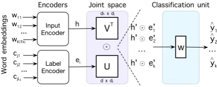
We propose a new output layer parametrization for neural text classification which is composed of a generalized input-label embedding that captures the structure of the labels, the structure of the encoded texts and the interactions between the two, followed by a classification unit which is independent of the label set size. The resulting model has the following properties: (i) it is able to capture complex output structure, (ii) it has a flexible parametrization that allows its capacity to be controlled, and (iii) it is trained with a classification surrogate loss such as cross-entropy. The model is depicted in Figure 1. In this section, we describe the model in detail, showing how it can be trained efficiently for arbitrarily large label sets and how it is related to previous models.

3.1 A Generalized Input-Label Embedding

Letgin(h)andgout(ej) be two nonlinear

projec-tions of the encoded input, namely, the document h, and any encoded label ej, where ej is thejth

h' e2

U

V h' e1 ∧

Classification unit

w

y1 ∧ y2

…

Joint space

h' ek yk ∧

…

Label Encoder

cj1

cj2

cjLj ...

ei Input Encoder

w11

w12

wKiTKi

... h

Encoders

dh x dj

d x dj

W

or

d e

m

be

dd

in

gs

' '

'

T

Figure 1: Each encoded text and label are projected to a joint input-label multiplicative space, the output of which is processed by a classification unit with label-set-size independent parametrization.

row vector from the label embedding matrix E, which have the following form:

e0_j =gout(ej) =σ(ejU +bu) (7)

h0=gin(h) =σ(V h+bv) (8)

whereσ(·)is a nonlinear activation function such as ReLU or Tanh, the matrixU ∈IRd×dj_{and bias} bu ∈ IRdj are the linear projection of the labels,

and the matrixV ∈IRdj×dh _{and biasb}

v ∈IRdjare

the linear projection of the encoded input. Note that the projections for h0 and e0_j could be high-rank or low-rank depending on their initial dimensions and the target joint space dimension. Also letE0 _∈IR|Y|×dj_{be the matrix resulting from} projecting all the outputsejto the joint space, that

is,gout(E).

The conditional output probability distribution can now be rewritten as:

p(y|x)∝exp E0h0

∝exp gout(E)gin(h)

∝exp σ(EU +bu)

| {z }

Label Structure

σ(V h+bv)

| {z }

Input Structure

(9)

Crucially, this function has no label-set-size dependent parameters, unlike W andb in Equa-tion (3). In principle, this parametrizaEqua-tion can be used for both multi-class and multi-label problems by defining the exponential in terms of a softmax and sigmoid functions, respectively. However, in this paper we will focus on the latter.

3.2 Classification Unit

We require that our classification unit parameters depend only on the joint input-label space above. To represent the compatibility between any en-coded input text hi and any encoded label ej

based on multiplicative interactions in the joint space:

g_joint(ij) =gin(hi)gout(ej) (10)

whereis component-wise multiplication. The probability for hi to belong to one of the

k known labels is modeled by a linear unit that maps any point in the joint space into a score which indicates the validity of the combination:

p(_valij) =g_joint(ij) w+b (11)

where w ∈IRdj _{andbare a scalar variables. We} compute the output of this linear unit for each known label which we would like to predict for a given documenti, namely:

P_val(i) =

        

p(_vali1)

p(_vali2)

. . .

p(_valik)

         =         

g_joint(i1) w+b

g_joint(i2) w+b

. . .

g_joint(ik) w+b

         (12)

For each row, the higher the value the more likely the label is to be assigned to the document. To obtain valid probability estimates and be able to train with binary cross-entropy loss for multi-label classification, we apply a sigmoid function as follows:

ˆ

yi= ˆp(yi|xi) =

1

1 +e−Pval(i)

(13)

Summary. By adding the above changes to

the general form of Equation (9) the conditional probability p(yi|xi) is now proportional to the

following quantity:

exp σ(EU+bu)(σ(V h+bv)w) +b

(14)

Note that the number of parameters in this equation is independent of the size of the label set, given thatU,V,w, andbdepend only ondj, andkcan

vary arbitrarily. This allows the model to scale up to large label sets and generalize to unseen labels. Lastly, the proposed output layer addresses all the limitations of the previous models, as follows: (i) it is able to capture complex structure in the joint input–output space, (ii) it provides a means to easily control its capacity dj, and (iii) it is

trainable with cross-entropy loss.

3.3 Training Objectives

The training objective for the multi-label classifi-cation task is based on binary cross-entropy loss. Assuming θ contains all the parameters of the model, the training loss is computed as follows:

L(θ) =− 1 N k N X i=1 k X j=1

H(yij,yˆij) (15)

whereHis the binary cross-entropy between the gold labelyij and predicted labelyˆij for a

docu-mentiand a candidate labelj.

We handle multiple languages according to Firat et al. (2016) and Pappas and Popescu-Belis (2017). Assuming that Θ = {θ1, θ2, ..., θM} are

all the parameters required for each of the M languages, we use a joint multilingual objective based on the sum of cross-entropy losses:

L(Θ) =−1 Z Ne X i M X l k X j=1

H(y_ij(l),yˆ(_ijl)) (16)

where Z = NeM k with Ne being the number

of examples per epoch. At each iteration, a document-label pair for each language is sampled. In addition, multilingual models share a certain subset of the encoder parameters during train-ing while the output layer parameters are kept language-specific, as described by Pappas and Popescu-Belis (2017). In this paper, we share most of the output layer parameters, namely, the ones from the input-label space (U, V,bv,bu), and

we keep only the classification unit parameters (w, b) language-specific.

3.4 Scaling Up to Large Label Sets

For a very large number dj of joint-space

di-mensions in our parametrization, the computa-tional complexity increases prohibitively because our projection requires a large matrix multiplica-tion betweenU andE, which depends on|Y|. In such cases, we resort to sampling-based training by adopting the commonly used negative sampling method proposed by Mikolov et al. (2013). Let xi ∈ IRd andyik ∈ {0,1} be an input-label pair

and yˆik the output probabilities from our model

loss L(θ) in Equation (15) can be re-written as follows:

=−1 Z

N X

i=1

k X

j=1

h

yijlog ˆyij + ¯yijlog (1−yˆij) i

=−1 Z

N X

i=1

h k_ip X

j=1

log ˆyij + kn

i

X

j=1

log (1−yˆij) i

(17)

where Z = N k and y¯ij is (1−yij). To reduce

the computational cost needed to evaluate yˆij

for all the negative label set k_in, we sample k∗ labels from the negative label set with probability p= _|k1n

i| to create the setk

n

i. This enables training

on arbitrarily large label sets without increasing the computation required. By controlling the number of samples we can drastically speed up the training time, as we demonstrate empirically in Section 4.2.2. Exploring more informative sampling methods (e.g., importance sampling) would be an interesting direction of future work.

3.5 Relation to Previous Parametrizations

The proposed embedding form can be seen as a generalization over the input-label embeddings with a bilinear form, because its degenerate form is equivalent to the bilinear form of Equation (5). In particular, this can be simply derived if we set one of the two nonlinear projection functions in the second line of Equation (9) to be the identity function (e.g.,gout(·) =I), set all biases to zero,

and make the σ(.) activation function linear, as follows:

σ(EU +bu)σ(V h+bv) = (EI) (V h)

=EV h (18)

where V by consequence has the same number of dimensions as W ∈ IRd×dh _{from the bilinear} input-label embedding model of Equation (5).

4 Experiments

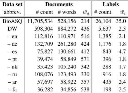
The evaluation is performed on large-scale biomedical semantic indexing using the BioASQ data set, obtained by Nam et al. (2016), and on multilingual news classification using the DW corpus, which consists of eight language data sets obtained by Pappas and Popescu-Belis (2017). The statistics of these data sets are listed in Table 1.

Data set Documents Labels

abbrev. # count # words w¯d # count w¯l

BioASQ 11,705,534 528,156 214 26,104 35.0 DW 598,304 884,272 436 5,637 2.3 – en 112,816 110,971 516 1,385 2.1 – de 132,709 261,280 424 1,176 1.8 – es 75,827 130,661 412 843 4.7 – pt 39,474 58,849 571 396 1.8 – uk 35,423 105,240 342 288 1.7 – ru 108,076 123,493 330 916 1.8 – ar 57,697 58,922 357 435 2.4 – fa 36,282 34,856 538 198 2.5

Table 1: Data set statistics. #count is the number of documents, #words are the number of unique words in the vocabularyV,w¯d andw¯lare the average number

of words per document and label, respectively.

4.1 Biomedical Text Classification

We evaluate on biomedical text classification to demonstrate that our generalized input-label model scales to very large label sets and performs better than previous joint input-label models on both seen and unseen label prediction scenarios.

4.1.1 Settings

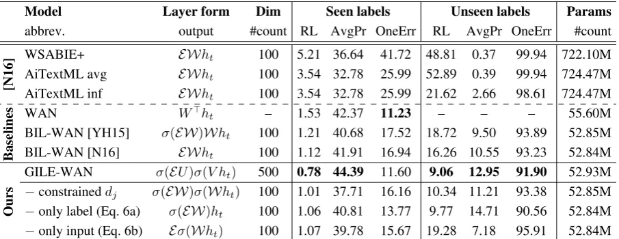
We follow the exact evaluation protocol, data, and settings of Nam et al. (2016), as described below. We use the BioASQ Task 3a data set, which is a collection of scientific publications in biomedical research. The data set contains about 12M documents labeled with around 11 labels out of 27,455, which are defined according to the Medical Subject Headings (MESH) hierarchy. The data were minimally pre-processed with tokenization, number replacements (NUM), rare word replacements (UNK), and split with the provided script by year so that the training set includes all documents until 2004 and the ones from 2005 to 2015 were kept for the test set; this corresponded to 6,692,815 documents for training and 4,912,719 for testing. For validation, a set of 100,000 documents were randomly sampled from the training set. We report the same ranking-based evaluation metrics as Nam et al. (2016), namely, rank loss (RL), average precision (AvgPr), and one-error loss (OneErr).

Model Layer form Dim Seen labels Unseen labels Params

abbrev. output #count RL AvgPr OneErr RL AvgPr OneErr #count

[N16]

WSABIE+ EWht 100 5.21 36.64 41.72 48.81 0.37 99.94 722.10M

AiTextML avg EWht 100 3.54 32.78 25.99 52.89 0.39 99.94 724.47M

AiTextML inf EWht 100 3.54 32.78 25.99 21.62 2.66 98.61 724.47M

Baselines

WAN W>ht – 1.53 42.37 11.23 – – – 55.60M

BIL-WAN [YH15] σ(EW)Wht 100 1.21 40.68 17.52 18.72 9.50 93.89 52.85M

BIL-WAN [N16] EWht 100 1.12 41.91 16.94 16.26 10.55 93.23 52.84M

Ours

GILE-WAN σ(EU)σ(V ht) 500 0.78 44.39 11.60 9.06 12.95 91.90 52.93M

−constraineddj σ(EW)σ(Wht) 100 1.01 37.71 16.16 10.34 11.21 93.38 52.85M

−only label (Eq. 6a) σ(EW)ht 100 1.06 40.81 13.77 9.77 14.71 90.56 52.84M

−only input (Eq. 6b) Eσ(Wht) 100 1.07 39.78 15.67 19.28 7.18 95.91 52.84M

Table 2: Biomedical semantic indexing results computed over labels seen and unseen during training, i.e., the full-resource versus zero-resource settings. Best scores among the competing models are marked inbold.

maximum number of 300 words per document and 50 words per label, ReLU activation, 0.3% negative label sampling, and optimization with ADAM until convergence. The word embeddings were learned end-to-end on the task.4

The baselines are the joint input-label models from Nam et al. (2016), noted as [N16], namely:

• WSABIE+: This model is an extension of the original WSABIE model by Weston et al. (2011), which, instead of learning a ranking model with fixed document features, jointly learns features for documents and words, and is trained with the WARP ranking loss.

• AiTextML: This model is the one proposed by Nam et al. (2016) with the purpose of learning joint representations of documents, labels, and words, along with a joint input-label space that is trained with the WARP ranking loss.

The scores of the WSABIE+ and AiTextML baselines in Table 2 are the ones reported by Nam et al. (2016). In addition, we report scores of a word-level attention neural network (WAN) with DENSE encoder and attention followed by a sigmoid output layer, trained with binary cross-entropy loss.5Our model replaces WAN’s output

4_{Here, the word embeddings are included in the parameter}

statistics because they are variables of the network.

5_{In our preliminary experiments, we also trained the}

neural model with a hinge loss as WSABIE+ and AiTextML, but it performed similarly to them and much worse than WAN, so we did not further experiment with it.

layer with a generalized input-label embedding layer and its variations, noted GILE-WAN. For comparison, we also compare to bilinear input-label embedding versions of WAN for the model by Yazdani and Henderson (2015), noted as BIL-WAN [YH16], and the one by Nam et al. (2016), noted as BIL-WAN [N16]. Note that the AiTextML parameter space is huge and makes learning difficult for our models (linear with respect to labels and documents). Instead, we make sure that our models have far fewer pa-rameters than the baselines (Table 2).

4.1.2 Results

The results on biomedical semantic indexing on seen and unseen labels are shown in Table 2. We observe that the neural baseline, WAN, out-performs WSABIE+ and AiTextML on the seen labels, by +5.73 and +9.59 points in terms of AvgPr, respectively. The differences are even more pronounced when considering the ranking loss and one error metrics. This result is com-patible with previous findings that existing joint input-label models are not able to outperform strong supervised baselines on seen labels. How-ever, WAN is not able to generalize at all to unseen labels, hence the WSABIE+ and AiTextML have a clear advantage in the zero-resource setting.

on unseen labels. GILE-WAN outperforms WSABIE+ and AiTextML variants6 _{by a large} margin in both cases—for example, by +7.75, +11.61 points on seen labels and by +12.58, +10.29 points in terms of average precision on unseen labels, respectively. Interestingly, our GILE-WAN model also outperforms the two previous bilinear input-label embedding formulations of Yazdani and Henderson (2015) and Nam et al. (2016), namely, BIL-WAN [YH15] and BIL-WAN [N16], by +3.71, +2.48 points on seen labels and +3.45 and +2.39 points on unseen labels, respectively, even when they are trained with the same encoders and loss as ours. These models are not able to outperform the WAN baseline when evaluated on the seen labels, that is they have

−1.68 and−0.46 points lower average precision than WAN, but they outperform WSABIE+ and AiTextML on both seen and unseen labels. Overall, the results show a clear advantage of our generalized input-label embedding model against previous models on both seen and unseen labels.

4.1.3 Ablation Analysis

To evaluate the effectiveness of individual com-ponents of our model, we performed an ablation study (last three rows in Table 2). Note that when we use only the label or only the input embedding in our generalized input-label formulation, the dimensionality of the joint space is constrained to be the dimensionality of the encoded labels and inputs respectively (i.e., dj=100 in our

experiments).

All three variants of our model outperform previous embedding formulations of Nam et al. (2016) and Yazdani and Henderson (2015) in all metrics except for AvgPr on seen labels, where they score slightly lower. The decrease in AvgPrec for our model variants with dj=100 compared

with the neural baselines could be attributed to the difficulty in learning the parameters of a highly nonlinear space with only a few hid-den dimensions. Indeed, when we increase the number of dimensions (dj=500), our full model

outperforms them by a large margin. Recall that this increase in capacity is only possible with our full model definition in Equation (9) and none of the other variants allow us to do this without

6_{Namely,avg when using the average of word vectors}

andinfwhen using inferred label vectors to make predictions.

interfering with the original dimensionality of the encoded labels (E) and input (ht). In addition, our

model variants withdj=100exhibit consistently

higher scores than baselines in terms of most metrics on both seen and unseen labels, which suggests that they are able to capture more complex relationships across labels and between encoded inputs and labels.

Overall, the best performance among our model variants is achieved when using only the label embedding and, hence, it is the most significant component of our model. Surprisingly, our model with only the label embedding achieves higher performance than our full model on unseen labels but it is far behind our full model when we consider performance on both seen and unseen labels. When we constrain our full model to have the same dimensionality with the other variants (i.e., dj=100), it outperforms the one that uses

only the input embedding in most metrics and it is outperformed by the one that uses only the label embedding.

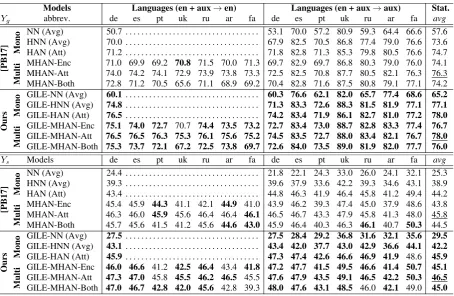
4.2 Multilingual News Text Classification

We evaluate on multilingual news text clas-sification to demonstrate that our output layer based on the generalized input-label embedding outperforms previous models with a typical output layer in a wide variety of settings, even for labels that have been seen during training.

4.2.1 Settings

We follow the exact evaluation protocol, data, and settings of Pappas and Popescu-Belis (2017), as described below. The data set is split per language into 80% for training, 10% for validation, and 10% for testing. We evaluate on both types of labels (general Yg, and specific Ys) in a

full-resource scenario, and we evaluate only on the general labels (Yg) in a low-resource scenario.

Accuracy is measured with the micro-averaged F1 percentage scores.

The word embeddings for this task are the aligned pre-trained 40-dimensional multi-CCA multilingual word embeddings by Ammar et al. (2016) and are kept fixed during training.7 _The sentences are already truncated at a length of 30 words and the documents at a length of 30 sentences. The hyper-parameters were selected

7_{The word embeddings are not included in the parameters}

Models Languages (en + aux→en) Languages (en + aux→aux) Stat.

Yg abbrev. de es pt uk ru ar fa de es pt uk ru ar fa avg

[PB17]

Mono

NN (Avg) 50.7 . . . 53.1 70.0 57.2 80.9 59.3 64.4 66.6 57.6 HNN (Avg) 70.0 . . . 67.9 82.5 70.5 86.8 77.4 79.0 76.6 73.6 HAN (Att) 71.2 . . . 71.8 82.8 71.3 85.3 79.8 80.5 76.6 74.7

Multi

MHAN-Enc 71.0 69.9 69.2 70.8 71.5 70.0 71.3 69.7 82.9 69.7 86.8 80.3 79.0 76.0 74.1 MHAN-Att 74.0 74.2 74.1 72.9 73.9 73.8 73.3 72.5 82.5 70.8 87.7 80.5 82.1 76.3 76.3 MHAN-Both 72.8 71.2 70.5 65.6 71.1 68.9 69.2 70.4 82.8 71.6 87.5 80.8 79.1 77.1 74.2

Ours

Mono

GILE-NN (Avg) 60.1. . . 60.3 76.6 62.1 82.0 65.7 77.4 68.6 65.2 GILE-HNN (Avg) 74.8. . . 71.3 83.3 72.6 88.3 81.5 81.9 77.1 77.1 GILE-HAN (Att) 76.5. . . 74.2 83.4 71.9 86.1 82.7 81.0 77.2 78.0

Multi

GILE-MHAN-Enc 75.1 74.0 72.7 70.7 74.4 73.5 73.2 72.7 83.4 73.0 88.7 82.8 83.3 77.4 76.7 GILE-MHAN-Att 76.5 76.5 76.3 75.3 76.1 75.6 75.2 74.5 83.5 72.7 88.0 83.4 82.1 76.7 78.0 GILE-MHAN-Both 75.3 73.7 72.1 67.2 72.5 73.8 69.7 72.6 84.0 73.5 89.0 81.9 82.0 77.7 76.0

Ys Models de es pt uk ru ar fa de es pt uk ru ar fa avg

[PB17]

Mono

NN (Avg) 24.4 . . . 21.8 22.1 24.3 33.0 26.0 24.1 32.1 25.3 HNN (Avg) 39.3 . . . 39.6 37.9 33.6 42.2 39.3 34.6 43.1 38.9 HAN (Att) 43.4 . . . 44.8 46.3 41.9 46.4 45.8 41.2 49.4 44.2

Multi

MHAN-Enc 45.4 45.9 44.3 41.1 42.1 44.9 41.0 43.9 46.2 39.3 47.4 45.0 37.9 48.6 43.8 MHAN-Att 46.3 46.0 45.9 45.6 46.4 46.4 46.1 46.5 46.7 43.3 47.9 45.8 41.3 48.0 45.8 MHAN-Both 45.7 45.6 41.5 41.2 45.6 44.6 43.0 45.9 46.4 40.3 46.3 46.1 40.7 50.3 44.5

Ours

Mono

GILE-NN (Avg) 27.5. . . 27.5 28.4 29.2 36.8 31.6 32.1 35.6 29.5 GILE-HNN (Avg) 43.1. . . 43.4 42.0 37.7 43.0 42.9 36.6 44.1 42.2 GILE-HAN (Att) 45.9. . . 47.3 47.4 42.6 46.6 46.9 41.9 48.6 45.9

Multi

GILE-MHAN-Enc 46.0 46.6 41.2 42.5 46.4 43.4 41.8 47.2 47.7 41.5 49.5 46.6 41.4 50.7 45.1 GILE-MHAN-Att 47.3 47.0 45.8 45.5 46.2 46.5 45.5 47.6 47.9 43.5 49.1 46.5 42.2 50.3 46.5 GILE-MHAN-Both 47.0 46.7 42.8 42.0 45.6 42.8 39.3 48.0 47.6 43.1 48.5 46.0 42.1 49.0 45.0

Table 3: Full-resource classification results on general (upper half) and specific (lower half) labels using monolingual and bilingual models with DENSEencoders on English as target (left) and the auxiliary language as

target (right). The average bilingual F1-score (%) is notedavgand the top ones per block are underlined. The monolingual scores on the left come from a single model, hence a single score is repeated multiple times; the repetition is marked with consecutive dots.

on validation data as follows: 100-dimensional encoder and attention, ReLU activation, batch size 16, epoch size 25k, no negative sampling (all labels are used), and optimization with ADAM until convergence. To ensure equal capacity to baselines, we use approximately the same number of parametersntotwith the baseline classification

layers, by setting:

dj '

dh∗ |k(i)|

dh+d

, i= 1, . . . , M (19)

in the monolingual case, and similarly, dj '

(dh ∗ PMi=1|k(i)|)/(dh+d) in the multilingual

case, where k(i) is the number of labels in lan-guagei.

The hierarchical models have Dense encoders in all scenarios (Tables 3, 6, and 7), except from the varying encoder experiment (Table 4). For the low-resource scenario, the levels of data availability are: tiny from 0.1% to 0.5%, small

from 1% to 5% and medium from 10% to 50% of the original training set. For each level, the average F1 across discrete increments of 0.1, 1

and 10 are reported respectively. The decision thresholds, which were tuned on validation data by Pappas and Popescu-Belis (2017), are set as follows: for the full-resource scenario it is set to 0.4 for |Ys| < 400 and 0.2 for |Ys| ≥ 400, and

for the low-resource scenario it is set to 0.3 for all sets.

The baselines are all the monolingual and multilingual neural networks from Pappas and Popescu-Belis (2017),8noted as [PB17], namely:

• NN: A neural network that feeds the av-erage vector of the input words directly to a classification layer, as the one used by Klementiev et al. (2012).

• HNN: A hierarchical network with encoders and average pooling at every level, followed by a classification layer, as the one used by Tang et al. (2015).

8_{For reference, in Table 4 we also compare to a logistic}

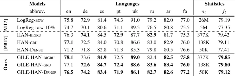
Models Languages Statistics

abbrev. en de es pt uk ru ar fa nl fl

[M17]

LogReg-BOW 75.8 72.9 81.4 74.3 91.0 79.2 82.0 77.0 26M 79.19

LogReg-BOW-10% 74.7 70.1 80.6 71.1 89.5 76.5 80.8 75.5 5M 77.35

[PB17]

HAN-BIGRU 76.3 74.1 84.5 72.9 87.7 82.9 81.7 75.3 377K 79.42

HAN-GRU 77.1 72.5 84.0 70.8 86.6 83.0 82.9 76.0 138K 79.11

HAN-DENSE 71.2 71.8 82.8 71.3 85.3 79.8 80.5 76.6 50K 77.41

Ours

GILE-HAN-BIGRU 78.1 73.6 84.9 72.5 89.0 82.4 82.5 75.8 377K 79.85

GILE-HAN-GRU 77.1 72.6 84.7 72.4 88.6 83.6 83.4 76.0 138K 79.80

GILE-HAN-DENSE 76.5 74.2 83.4 71.9 86.1 82.7 82.6 77.2 50K 79.12

Table 4: Full-resource classification results on general (Yg) topic labels with DENSEandGRUencoders. Reported

are also the average number of parameters per language (nl) and the averageF1per language (fl).

• HAN: A hierarchical network with encoders and attention, followed by a classification layer, as the one used by Yang et al. (2016).

• MHAN: Three multilingual hierarchical net-works with shared encoders, noted MHAN-Enc, shared attention, noted MHAN-Att, and shared attention and encoders, noted MHAN-Both, as the ones used by Pappas and Popescu-Belis (2017).

To ensure a controlled comparison to the above baselines, for each model we evaluate a version where their output layer is replaced by our generalized input-label embedding output layer using the same number of parameters; these have the abbreviation ‘‘GILE’’ prepended in their name (e.g., GILE-HAN). The scores of HAN and MHAN models in Tables 3, 6, and 7 are the ones reported by Pappas and Popescu-Belis (2017), while for Table 4 we train them ourselves using their code. Lastly, the best score for each pairwise comparison between a joint input-label model and its counterpart is marked inbold.

4.2.2 Results

Table 3 displays the results of full-resource docu-ment classification using DENSEencoders for both general and specific labels. On the left, we display the performance of models on the English sub-corpus when English and an auxiliary language are used for training, and on the right, the performance on the auxiliary language sub-corpus when that language and English are used for training.

The results show that in 98% of comparisons on general labels (top half of Table 3) the joint input-label models improve consistently over the

corresponding models using a typical sigmoid classification layer. This finding validates our main hypothesis that the joint input-label models successfully exploit the semantics of the labels, which provide useful cues for classification, as opposed to models which are agnostic to label semantics. The results for specific labels (bottom half of Table 3) demonstrate the same trend, with the joint input-label models performing better in 87% of comparisons.

HAN Languages

Ygoutput layer en de es pt uk ru ar fa

Linear [PB17] 71.2 71.8 82.8 71.3 85.3 79.8 80.5 76.6

BIL [YH15] 71.7 70.5 82.0 71.1 86.6 80.6 80.4 76.0

BIL [N16] 69.8 69.1 80.9 67.4 87.5 79.9 78.4 75.1

GILE (Ours) 76.5 74.2 83.4 71.9 86.1 82.7 82.6 77.2

- constraineddj 73.6 73.1 83.3 71.0 87.1 81.6 80.4 76.4

- only label 71.4 69.6 82.1 70.3 86.2 80.6 81.1 76.2

- only input 55.1 54.2 80.6 66.5 85.6 60.8 78.9 74.0

Ysoutput layer en de es pt uk ru ar fa

Linear[PB17] 43.4 44.8 46.3 41.9 46.4 45.8 41.2 49.4

BIL [YH15] 40.7 37.8 38.1 33.5 44.6 38.1 39.1 42.6

BIL [N16] 34.4 30.2 34.4 33.6 31.4 22.8 35.6 38.9

GILE (Ours) 45.9 47.3 47.4 42.6 46.6 46.9 41.9 48.6

- constraineddj 38.5 38.0 36.8 35.1 42.1 36.1 36.7 48.7

- only label 38.4 41.5 42.9 38.3 44.0 39.3 37.2 43.4

- only input 12.1 10.8 8.8 20.5 11.8 7.8 12.0 24.6

Table 5: Direct comparison with previous bilinear input-label models, namely, BIL [YH15] and BIL [N16], and with our ablated model variants using the best monolingual configuration (HAN) from Table 3 on both general (upper half) and specific (lower half) labels. Best scores among the competing models are marked inbold.

The best bilingual performance on average is that of the GILE-MHAN-Att model, for both general and specific labels. This improvement can be attributed to the effective sharing between label semantics across languages through the joint multilingual input-label output layer. Effectively, this model has the same multilingual sharing scheme with the best model reported by Pappas and Popescu-Belis (2017), MHAN-Att, namely, sharing attention at each level of the hierarchy, which agrees well with their main finding.

Interestingly, the improvement holds when using different types of hierarchical encoders, namely, DENSE GRU, and biGRU, as shown in Table 4, which demonstrate the generality of the approach. In addition, our best models outperform logistic regression trained either on top-10% most frequent words or on the full vocabulary, even though our models utilize many fewer parameters, that is, 377K/138K vs. 26M/5M. Increasing the capacity of our models should lead to even further improvements.

Multilingual learning. So far, we have shown that the proposed joint input-label models out-perform typical neural models when training with one and two languages. Does the improvement remain when increasing the number of languages even more? To answer the question we report in Table 6 the average F1-score per language for the best baselines from the previous experiment (HAN and MHAN-Att) with the proposed joint

Models General labels Specific labels

abbrev. # lang. nl fl nl fl

[PB17]

HAN 1 50K 77.41 90K 44.90

MHAN 2 40K 78.30 80K 45.72 MHAN 8 32K 77.91 72K 45.82

Ours

GILE-HAN 1 50K 79.12 90K 45.90

GILE-MHAN 2 40K 79.68 80K 46.49

GILE-MHAN 8 32K 79.48 72K 46.32

Table 6: Multilingual learning results. The columns are the average number of parameters per language (nl), averageF1per language (fl).

input-label versions of them (GILE-HAN and GILE-MHAN-Att) when increasing the number of languages (1, 2, and 8) that are used for train-ing. Overall, we observe that the joint input-label models outperform all the baselines independently of the number of languages involved in the train-ing, while having the same number of parameters. We also replicate the previous result that a second language helps but beyond that there is no improvement.

Low-resource transfer. We investigate here

Levels [PB17] Ours

range HAN MHAN GILE-MHAN

en

→

de 0.1-0.5% 29.9 39.4 42.9

1-5% 51.3 52.6 51.6

10-50% 63.5 63.8 65.9

en

→

es 0.1-0.5% 39.5 41.5 39.0

1-5% 45.6 50.1 50.9

10-50% 74.2 75.2 76.4

en

→

pt 0.1-0.5% 30.9 33.8 39.6

1-5% 44.6 47.3 48.9

10-50% 60.9 62.1 62.3

en

→

uk 0.1-0.5% 60.4 60.9 61.1

1-5% 68.2 69.0 69.4

10-50% 76.4 76.7 76.5

en

→

ru 0.1-0.5% 27.6 29.1 27.9

1-5% 39.3 40.2 40.2

10-50% 69.2 69.4 70.4

en

→

ar 0.1-0.5% 35.4 36.6 46.1

1-5% 45.6 46.6 49.5

10-50% 48.9 47.8 61.8

en

→

fa 0.1-0.5% 36.0 41.3 42.5

1-5% 55.0 55.5 55.4

10-50% 69.2 70.0 69.7

Table 7: Low-resource classification results with various sizes of training data using the general labels.

(Yang et al., 2016) and MHAN (Pappas and Popescu-Belis, 2017), for low-resource classifi-cation in the majority of the cases.

The shared input-label space appears to be helpful especially when transferring from English to German, Portuguese, and Arabic languages. GILE-MHAN is significantly behind MHAN on transferring knowledge from English to Spanish and to Russian in the 0.1% to 0.5% resource setting, but in the rest of the cases they have very similar scores.

Label sampling. To speed up computation it is possible to train our model by sampling labels, instead of training over the whole label set. How much speed-up can we achieve from this label sampling approach and still retain good levels of performance? In Figure 2, we attempt to answer this question by reporting the performance of our GILE-HNN model when varying the amount of labels (%) that it uses for training over English general and specific labels of the DW data set. In both cases, the performance of GILE-HNN tends to increase as the percentage of labels sampled increases, but it levels off for the higher percentages.

Figure 2: Varying sampling percentage for general and specific English labels.(Top)GILE-HNN is compared against HNN in terms of F1 (%).(Bottom)The runtime speed-up over GILE-HNN trained on the full label set.

For general labels, top performance is reached with a 40% to 50% sampling rate, which translates to a 22% to 18% speed-up, whereas for the specific labels, it is reached with a 60% to 70% sampling rate, which translates to a 40% to 36% speed-up. The speed-up is correlated to the size of the label set, since there are many fewer general labels than specific labels, namely, 327 vs. 1,058 here. Hence, we expect even higher speedups for bigger label sets. Interestingly, GILE-HNN with label sampling reaches the performance of the baseline with a 25% and 60% sample for general and specific labels respectively. This translates to a speed-up of 30% and 50%, respectively, compared with a GILE-HNN trained over all labels. Overall, these results show that our model is effective and that it can also scale to large label sets. The label sampling should also be useful in tasks where the computation resources may be limited or budgeted.

5 Related Work

5.1 Neural text Classification

information, which outperformed simpler CNNs. Lin et al. (2015) and Tang et al. (2015) pro-posed hierarchical recurrent neural networks and showed that they were superior to CNN-based models. Yang et al. (2016) demonstrated that a hierarchical attention network with bi-directional gated encoders outperforms previous alternatives. Pappas and Popescu-Belis (2017) adapted such networks to learn hierarchical document structures with shared components across different languages.

The issue of scaling to large label sets has been addressed previously by output layer approx-imations (Morin and Bengio, 2005) and with the use of sub-word units or character-level modeling (Sennrich et al., 2016; Lee et al., 2017) which is mainly applicable to structured prediction problems. Despite the numerous stud-ies, most of the existing neural text classification models ignore label descriptions and semantics. Moreover, they are based on typical output layer parametrizations that are dependent on the label set size, and thus are not able to scale well to large label sets nor to generalize to unseen labels. Our output layer parametrization addresses these limitations and could potentially improve such models.

5.2 Output Representation Learning

There exist studies that aim to learn output rep-resentations directly from data without any seman-tic grounding to word embeddings (Srikumar and Manning, 2014; Yeh et al., 2018; Augenstein et al., 2018). Such methods have a label-set-size dependent parametrization, which makes them data hungry, less scalable on large label sets, and incapable of generalizing to unseen classes. Wang et al. (2018) addressed the lack of semantic grounding to word embeddings by proposing an efficient method based on label-attentive text rep-resentations which are helpful for text clas-sification. However, in contrast to our study, their parametrization is still label-set-size dependent and thus their model is not able to scale well to large label sets nor to generalize to unseen labels.

5.3 Zero-shot Text Classification

Several studies have focused on learning joint input-label representations grounded to word semantics for unseen label prediction for images (Weston et al., 2011; Socher et al., 2013; Norouzi et al., 2014; Zhang et al., 2016; Fu et al., 2018),

called zero-shot classification. However, there are fewer such studies for text classification. Dauphin et al. (2014) predicted semantic utterances of text by mapping them in the same semantic space with the class labels using an unsupervised learn-ing objective. Yazdani and Henderson (2015) pro-posed a zero-shot spoken language understanding model based on a bilinear input-label model able to generalize to previously unseen labels. Nam et al. (2016) proposed a bilinear joint document-label embedding that learns shared word representations between documents and labels. More recently, Shu et al. (2017) proposed an approach for open-world classification that aims to identify novel docu-ments during testing but it is not able to generalize to unseen classes. Perhaps the model most similar to ours is from the recent study by Pappas et al. (2018) on neural machine translation, with the difference that they have single-word label des-criptions and they use a label-set-dependent bias in a softmax linear prediction unit, which is designed for structured prediction. Hence, their model can neither handle unseen labels nor multi-label classification, as we do here.

Compared with previous joint input-label models, the proposed model has a more general and flexible parametrization, which allows the output layer capacity to be controlled. Moreover, it is not restricted to linear mappings, which have limited expressivity, but uses nonlinear mappings, similar to energy-based learning networks (LeCun et al., 2006; Belanger and McCallum, 2016). The link to the latter can be made if we regard P_val(ij) in Equation (11) as an energy function for thei-th document and the j-th label, the calculation of which uses a simple multiplicative transformation (Equation (10)). Lastly, the proposed model performs well on both seen and unseen label sets by leveraging the binary cross-entropy loss, which is the standard loss for classification problems, instead of a ranking loss.

6 Conclusion

with previous joint input-label models, it performs significantly better on unseen labels without compromising performance on the seen labels. These improvements can be attributed to the the ability of our model to capture complex input-label relationships, to its controllable capacity, and to its training objective, which is based on cross-entropy loss.

As future work, the label representation could be learned by a more sophisticated encoder, and the label sampling could benefit from importance sampling to avoid revisiting uninformative labels. Another interesting direction would be to find a more scalable way of increasing the output layer capacity—for instance, using a deep rather than a wide classification network. Moreover, adapting the proposed model to structured prediction, for instance by using a softmax classification unit instead of a sigmoid one, would benefit tasks such as neural machine translation, language modeling, and summarization in isolation but also when trained jointly with multi-task learning.

Acknowledgments

We are grateful for the support from the European Union through its Horizon 2020 program in the SUMMA project n. 688139, see http://www. summa-project.eu. We would also like to thank our action editor, Eneko Agirre, and the anonymous reviewers for their invaluable suggestions and feedback.

References

Waleed Ammar, George Mulcaire, Yulia Tsvetkov, Guillaume Lample, Chris Dyer, and Noah A. Smith. 2016. Massively multilingual word em-beddings.CoRR, abs/1602.01925.v2.

Isabelle Augenstein, Sebastian Ruder, and Anders Søgaard. 2018. Multi-task learning of pairwise sequence classification tasks over disparate label spaces. In Proceedings of the 2018 Conference of the North American Chapter of the Association for Computational Linguistics: Human Language Technologies, Volume 1 (Long Papers), pages 1896–1906. New Orleans, Louisiana.

David Belanger and Andrew McCallum. 2016. Structured prediction energy networks. In Pro-ceedings of The 33rd International Conference on

Machine Learning, volume 48 of Proceedings of Machine Learning Research, pages 983–992, New York, New York, USA. PMLR.

Jianshu Chen, Ji He, Yelong Shen, Lin Xiao, Xiaodong He, Jianfeng Gao, Xinying Song, and Li Deng. 2015. End-to-end learning of LDA by mirror-descent back propagation over a deep architecture. InAdvances in Neural Information Processing Systems 28, pages 1765–1773. Montreal, Canada.

Kyunghyun Cho, Bart van Merrienboer, Caglar Gulcehre, Dzmitry Bahdanau, Fethi Bougares, Holger Schwenk, and Yoshua Bengio. 2014. Learning phrase representations using RNN encoder–decoder for statistical machine trans-lation. InProceedings of the 2014 Conference on Empirical Methods in Natural Language Processing, pages 1724–1734, Doha, Qatar.

Ronan Collobert, Jason Weston, L´eon Bottou, Michael Karlen, Koray Kavukcuoglu, and Pavel Kuksa. 2011. Natural language processing (almost) from scratch. Journal of Machine Learning Research, 12:2493–2537.

Yann N. Dauphin, G¨okhan T¨ur, Dilek Hakkani-T¨ur, and Larry P. Heck. 2014. Zero-shot learning and clustering for semantic utterance classification. In International Conference on Learning Representations. Banff, Canada.

Orhan Firat, Baskaran Sankaran, Yaser Al-Onaizan, Fatos T. Yarman Vural, and Kyunghyun Cho. 2016. Zero-resource lation with multi-lingual neural machine trans-lation. InProceedings of the 2016 Conference on Empirical Methods in Natural Language Processing, pages 268–277, Austin, USA.

Andrea Frome, Greg S. Corrado, Jon Shlens, Samy Bengio, Jeff Dean, Marc Aurelio Ranzato, and Tomas Mikolov. 2013. DeViSE: A deep visual-semantic embedding model, In C. J. C. Burges, L. Bottou, M. Welling, Z. Ghahramani, and K. Q. Weinberger, editors, Advances in Neural Information Processing Systems 26, pages 2121–2129. Curran Associates, Inc.

recognition: Toward data-efficient understand-ing of visual content. IEEE Signal Processing Magazine, 35(1):112–125.

Rie Johnson and Tong Zhang. 2015. Effective use of word order for text categorization with convolutional neural networks. InProceedings of the 2015 Conference of the North American Chapter of the Association for Computational Linguistics: Human Language Technologies, pages 103–112, Denver, Colorado.

Yoon Kim. 2014. Convolutional neural networks for sentence classification. In Proceedings of the 2014 Conference on Empirical Methods in Natural Language Processing, pages 1746–1751, Doha, Qatar.

Alexandre Klementiev, Ivan Titov, and Binod Bhattarai. 2012. Inducing crosslingual dis-tributed representations of words. In Pro-ceedings of COLING 2012, pages 1459–1474, Mumbai, India.

Ankit Kumar, Ozan Irsoy, Jonathan Su, James Bradbury, Robert English, Brian Pierce, Peter Ondruska, Ishaan Gulrajani, and Richard Socher. 2015. Ask me anything: Dynamic mem-ory networks for natural language processing. InProceedings of The 33rd International Con-ference on Machine Learning, pages 334–343, New York City, USA.

Siwei Lai, Liheng Xu, Kang Liu, and Jun Zhao. 2015. Recurrent convolutional neural networks for text classification. InProceedings of the 29th AAAI Conference on Artificial Intelligence, pages 2267–2273, Austin, USA.

Quoc V. Le and Tomas Mikolov. 2014. Distributed representations of sentences and documents. In

Proceedings of The 31st International Confer-ence on Machine Learning, pages 1188–1196, Beijing, China.

Yann LeCun, Sumit Chopra, Raia Hadsell, Fu Jie Huang, and et al. 2006. A tutorial on energy-based learning. InPredicting Structured Data. MIT Press.

Jason Lee, Kyunghyun Cho, and Thomas Hofmann. 2017. Fully character-level neural machine translation without explicit segmentation. Tran-sactions of the Association for Computational Linguistics, 5:365–378.

Rui Lin, Shujie Liu, Muyun Yang, Mu Li, Ming Zhou, and Sheng Li. 2015. Hierarchical re-current neural network for document model-ing. In Proceedings of the 2015 Conference on Empirical Methods in Natural Language Processing, pages 899–907. Lisbon, Portugal.

Thang Luong, Hieu Pham, and Christopher D. Manning. 2015. Effective approaches to attention-based neural machine translation. In

Proceedings of the 2015 Conference on Empir-ical Methods in Natural Language Processing, pages 1412–1421, Lisbon, Portugal.

Thomas Mensink, Jakob Verbeek, Florent Perronnin, and Gabriela Csurka. 2012. Metric learning for large scale image classification: Generalizing to new classes at near-zero cost. In

Computer Vision – ECCV 2012, pages 488–501, Berlin, Heidelberg. Springer Berlin Heidelberg.

Tomas Mikolov, Ilya Sutskever, Kai Chen, Greg S Corrado, and Jeff Dean. 2013. Distributed representations of words and phrases and their compositionality. In C. J. C. Burges, L. Bottou, M. Welling, Z. Ghahramani, and K. Q. Weinberger, editors, Advances in Neural Information Processing Systems 26, pages 3111–3119. Curran Associates, Inc.

Frederic Morin and Yoshua Bengio. 2005. Hier-archical probabilistic neural network language model. In Proceedings of the Tenth Interna-tional Workshop on Artificial Intelligence and Statistics, pages 246–252.

Khalil Mrini, Nikolaos Pappas, and Andrei Popescu-Belis. 2017. Cross-lingual transfer for news article labeling: Benchmarking statistical and neural models. In Idiap Research Report, Idiap-RR-26-2017.

Jinseok Nam, Eneldo Loza Menc´ıa, and Johannes F¨urnkranz. 2016. All-in text: Learning docu-ment, label, and word representations jointly. In Proceedings of the 13th AAAI Confer-ence on Artificial IntelligConfer-ence, AAAI’16, pages 1948–1954, Phoenix, Arizona.

Conference on Learning Representations, Banff, Canada.

Bo Pang and Lillian Lee. 2005. Seeing stars: Exploiting class relationships for sentiment categorization with respect to rating scales. In Proceedings of the 43rd Annual Meeting on Association for Computational Linguistics, pages 115–124, Ann Arbor, Michigan.

Nikolaos Pappas, Lesly Miculicich, and James Henderson. 2018. Beyond weight tying: Learn-ing joint input-output embeddLearn-ings for neural machine translation. InProceedings of the Third Conference on Machine Translation: Research Papers, pages 73–83, Belgium, Brussels. Association for Computational Linguistics.

Nikolaos Pappas and Andrei Popescu-Belis. 2017. Multilingual hierarchical attention networks for document classification. In Proceedings of the Eighth International Joint Conference on Natural Language Processing (Volume 1: Long Papers), pages 1015–1025.

Alexander M. Rush, Sumit Chopra, and Jason Weston. 2015. A neural attention model for abstractive sentence summarization. In Pro-ceedings of the 2015 Conference on Empirical Methods in Natural Language Processing, pages 379–389. Lisbon, Portugal.

Rico Sennrich, Barry Haddow, and Alexandra Birch. 2016. Neural machine translation of rare words with subword units. In Proceedings of the 54th Annual Meeting of the Association for Computational Linguistics (Volume 1: Long Papers), pages 1715–1725, Berlin, Germany.

Lei Shu, Hu Xu, and Bing Liu. 2017. DOC: Deep open classification of text documents. In Proceedings of the 2017 Conference on Empirical Methods in Natural Language Processing, pages 2911–2916, Copenhagen, Denmark. Association for Computational Linguistics.

Richard Socher, Milind Ganjoo, Christopher D. Manning, and Andrew Y. Ng. 2013. Zero-shot learning through cross-modal transfer. In Proceedings of the 26th International Conference on Neural Information Processing Systems, NIPS’13, pages 935–943, Lake Tahoe, Nevada.

Vivek Srikumar and Christopher D. Manning. 2014. Learning distributed representations for structured output prediction. InProceedings of the 27th International Conference on Neural Information Processing Systems - Volume 2, NIPS’14, pages 3266–3274, Cambridge, MA, USA. MIT Press.

Duyu Tang, Bing Qin, and Ting Liu. 2015. Document modeling with gated recurrent neural network for sentiment classification. In Proceedings of the 2015 Conference on Empirical Methods in Natural Language Pro-cessing, pages 1422–1432, Lisbon, Portugal. Association for Computational Linguistics.

Guoyin Wang, Chunyuan Li, Wenlin Wang, Yizhe Zhang, Dinghan Shen, Xinyuan Zhang, Ricardo Henao, and Lawrence Carin. 2018. Joint embedding of words and labels for text classification. In Proceedings of the 56th Annual Meeting of the Association for Computational Linguistics (Volume 1: Long Papers), pages 2321–2331. Association for Computational Linguistics.

Jason Weston, Samy Bengio, and Nicolas Usunier. 2010. Large scale image annotation: Learning to rank with joint word-image embeddings.Mach. Learn., 81(1):21–35.

Jason Weston, Samy Bengio, and Nicolas Usunier. 2011. WSABIE: Scaling up to large vocabulary image annotation. In Proceedings of the Twenty-Second International Joint Con-ference on Artificial Intelligence (Volume 3), pages 2764–2770, Barcelona, Spain.

Zichao Yang, Diyi Yang, Chris Dyer, Xiaodong He, Alex Smola, and Eduard Hovy. 2016. Hierarchical attention networks for document classification. InProceedings of the 2016 Con-ference of the North American Chapter of the-Association for Computational Linguistics: Human Language Technologies, pages 1480–1489, San Diego, California.

Chih-Kuan Yeh, Wei-Chieh Wu, Wei-Jen Ko, and Yu-Chiang Frank Wang. 2018. Learning deep latent spaces for multi-label classification. In

Proceedings of the 32nd AAAI Conference on Artificial Intelligence, New Orleans, USA.

Xiang Zhang, Junbo Zhao, and Yann LeCun. 2015. Character-level convolutional networks for text

classification. In Advances in Neural Infor-mation Processing Systems 28, pages 649–657, Montreal, Canada.