Replicability Analysis for Natural Language Processing: Testing
Significance with Multiple Datasets
Rotem Dror Gili Baumer
Faculty of Industrial Engineering and Management, Technion, IIT
{rtmdrr@campus|sgbaumer@campus|marinabo|roiri}.technion.ac.il
Marina Bogomolov Roi Reichart
Abstract
With the ever growing amount of textual data from a large variety of languages, domains, and genres, it has become standard to evalu-ate NLP algorithms on multiple datasets in or-der to ensure a consistent performance across heterogeneous setups. However, such multi-ple comparisonspose significant challenges to traditional statistical analysis methods in NLP and can lead to erroneous conclusions. In this paper we propose aReplicability Analy-sisframework for a statistically sound anal-ysis of multiple comparisons between algo-rithms for NLP tasks. We discuss the theo-retical advantages of this framework over the current, statistically unjustified, practice in the NLP literature, and demonstrate its empirical value across four applications: multi-domain dependency parsing, multilingual POS tag-ging, cross-domain sentiment classification and word similarity prediction.1
1 Introduction
The field of Natural Language Processing (NLP) is going through the data revolution. With the persis-tent increase of the heterogeneous web, for the first time in human history, written language from mul-tiple languages, domains, and genres is now abun-dant. Naturally, the expectations from NLP algo-rithms also grow and evaluating a new algorithm on as many languages, domains, and genres as possible is becoming a de-facto standard.
1Our code is at:
https://github.com/rtmdrr/replicability-analysis-NLP .
For example, the phrase structure parsers of Char-niak (2000) and Collins (2003) were mostly evalu-ated on the Wall Street Journal Penn Treebank (Mar-cus et al., 1993), consisting of written, edited En-glish text of economic news. In contrast, modern dependency parsers are expected to excel on the 19 languages of the CoNLL 2006-2007 shared tasks on multilingual dependency parsing (Buchholz and Marsi, 2006; Nilsson et al., 2007), and additional challenges, such as the shared task on parsing mul-tiple English Web domains (Petrov and McDonald, 2012), are continuously proposed.
Despite the growing number of evaluation tasks, the analysis toolbox employed by NLP researchers has remained quite stable. Indeed, in most exper-imental NLP papers, several algorithms are com-pared on a number of datasets where the perfor-mance of each algorithm is reported together with per-dataset statistical significance figures. However, with the growing number of evaluation datasets, it becomes more challenging to draw comprehensive conclusions from such comparisons. This is because although the probability of drawing an erroneous conclusion from a single comparison is small, with multiple comparisons the probability of making one or more false claims may be very high.
The goal of this paper is to provide the NLP com-munity with a statistical analysis framework, which we termReplicability Analysis, which will allow us to draw statistically sound conclusions in evalua-tion setups that involve multiple comparisons. The classical goal of replicability analysis is to examine the consistency of findings across studies in order to address the basic dogma of science, that a
find-471
ing is more convincingly true if it is replicated in at least one more study (Heller et al., 2014; Patil et al., 2016). We adapt this goal to NLP, where we wish to ascertain the superiority of one algorithm over another across multiple datasets, which may come from different languages, domains, and gen-res. Finding that one algorithm outperforms another across domains gives a sense of consistency to the results and positive evidence that the better perfor-mance is not specific to a selected setup.2
In this work we address two questions:(1) Count-ing: For how many datasets does a given algorithm outperform another? and (2) Identification: What are these datasets?
When comparing two algorithms on multiple datasets, NLP papers often answer informally the questions we address in this work. In some cases this is done without any statistical analysis, by sim-ply declaring better performance of a given algo-rithm for datasets where its performance measure is better than that of another algorithm, and counting these datasets. In other cases answers are based on the p-values from statistical tests performed for each dataset: declaring better performance for datasets with p-value below the significance level (e.g. 0.05) and counting these datasets. While it is clear that the first approach is not statistically valid, it seems that our community is not aware of the fact that the sec-ond approach, which may seem statistically sound, is not valid as well. This may lead to erroneous con-clusions, which result in adopting new (and probably complicated) algorithms, while they are not better than previous (probably more simple) ones.
In this work, we demonstrate this problem and show that it becomes more severe as the number of evaluation sets grows, which seems to be the current trend in NLP. We adopt a known general statistical methodology for addressing the counting (question (1)) and identification (question (2)) problems, by choosing the tests and procedures which are valid for
2“Replicability” is sometimes referred to as
“reproducibil-ity”. In recent NLP work the term reproducibility was used when trying to get identical results on the same data (N´ev´eol et al., 2016; Marrese-Taylor and Matsuo, 2017). In this paper, we adopt the meaning of “replicability” and its distinction from “re-producibility” from Peng (2011) and Leek and Peng (2015) and refer to replicability analysis as the effort to show that a finding is consistent over different datasets from different domains or languages, and is not idiosyncratic to a specific scenario.
situations encountered in NLP problems, and giving specific recommendations for such situations.
Particularly, we first demonstrate (Section 3) that the current prominent approach in the NLP litera-ture, identifying the datasets for which the difference between the performance of the algorithms reaches a predefined significance level according to some sta-tistical significance test, does not guarantee to bound the probability to make at least one erroneous claim. Hence this approach is error-prone when the num-ber of participating datasets is large. We thus pro-pose an alternative approach (Section 4). For ques-tion (1), we adopt the approach of Benjamini et al. (2009) to replicability analysis of multiple studies, based on the partial conjunction framework of Ben-jamini and Heller (2008). This analysis comes with a guarantee that the probability of overestimating the true number of datasets with effect is upper bounded by a predefined constant. For question (2), we mo-tivate a multiple testing procedure which guarantees that the probability of making at least one erroneous claim on the superiority of one algorithm over an-other is upper bounded by a predefined constant.
In Sections 5 and 6 we demonstrate how to ap-ply the proposed frameworks to two synthetic data toy examples and four NLP applications: multi-domain dependency parsing, multilingual POS tag-ging, cross-domain sentiment classification, and word similarity prediction with word embedding models. Our results demonstrate that the current practice in NLP for addressing our questions is error-prone, and illustrate the differences between it and the proposed statistically sound approach.
2 Previous Work
Our work recognizes the current trend in the NLP community where, for many tasks and applications, the number of evaluation datasets constantly in-creases. We believe this trend is inherent to language processing technology due to the multiplicity of lan-guages and of linguistic genres and domains. In or-der to extend the reach of NLP algorithms, they have to be designed so that they can deal with many lan-guages and with the various domains of each. Hav-ing a sound statistical framework that can deal with multiple comparisons is hence crucial for the field.
This section is hence divided into two. We start by discussing representative examples for multiple comparisons in NLP, focusing on evaluations across multiple languages and multiple domains. We then discuss existing analysis frameworks for multiple comparisons, both in the NLP and in the machine learning literatures, pointing to the need for estab-lishing new standards for our community.
Multiple Comparisons in NLP Multiple compar-isons of algorithms over datasets from different lan-guages, domains and genres have become a de-facto standard in many areas of NLP. Here we survey a number of representative examples. A full list of NLP tasks is beyond the scope of this paper.
A common multilingual example is, naturally, machine translation, where it is customary to com-pare algorithms across a large number of source-target language pairs. This is done, for example, with the Europarl corpus consisting of 21 European languages (Koehn, 2005; Koehn and Schroeder, 2007) and with the datasets of the WMT workshop series with its multiple domains (e.g. news and biomedical in 2017), each consisting of several lan-guage pairs (7 and 14, respectively, in 2017).
Multiple dataset comparisons are also abundant in domain adaptation work. Representative tasks in-clude named entity recognition (Guo et al., 2009), POS tagging (Daum´e III, 2007), dependency parsing (Petrov and McDonald, 2012), word sense disam-biguation (Chan and Ng, 2007) and sentiment clas-sification (Blitzer et al., 2006; Blitzer et al., 2007).
More recently, with the emergence of crowd-sourcing that makes data collection cheap and fast (Snow et al., 2008), an ever growing number of datasets is being created. This is particularly
notice-able in lexical semantics tasks that have become cen-tral in NLP research due to the prominence of neu-ral networks. For example, it is customary to com-pare word embedding models (Mikolov et al., 2013; Pennington et al., 2014; ´O S´eaghdha and Korho-nen, 2014; Levy and Goldberg, 2014; Schwartz et al., 2015) on multiple datasets where word pairs are scored according to the degree to which different se-mantic relations, such as similarity and association, hold between the members of the pair (Finkelstein et al., 2001a; Bruni et al., 2014; Silberer and Lapata, 2014; Hill et al., 2015). In some works (e.g., Baroni et al. (2014)) these embedding models are compared across a large number of simple tasks.
As discussed in Section 1, the outcomes of such comparisons are often summarized in a table that presents numerical performance values, usu-ally accompanied by statistical significance figures and sometimes also with cross-comparison statistics such as average performance figures. Here, we ana-lyze the conclusions that can be drawn from this in-formation and suggest that with the growing number of comparisons, a more intricate analysis is required.
Existing Analysis Frameworks Machine learn-ing work on multiple dataset comparisons dates back to Dietterich (1998) who raised the question: “given two learning algorithms and datasets from several domains, which algorithm will produce more accu-rate classifiers when trained on examples from new domains?”. The seminal work that proposed practi-cal means for this problem is that of Demˇsar (2006). Given performance measures for two algorithms on multiple datasets, the authors test whether there is at least one dataset on which the difference between the algorithms is statistically significant. For this goal they propose methods such as a paired t-test, a nonparametric sign-rank test and a wins/losses/ties count, all computed across the results collected from all participating datasets. In contrast, our goal is to count and identify the datasets for which one algo-rithm significantly outperforms the other, which pro-vides more intricate information, especially when the datasets come from different sources.
(2013) is, to the best of our knowledge, the only work that addressed the statistical properties of eval-uation with multiple datasets. For this aim he mod-ified the statistical tests proposed in Demˇsar (2006) to use a Gumbel distribution assumption on the test statistics, which he considered to suit NLP better than the original Gaussian assumption. However, while this procedure aims to estimate the effect size across datasets, it answers neither the counting nor the identification question of Section 1.
In the next section we provide the preliminary knowledge from the field of statistics that forms the basis for the proposed framework and then proceed with its description.
3 Preliminaries
We start by formulating a general hypothesis test-ing framework for a comparison between two algo-rithms. This is a common type of hypothesis testing framework applied in NLP, its detailed formulation will help us develop our ideas.
3.1 Hypothesis Testing
We wish to compare between two algorithms, A and B. Let X be a collection of datasets X = {X1, X2, . . . , XN}, where for all i ∈ {1, . . . , N}, Xi ={xi,1, . . . , xi,ni}. Each dataset
Xi can be of a different language or a different do-main. We denote byxi,k the granular unit on which results are being measured, that, in most NLP tasks, is a word or a sequence of words. The difference in performance between the two algorithms is mea-sured using one or more of the evaluation measures in the setM={M1, . . . ,Mm}.3
Let us denoteMj(ALG, Xi)as the value of the measureMjwhen algorithmALGis applied on the dataset Xi. Without loss of generality, we assume that higher values of the measure are better. We de-fine the difference in performance between two al-gorithms, A and B, according to the measure Mj on the datasetXias:
δj(Xi) =Mj(A, Xi)− Mj(B, Xi).
3To keep the discussion concise, throughout this paper we
assume that only one evaluation measure is used. Our frame-work can be easily extended to deal with multiple measures.
Finally, using this notation we formulate the fol-lowing statistical hypothesis testing problem:
H0i(j) :δj(Xi)≤0
H1i(j) :δj(Xi)>0.
(1)
The null hypothesis, stating that there is no differ-ence between the performance of algorithm A and algorithmB, or thatBperforms better, is tested ver-sus the alternative statement thatAis superior. If the statistical test results in rejecting the null hypothesis, one concludes that A outperforms B in this setup. Otherwise, there is not enough evidence in the data to make this conclusion.
Rejection of the null hypothesis when it is true is termedtypeIerror, and non-rejection of the null hy-pothesis when the alternative is true is termedtypeII
error. The classical approach to hypothesis testing is to find a test that guarantees that the probability of making a type I error is upper bounded by a pre-defined constantα, the test significance level, while achieving as low probability of type II error as pos-sible, a.k.a “achieving as highpoweras possible”.
We next turn to the case where the difference between two algorithms is tested across multiple datasets.
3.2 The Multiplicity Problem
Equation 1 defines a multiple hypothesis testing problem when considering the formulation for allN datasets. IfN is large, testing each hypothesis sepa-rately at the nominal significance level may result in a high number of erroneously rejected null hypothe-ses. In our context, when the performance of algo-rithm Ais compared to that of algorithm B across multiple datasets, and for each dataset algorithmA is declared as superior, based on a statistical test at the nominal significance levelα, the expected num-ber of erroneous claims may grow asN grows.
making at least one incorrect rejection is 0.994: P(V >0) = 1−P(V = 0) =
1−
100 Y
i=1
P(no type I error ini) =1−(1−0.05)100.
This demonstrates that the naive method of counting the datasets for which significance was reached at the nominal level is error-prone. Similar examples can be constructed for situations where some of the null hypotheses are false.
The multiple testing literature proposes various procedures for bounding the probability of making at least one type I error, as well as other, less restric-tive error criteria (see a survey in Farcomeni (2007)). In this paper, we address the questions of counting and identifying the datasets for which algorithmA outperforms B, with certain statistical guarantees regarding erroneous claims. While identifying the datasets gives more information when compared to just declaring their number, we consider these two questions separately. As our experiments show, ac-cording to the statistical analysis we propose the es-timated number of datasets with effect (question 1) may be higher than the number of identified datasets (question 2). We next present the fundamentals of the partial conjunction framework which is at the heart of our proposed methods.
3.3 Partial Conjunction Hypotheses
We start by reformulating the set of hypothesis test-ing problems of Equation 1 as a unified hypothe-sis testing problem. This problem aims to iden-tify whether algorithmAis superior toBacross all datasets. The notation for the null hypothesis in this problem isH0N/N since we test ifN out ofN alter-native hypotheses are true:
H0N/N:
N
[
i=1
H0iis true vs. H1N/N : N
\
i=1
H1iis true.
Requiring the rejection of the disjunction of all null hypotheses is often too restrictive for it in-volves observing a significant effect on all datasets, i ∈ {1, . . . , N}. Instead, one can require a rejec-tion of theglobal null hypothesisstating that all in-dividual null hypotheses are true, i.e., evidence that
at least one alternative hypothesis is true. This hy-pothesis testing problem is formulated as follows:
H01/N : N
\
i=1
H0iis true vs. H11/N :
N
[
i=1
H1iis true.
Obviously, rejecting the global null may not pro-vide enough information: it only indicates that al-gorithm A outperforms B on at least one dataset. Hence, this claim does not give any evidence for the consistency of the results across multiple datasets.
A natural compromise between the above two formulations is to test the partial conjunction null, which states that the number of false null hypotheses is lower thanu, where1≤u≤N is a pre-specified integer constant. The partial conjunction test con-trasts this statement with the alternative statement that at leastuout of theN null hypotheses are false.
Definition 1 (Benjamini and Heller (2008)). Con-siderN ≥ 2null hypotheses: H01, H02, . . . , H0N, and letp1, . . . , pN be their associatedp−values. Let kbe the true unknown number of false null hypothe-ses, then our question “Are at leastuout of N null hypotheses false?” can be formulated as follows:
H0u/N :k < u vs. H1u/N :k≥u.
In our context,kis the number of datasets where algorithmAis truly better, and the partial conjunc-tion test examines whether algorithmAoutperforms algorithmBin at leastuofN cases.
Benjamini and Heller (2008) developed a general method for testing the above hypothesis for a given u. They also showed how to extend their method in order to answer our counting question. We next describe their framework and advocate a different, yet related method for dataset identification.
4 Replicability Analysis for NLP
studies that differ from each other in some aspects (e.g. language, domain or genre in NLP).
The replicability analysis framework we employ (Benjamini and Heller, 2008; Benjamini et al., 2009) is based on partial conjunction testing. Particularly, these authors have shown that a lower bound on the number of false null hypotheses with a con-fidence level of 1 − α can be obtained by find-ing the largest u for which we can reject the par-tial conjunction null hypothesis H0u/N along with H01/N, . . . , H0(u−1)/Nat a significance levelα.Since rejecting H0u/N means that we see evidence in at least u out of N datasets, algorithm A is superior toB. This lower bound onkis taken as our answer to theCountingquestion of Section 1.
In line with the hypothesis testing framework of Section 3, the partial conjunction null, H0u/N, is rejected at level α if pu/N ≤ α, where pu/N is the partial conjunction p-value. Based on the known methods for testing the global null hypoth-esis (see, e.g., Loughin (2004)), Benjamini and Heller (2008) proposed methods for combining the p−values p1, . . . , pN ofH01, H02, . . . , H0N in or-der to obtain pu/N. Below, we describe two such methods and their properties.
4.1 The Partial Conjunctionp−value
The methods we focus on were developed by Ben-jamini and Heller (2008), and are based on Fisher’s and Bonferroni’s methods for testing the global null hypothesis. For brevity, we name them Bonfer-roniandFisher. We choose them because they are valid in different setups that are frequently encoun-tered in NLP (Section 6): Bonferroni for dependent datasets and both Fisher and Bonferroni for indepen-dent datasets.4
Bonferroni’s method does not make any assump-tions about the dependencies between the participat-ing datasets and it is hence applicable in NLP tasks, since in NLP it is most often hard to determine the type of dependence between the datasets. Fisher’s method, while assuming independence across the
4For simplicity we refer to dependent/independent datasets
as those for which the test statistics are dependent/independent. We assume the test statistics are independent if the correspond-ing datasets do not have mutual samples, and one dataset is not a transformation of the other.
participating datasets, is often more powerful than Bonferroni’s method (see Loughin (2004) and Ben-jamini and Heller (2008) for other methods and a comparison between them). Our recommendation is hence to use the Bonferroni’s method when the datasets are dependent and to use the more powerful Fisher’s method when the datasets are independent.
Let p(i) be the i-th smallest p−value among
p1, . . . , pN. The partial conjunctionp−values are: pu/NBonf erroni= (N−u+ 1)p(u) (2)
pu/NF isher=P χ22(N−u+1) ≥ −2 N
X
i=u lnp(i)
!
(3)
where χ2
2(N−u+1) denotes a chi-squared random
variable with2(N −u+ 1)degrees of freedom. To understand the reasoning behind these meth-ods, let us consider first the abovep−values for test-ing the global null, i.e., for the case ofu = 1. Re-jecting the global null hypothesis requires evidence that at least one null hypothesis is false. Intuitively, we would like to see one or more smallp−values.
Both of the methods above agree with this intu-ition. Bonferroni’s method rejects the global null if p(1) ≤ α/N, i.e. if the minimum p−value is
small enough, where the threshold guarantees that the significance level of the test is α for any de-pendency among thep−valuesp1, . . . , pN. Fisher’s method rejects the global null for large values of
−2PNi=1lnp(i), or equivalently for small values of
QN
i=1pi. That is, while both these methods are
intu-itive, they are different. Fisher’s method requires a small enough product ofp−values as evidence that at least one null hypothesis is false. Bonferroni’s method, on the other hand, requires as evidence at least one small enoughp−value.
For the case u = N, i.e., when the alternative states that all null hypotheses are false, both methods require that the maximal p−value is small enough for rejection ofH0N/N. This is also intuitive because we expect that all thep−values will be small when all the null hypotheses are false. For other cases, where1 < u < N, the reasoning is more compli-cated and is beyond the scope of this paper.
the estimation of the number of datasets for which algorithmAperforms better thanB.
4.2 Dataset Counting (Question 1)
Recall that the number of datasets where algorithm Aoutperforms algorithmB (denoted withkin Def-inition 1) is the true number of false null hypothe-ses in our problem. Benjamini and Heller (2008) proposed to estimatekto be the largestufor which H0u/N,along withH01/N, . . . , H0(u−1)/N is rejected. Specifically, the estimatorkˆis defined as follows:
ˆ
k= max{u:pu/N∗ ≤α}, (4)
wherepu/N∗ = max{p∗(u−1)/N, pu/N},p1/N =p1/N ∗ andα is the desired upper bound on the probabil-ity to overestimate the truek. It is guaranteed that
P(ˆk > k) ≤ α as long as the p−value combi-nation method used for constructing pu/N is valid for the given dependency across the test statistics.5
Whenkˆ is based onpu/N
Bonf erroni it is denoted with ˆ
kBonf erroni; when it is based on pu/NF isher, it is de-noted withˆkF isher.
A crucial practical consideration, when choosing betweenˆk
Bonf erroniandkˆF isher, is the assumed de-pendency between the datasets. As discussed in Sec-tion 4.1,pu/NF isher is recommended when the partici-pating datasets are assumed to be independent; when this assumption cannot be made, onlypu/NBonf erroniis appropriate. As thekˆestimators are based on the re-spectivepu/Ns, the same considerations hold when choosing between them.
With thekˆestimators, one can answer the count-ing question of Section 1, reportcount-ing that algorithm Ais better than algorithm B in at leastkˆout ofN datasets with a confidence level of1−α. Regard-ing the identification question, a natural approach would be to declare the ˆk datasets with the small-est p−values as those for which the effect holds. However, withkˆ
F isherthis approach does not guar-antee control over type I errors. In contrast, for ˆ
kBonf erroni, the above approach comes with such guarantees, as described in the next section.
5This result is a special case of Theorem 4 in Benjamini and
Heller (2008).
4.3 Dataset Identification (Question 2)
As demonstrated in Section 3.2, identifying the datasets with p−value below the nominal signifi-cance level and declaring them as those where al-gorithmA is better thanB may lead to a very high number of erroneous claims. A variety of methods exist for addressing this problem. A classical and very simple method for addressing this problem is named the Bonferroni’s procedure, which compen-sates for the increased probability of making at least one type I error by testing each individual hypoth-esis at a significance level of α0 = α/N, where α is the predefined bound on this probability and N is the number of hypotheses tested.6 While
Bonfer-roni’s procedure is valid for any dependency among thep−values, the probability of detecting a true ef-fect using this procedure is often very low, because of its strictp−value threshold.
Many other procedures controlling the above or other error criteria, and having less strict p−value thresholds, have been proposed. Below we advocate one of these methods: theHolm procedure(Holm, 1979). This is a simple p−value based procedure that is concordant with the partial conjunction anal-ysis whenpu/NBonf erroni is used in that analysis. Im-portantly for NLP applications, Holm controls the probability of making at least one type I error for any type of dependency between the participating datasets (see a demonstration in Section 6).
Letαbe the desired upper bound on the probabil-ity that at least one false rejection occurs, letp(1) ≤ p(2) ≤ . . . ≤ p(N) be the ordered p−values and let the associated hypotheses beH(1). . . H(N). The
Holm procedure for identifying the datasets with a significant effect is given below.
ProcedureHolm
1) Letkbe the minimal index such that p(k) > N+1α−k.
2) Reject the null hypothesesH(1). . . H(k−1)and do not rejectH(k). . . H(N). If no suchk
exists, then reject all null hypotheses.
The output of the Holm procedure is a rejection
6Bonferroni’s correction is based on similar considerations
list of null hypotheses; the corresponding datasets are those we return in response to the identification question of Section 1. Note that the Holm procedure rejects a subset of hypotheses with p-value below α. Each p-value is compared to a threshold which is smaller or equal to α and depends on the num-ber of evaluation datasetsN.The dependence of the thresholds onN can be intuitively explained as fol-lows: the probability of making one or more erro-neous claims may increase withN,as demonstrated in Section 3.2. Therefore, in order to bound this probability by a pre-specified levelα,the thresholds for p-values should depend onN.
It can be shown that the Holm procedure at level α always rejects the ˆkBonf erroni hypotheses with the smallest p−values, where kˆ
Bonf erroni is the lower bound forkwith a confidence level of1−α. Therefore, ˆkBonf erroni corresponding to a confi-dence level of 1 − α is always smaller or equal to the number of datasets for which the difference between the compared algorithms is significant at level α. This is not surprising in view of the fact that, without making any assumptions on the depen-dencies among the datasets,kˆBonf erroniguarantees that the probability of making a too optimistic claim (k > kˆ ) is bounded byα, when simply counting the number of datasets with p-value belowα, the proba-bility of making a too optimistic claim may be close to 1, as demonstrated in Section 5.
Framework SummaryFollowing Section 4.2 we answer the counting question of Section 1 by report-ing eitherˆkF isher(when all datasets can be assumed to be independent) orˆkBonf erroni(when such an in-dependence assumption cannot be made). Based on Section 4.3 we suggest to answer the identification question of Section 1 by reporting the rejection list returned by the Holm procedure.
Our proposed framework is based on certain as-sumptions regarding the experiments conducted in NLP setups. The most prominent of these assump-tions states that for dependent datasets the type of dependency cannot be determined. Indeed, to the best of our knowledge, the nature of the dependency between dependent test sets in NLP work has not been analyzed before. In Section 7 we revisit our assumptions and point to alternative methods for an-swering our questions. These methods may be
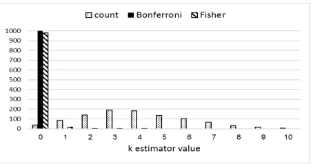
ap-Figure 1:ˆkhistogram for the independent datasets
simu-lation.
propriate under other assumptions that may become relevant in future.
We next demonstrate the value of the proposed replicability analysis through toy examples with synthetic data (Section 5) as well as analysis of state-of-the-art algorithms for four major NLP ap-plications (Section 6). Our point of reference is the standard, yet statistically unjustified, counting method that sets its estimator, kˆcount, to the num-ber of datasets for which the difference between the compared algorithms is significant withp−value
≤α(i.e.kˆcount= #{i:pi ≤α}).7 5 Toy Examples
For the examples of this section we synthesize p−values to emulate a test withN = 100 hypothe-ses (domains), and setα to 0.05. We start with a simulation of a scenario where algorithmAis equiv-alent toB for each domain, and the datasets repre-senting these domains are independent. We sample the 100p−values from a standard uniform distribu-tion, which is thep−value distribution under the null hypothesis, repeating the simulation 1,000 times.
Since all the null hypotheses are true then k, the number of false null hypotheses, is 0. Fig-ure 1 presents the histogram of ˆk values from all 1,000 iterations according to ˆkBonf erroni, ˆkF isher andˆkcount.
The figure clearly demonstrates that kˆcount pro-vides an overestimation ofkwhile ˆkBonf erroni and ˆ
kF isherdo much better. Indeed, the histogram yields the following probability estimates: Pˆ(ˆkcount >
7We useαin two different contexts: the significance level of
[image:8.612.315.542.53.172.2]k) = 0.963, Pˆ(ˆkBonf erroni > k) = 0.001 and ˆ
P(ˆkF isher > k) = 0.021 (only the latter two are lower than 0.05). This simulation strongly supports the theoretical results of Section 4.2.
To consider a scenario where a dependency be-tween the participating datasets does exist, we con-sider a second toy example. In this example we gen-erateN = 100p−values corresponding to 34 inde-pendent normal test statistics, and two other groups of 33 positively correlated normal test statistics with ρ = 0.2 and ρ = 0.5, respectively. We again as-sume that all null hypotheses are true and thus all the p−values are distributed uniformly, repeating the simulation 1,000 times. To generate positively dependent p−values, we followed the process de-scribed in Section 6.1 of Benjamini et al. (2006).
We estimate the probability that ˆk > k = 0for the threeˆkestimators based on the 1000 repetitions and get the values of: Pˆ(ˆkcount > k) = 0.943,
ˆ
P(ˆkBonf erroni > k) = 0.046 and Pˆ(ˆkF isher > k) = 0.234. This simulation demonstrates the im-portance of using Bonferroni’s method rather than Fisher’s method when the datasets are dependent, even if some of the datasets are independent. 6 NLP Applications
In this section we demonstrate the potential impact of replicability analysis on the way experimental re-sults are analyzed in NLP setups. We explore four NLP applications: (a) two where the datasets are in-dependent: multi-domain dependency parsing and multilingual POS tagging; and (b) two where depen-dency between the datasets does exist: cross-domain sentiment classification and word similarity predic-tion with word embedding models.
6.1 Data
Dependency Parsing We consider a multi-domain setup, analyzing the results reported in Choi et al. (2015). The authors compared ten state-of-the-art parsers from which we pick three: (a) Mate (Bohnet, 2010)8 that performed best on
the majority of datasets; (b) Redshift (Honnibal et al., 2013)9 which demonstrated comparable, still
somewhat lower, performance compared to Mate;
8code.google.com/p/mate-tools. 9github.com/syllog1sm/Redshift.
and (c) SpaCy (Honnibal and Johnson, 2015) that was substantially outperformed by Mate.
All parsers were trained and tested on the En-glish portion of the OntoNotes 5 corpus (Weischedel et al., 2011; Pradhan et al., 2013), a large multi-genre corpus consisting of the following 7 multi-genres: broadcasting conversations (BC), broadcasting news (BN), news magazine (MZ), newswire (NW), pivot text (PT), telephone conversations (TC) and web text (WB). Train and test set size (in sentences) range from 6672 to 34,492 and from 280 to 2327, respec-tively (see Table 1 of Choi et al. (2015)). We copy the test set UAS results of Choi et al. (2015) and computep−values using the data downloaded from http://amandastent.com/dependable/.
POS Tagging We consider a multilingual setup, analyzing the results reported in (Pinter et al., 2017). The authors compare their MIMICK model with the model of Ling et al. (2015), denoted with CHAR→TAG. Evaluation is performed on 23 of the 44 languages shared by the Polyglot word embed-ding dataset (Al-Rfou et al., 2013) and the univer-sal dependencies (UD) dataset (De Marneffe et al., 2014). Pinter et al. (2017) choose their languages so that they reflect a variety of typological, and partic-ularly morphological, properties. The training/test split is the standard UD split. We copy the word level accuracy figures of Pinter et al. (2017) for the low resource training set setup, the focus setup of that paper. The authors kindly sent us theirp-values.
Sentiment Classification In this task, an algo-rithm is trained on reviews from one domain and should classify the sentiment of reviews from an-other domain to the positive and negative classes. For replicability analysis we explore the results of Ziser and Reichart (2017) for the cross-domain sen-timent classification task of Blitzer et al. (2007). The data in this task consists of Amazon product reviews from 4 domains: books (B), DVDs (D), electronic items (E), and kitchen appliances (K), for the total of 12 domain pairs, each domain having a 2000 re-view test set.10 Ziser and Reichart (2017) compared
the accuracy of their AE-SCL-SR model to MSDA (Chen et al., 2011), a well known domain adaptation
10http://www.cs.jhu.edu/˜mdredze/
method, and kindly sent us the requiredp-values.
Word Similarity We compare two state-of-the-art word embedding collections: (a) word2vec CBOW (Mikolov et al., 2013) vectors, generated by the model titled the best “predict” model in Baroni et al. (2014);11 and (b) GloVe (Pennington et al., 2014)
vectors generated by a model trained on a 42B to-ken common web crawl.12 We employed the demo
of Faruqui and Dyer (2014) to perform a Spearman correlation evaluation of these vector collections on 12 English word pair datasets: WS-353 (Finkelstein et al., 2001b), WS-353-SIM (Agirre et al., 2009), WS-353-REL (Agirre et al., 2009), MC-30 (Miller and Charles, 1991), RG-65 (Rubenstein and Good-enough, 1965), Rare-Word (Luong et al., 2013), MEN (Bruni et al., 2012), MTurk-287 (Radinsky et al., 2011), MTurk-771 (Halawi et al., 2012), YP-130 (Yang and Powers, ), SimLex-999 (Hill et al., 2016), and Verb-143 (Baker et al., 2014).
6.2 Statistical Significance Tests
We first calculate the p−values for each task and dataset according to the principals ofp−values com-putation for NLP as discussed in Yeh (2000), Berg-Kirkpatrick et al. (2012) and Søgaard et al. (2014).
For dependency parsing, we employ the a-parametric paired bootstrap test (Efron and Tibshi-rani, 1994) that does not assume any distribution on the test statistics. We chose this test because the dis-tribution of the values for the measures commonly applied in this task is unknown. We implemented the test as in (Berg-Kirkpatrick et al., 2012) with a bootstrap size of 500 and with105repetitions.
For multilingual POS tagging, we employ the Wilcoxon signed-rank test (Wilcoxon, 1945) on the differences of the sentence level accuracy scores of the two compared models. This test is a non-parametric test for differences in measure, testing the null hypothesis that the difference has a sym-metric distribution around zero. It is appropriate for tasks with paired continuous measures for each ob-servation, which is the case when comparing sen-tence level accuracies.
11http://clic.cimec.unitn.it/composes/
semantic-vectors.html. Parameters: 5-word context window, 10 negative samples, subsampling, 400 dimensions.
12http://nlp.stanford.edu/projects/glove/. 300 dimensions.
For sentiment classification we employ the Mc-Nemar test for paired nominal data (McMc-Nemar, 1947). This test is appropriate for binary classifi-cation tasks and since we compare the results of the algorithms when applied on the same datasets, we employ its paired version. Finally, for word simi-larity with its Spearman correlation evaluation, we choose the Steiger test (Steiger, 1980) for compar-ing elements in a correlation matrix.
We consider the case ofα= 0.05for all four ap-plications. For the dependent datasets experiments (sentiment classification and word similarity predic-tion) with their generally lower p−values (see be-low), we also consider the case whereα= 0.01.
[image:10.612.314.540.359.613.2]6.3 Results
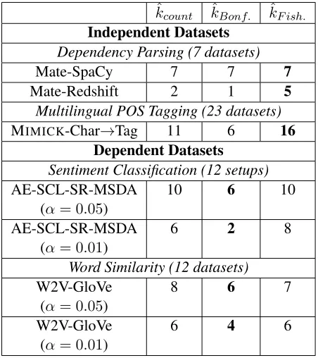
Table 1 summarizes the replicability analysis results while Table 2 – 5 present task specific performance measures andp−values.
ˆ
kcount ˆkBonf. ˆkF ish.
Independent Datasets
Dependency Parsing (7 datasets)
Mate-SpaCy 7 7 7
Mate-Redshift 2 1 5
Multilingual POS Tagging (23 datasets)
MIMICK-Char→Tag 11 6 16 Dependent Datasets
Sentiment Classification (12 setups)
AE-SCL-SR-MSDA 10 6 10
(α= 0.05)
AE-SCL-SR-MSDA 6 2 8
(α= 0.01)
Word Similarity (12 datasets)
W2V-GloVe 8 6 7
(α= 0.05)
W2V-GloVe 6 4 6
(α= 0.01)
Table 1: Replicability analysis results. The appropriate estimator for each scenario is in bold. For independent datasetsα= 0.05.ˆkcountis based on the current practice in the NLP literature and does not have statistical guar-antees regarding overestimation of the truek. Likewise,
ˆ
Model|Data BC BN MZ NW PT TC WB
Mate 90.73 90.82 91.92 91.68 96.64 89.87 89.89
SpaCy 89.05 89.31 89.29 89.52 95.27 87.65 87.40
p−val (Mate,SpaCy) (10−4) (10−4) (0.0) (0.0) (2·10−4) (9·10−4) (0.0)
Redshift 90.19 90.46 90.90 90.99 96.22 88.99 89.31
[image:11.612.64.547.53.139.2]p−val (Mate,Redshift) (0.0979) (0.1662) (0.0046) (0.0376) (0.0969) (0.0912) (0.0823)
Table 2: UAS results for multi-domain dependency parsing.p−values are in parentheses.
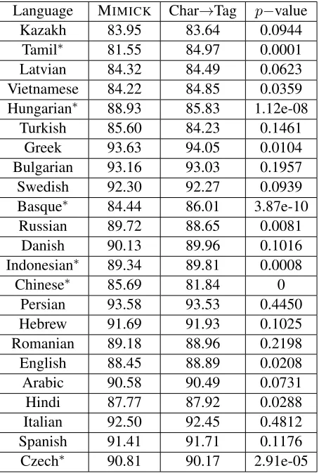
Language MIMICK Char→Tag p−value Kazakh 83.95 83.64 0.0944
Tamil∗ 81.55 84.97 0.0001 Latvian 84.32 84.49 0.0623 Vietnamese 84.22 84.85 0.0359 Hungarian∗ 88.93 85.83 1.12e-08
Turkish 85.60 84.23 0.1461 Greek 93.63 94.05 0.0104 Bulgarian 93.16 93.03 0.1957 Swedish 92.30 92.27 0.0939 Basque∗ 84.44 86.01 3.87e-10
Russian 89.72 88.65 0.0081 Danish 90.13 89.96 0.1016 Indonesian∗ 89.34 89.81 0.0008
[image:11.612.74.301.177.514.2]Chinese∗ 85.69 81.84 0 Persian 93.58 93.53 0.4450 Hebrew 91.69 91.93 0.1025 Romanian 89.18 88.96 0.2198 English 88.45 88.89 0.0208 Arabic 90.58 90.49 0.0731 Hindi 87.77 87.92 0.0288 Italian 92.50 92.45 0.4812 Spanish 91.41 91.71 0.1176 Czech∗ 90.81 90.17 2.91e-05
Table 3: Multilingual POS tagging accuracy for the MIM-ICK and the Char→Tag models. ∗ indicates languages identified by the Holm procedure withα= 0.05.
Independent Datasets Dependency parsing (Ta-ble 2) and multilingual POS tagging (Ta(Ta-ble 3) are our example tasks for this setup, where ˆkF isher is our recommended valid estimator for the number of cases where one algorithm outperforms another.
For dependency parsing, we compare two scenar-ios: (a) where in most domains the differences be-tween the compared algorithms are quite large and thep−values are small (Mate vs. SpaCy); and (b)
Dataset AE-SCL-SR MSDA p−value B→K 0.8005 0.788 0.0268 B→D∗ 0.8105 0.783 0.0011 B→E 0.7675 0.7455 0.0119 K →B∗ 0.7295 0.7 0.0038 K →D∗,+ 0.763 0.714 1.9e-06
K→E 0.84 0.824 0.018
[image:11.612.313.540.178.361.2]D→B 0.773 0.7605 0.0186 D→K∗ 0.8025 0.774 0.0014 D→E∗ 0.781 0.75 0.0011 E→B 0.7115 0.7185 0.4823 E→K 0.8455 0.845 0.9507 E →D∗,+ 0.745 0.71 0.0003
Table 4: Cross-domain sentiment classification accuracy for models taken from (Ziser and Reichart, 2017). In an
X →Y setup,Xis the source domain andY is the target
domain.∗and+indicate domains identified by the Holm
procedure withα= 0.05andα= 0.01, respectively.
where in most domains the differences between the compared algorithms are smaller and thep−values are higher (Mate vs. Redshift). Our multilingual POS tagging scenario (MIMICKvs. Char→Tag) is more similar to scenario (b) in terms of the differ-ences between the participating algorithms.
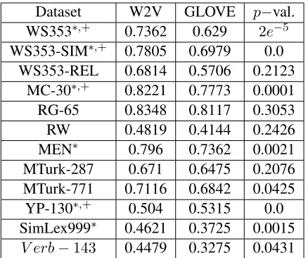
Dataset W2V GLOVE p−val. WS353∗,+ 0.7362 0.629 2e−5
WS353-SIM∗,+ 0.7805 0.6979 0.0
WS353-REL 0.6814 0.5706 0.2123 MC-30∗,+ 0.8221 0.7773 0.0001
RG-65 0.8348 0.8117 0.3053 RW 0.4819 0.4144 0.2426 MEN∗ 0.796 0.7362 0.0021 MTurk-287 0.671 0.6475 0.2076 MTurk-771 0.7116 0.6842 0.0425 YP-130∗,+ 0.504 0.5315 0.0
[image:12.612.77.296.53.236.2]SimLex999∗ 0.4621 0.3725 0.0015 V erb−143 0.4479 0.3275 0.0431
Table 5: Spearman’sρvalues for the best performing pre-dict model (W2V-CBOW) of (Baroni et al., 2014) and the GLOVE model.∗and+are as in Table 4.
tagging results are similar to case (b) of dependency parsing. Here, again,ˆkcountis too conservative, es-timating the number of languages with effect to be 11 (out of 23) whileˆkF isher estimates this number to be 16 (an increase of 5/23 in the estimated num-ber of languages with effect). kˆ
Bonf erroniis again more conservative, estimating the number of lan-guages with effect to be only 6, which is not very surprising given that it does not exploit the indepen-dence between the datasets. These two examples of case (b) demonstrate that when the differences be-tween the algorithms are quite small, kˆ
F isher may be more sensitive than the current practice in NLP for discovering the number of datasets with effect.
To complete the analysis, we would like to name the datasets with effect. As discussed in Section 4.2, while this can be straightforwardly done by naming the datasets with the ˆk smallestp−values, in gen-eral, this approach does not control the probability of identifying at least one dataset erroneously. We thus employ the Holm procedure for the identification task, noticing that the number of datasets it identi-fies should be equal to the value of thekˆBonf erroni estimator (Section 4.3).
Indeed, for dependency parsing in case (a), the Holm procedure identifies all seven domains as cases where Mate outperforms SpaCy, while in case (b) it identifies only the MZ domain as a case where Mate outperforms Redshift. For multilingual POS
tagging the Holm procedure identifies Tamil, Hun-garian, Basque, Indonesian, Chinese and Czech as languages where MIMICK outperforms Char→Tag. This analysis demonstrates that when the perfor-mance gap between two algorithms becomes nar-rower, inquiring for more information (i.e. identify-ing the domains with effect rather than just estimat-ing their number), may result in weaker results.13
Dependent Datasets In cross-domain sentiment classification (Table 4) and word similarity predic-tion (Table 5), the involved datasets manifest mu-tual dependence. Particularly, each sentiment setup shares its test dataset with 2 other setups, while in word similarity WS-353 is the union of WS-353-REL and WS-353-SIM. As discussed in Section 4, ˆ
kBonf erroniis the appropriate estimator of the num-ber of cases one algorithm outperforms another.
The results in Table 1 manifest the phenomenon demonstrated by the second toy example in Sec-tion 5, which shows that when the datasets are de-pendent, ˆkF isher as well as the error-prone ˆkcount may be too optimistic regarding the number of datasets with effect. This stands in contrast to ˆ
kBonf erroni which controls the probability to over-estimate the number of such datasets.
Indeed, ˆkBonf erroni is much more conservative, yielding values of 6 (α = 0.05) and 2 (α = 0.01) for sentiment, and of 6 (α = 0.05) and 4 (α = 0.01) for word similarity. The differences from the conclusions that might have been drawn by ˆkcount are again quite substantial. The difference between ˆ
kBonf erroniandkˆcountin sentiment classification is 4, which accounts to 1/3 of the 12 test setups. Even for word similarity, the difference between the two methods, which account to 2 for bothαvalues, rep-resents 1/6 of the 12 test setups. The domains identi-fied by the Holm procedure are marked in the tables.
Results Overview Our goal in this section is to demonstrate that the approach of simply looking at the number of datasets for which the difference be-tween the performance of the algorithms reaches a predefined significance level, gives different results
13For completeness, we also performed the analysis for the
independent dataset setups with α = 0.01. The results are (kˆcount,ˆkBonf erroni,kˆF isher): Mate vs. SpaCy: (7,7,7); Mate
from our suggested statistically sound analysis. This approach is denoted here withˆk
count and shown to be statistically not valid in Sections 3.2 and 5. We observe that this happens especially in evaluation se-tups where the differences between the algorithms are small for most datasets. In some cases, when the datasets are independent, our analysis has the power to declare a larger number of datasets with effect than the number of individual significant test values (kˆcount). In other cases, when the datasets are interdependent,kˆ
countis much too optimistic. Our proposed analysis changes the observations that might have been made based on the papers where the results analyzed here were originally re-ported. For example, for the Mate-Redshift com-parison (independent evaluation sets), we show that there is evidence that the number of datasets with effect is much higher than one would assume based on counting the significant sets (5 vs. 2 out of 7 evaluation sets), giving a stronger claim regarding the superiority of Mate. In multilingual POS tag-ging (again, a setup of independent evaluation sets) our analysis shows evidence for 16 sets with ef-fect compared to only 11 of the erroneous count method - a difference in 5 out of 23 evaluation sets (21.7%). Finally, in the cross-domain sentiment classification and the word similarity judgment tasks (dependent evaluation sets), the unjustified counting method may be too optimistic (e.g. 10 vs. 6 out of 12 evaluation sets, for α = 0.05 in the sentiment task), in favor of the new algorithms.
7 Discussion and Future Directions
We proposed a statistically sound replicability anal-ysis framework for cases where algorithms are com-pared across multiple datasets. Our main contribu-tions are: (a) analyzing the limitacontribu-tions of the current practice in NLP work; and (b) proposing a frame-work that addresses both the estimation of the num-ber of datasets with effect and their identification.
The framework we propose addresses two differ-ent situations encountered in NLP: independdiffer-ent and dependent datasets. For dependent datasets, we as-sumed that the type of dependency cannot be deter-mined. One could use more powerful methods if cer-tain assumptions on the dependency between the test statistics could be made. For example, one could use
the partial conjunction p-value based on Simes test for the global null hypothesis (Simes, 1986), which was proposed by Benjamini and Heller (2008) for the case where the test statistics satisfy certain posi-tive dependency properties (see Theorem 1 in (Ben-jamini and Heller, 2008)). Using this partial con-junction p-value rather than the one based on Bon-ferroni, one may obtain higher values ofkˆwith the same statistical guarantee. Similarly, for the iden-tification question, if certain positive dependency properties hold, Holm’s procedure could be replaced by Hochberg’s or Hommel’s procedures (Hochberg, 1988; Hommel, 1988) which are more powerful.
An alternative, more powerful multiple testing procedure for identification of datasets with effect, is the method in Benjamini and Hochberg (1995), that controls the false discovery rate (FDR), a less strict error criterion than the one considered here. This method is more appropriate in cases where one may tolerate some errors as long as the proportion of er-rors among all the claims made is small, as expected to happen when the number of datasets grows.
We note that the increase in the number of evalua-tion datasets may have positive and negative aspects. As noted in Section 2, we believe that multiple com-parisons are integral to NLP research when aiming to develop algorithms that perform well across lan-guages and domains. On the other hand, exper-imenting with multiple evaluation sets that reflect very similar linguistic phenomena may only compli-cate the comparison between alternative algorithms. In fact, our analysis is useful mostly where the datasets are heterogeneous, coming from different languages or domains. When they are just techni-cally different but could potentially be just combined into a one big dataset, then we believe the ques-tion of Demˇsar (2006), whether at least one dataset shows evidence for effect, is more appropriate. Acknowledgement
References
Eneko Agirre, Enrique Alfonseca, Keith Hall, Jana Kravalova, Marius Pas¸ca, and Aitor Soroa. 2009. A study on similarity and relatedness using distributional and WordNet-based approaches. In Proceedings of HLT-NAACL.
Rami Al-Rfou, Bryan Perozzi, and Steven Skiena. 2013. Polyglot: Distributed word representations for multi-lingual NLP. InProceedings of CoNLL.
Simon Baker, Roi Reichart, and Anna Korhonen. 2014. An unsupervised model for instance level subcatego-rization acquisition. InProceedings of EMNLP. Marco Baroni, Georgiana Dinu, and Germ´an Kruszewski.
2014. Don’t count, predict! a systematic compari-son of context-counting vs. context-predicting seman-tic vectors. InProceedings of ACL.
C. Glenn Begley and Lee M. Ellis. 2012. Drug develop-ment: Raise standards for preclinical cancer research.
Nature, 483(7391):531–533.
Yoav Benjamini and Ruth Heller. 2008. Screen-ing for partial conjunction hypotheses. Biometrics, 64(4):1215–1222.
Yoav Benjamini and Yosef Hochberg. 1995. Control-ling the false discovery rate: A practical and powerful approach to multiple testing. Journal of the Royal Sta-tistical Society. Series B (Methodological), pages 289– 300.
Yoav Benjamini, Abba M. Krieger, and Daniel Yekutieli. 2006. Adaptive linear step-up procedures that control the false discovery rate. Biometrika, pages 491–507. Yoav Benjamini, Ruth Heller, and Daniel Yekutieli.
2009. Selective inference in complex research. Philo-sophical Transactions of the Royal Society of London A: Mathematical, Physical and Engineering Sciences, 367(1906):4255–4271.
Taylor Berg-Kirkpatrick, David Burkett, and Dan Klein. 2012. An empirical investigation of statistical signifi-cance in NLP. InProceedings of EMNLP-CoNLL. John Blitzer, Ryan McDonald, and Fernando Pereira.
2006. Domain adaptation with structural correspon-dence learning. InProceedings of EMNLP.
John Blitzer, Mark Dredze, and Fernando Pereira. 2007. Biographies, Bollywood, boom-boxes and blenders: Domain adaptation for sentiment classification. In
Proceedings of ACL.
Bernd Bohnet. 2010. Very high accuracy and fast depen-dency parsing is not a contradiction. InProceedings of COLING.
Elia Bruni, Gemma Boleda, Marco Baroni, and Nam-Khanh Tran. 2012. Distributional semantics in tech-nicolor. InProceedings of ACL.
Elia Bruni, Nam-Khanh Tran, and Marco Baroni. 2014. Multimodal distributional semantics. Journal of Arti-ficial Intelligence Research (JAIR), 49:1–47.
Sabine Buchholz and Erwin Marsi. 2006. CoNLL-x shared task on multilingual dependency parsing. In
Proceedings of CoNLL.
Yee Seng Chan and Hwee Tou Ng. 2007. Domain adap-tation with active learning for word sense disambigua-tion. InProceedings of ACL.
Eugene Charniak. 2000. A maximum-entropy-inspired parser. InProceedings of HLT-NAACL.
Minmin Chen, Yixin Chen, and Kilian Q. Weinberger. 2011. Automatic feature decomposition for single view co-training. InProceedings of ICML.
Jinho D. Choi, Joel Tetreault, and Amanda Stent. 2015. It depends: Dependency parser comparison using a web-based evaluation tool. InProceedings of ACL. Open Science Collaboration. 2012. An open,
large-scale, collaborative effort to estimate the reproducibil-ity of psychological science. Perspectives on Psycho-logical Science, 7(6):657–660.
Michael Collins. 2003. Head-driven statistical models for natural language parsing. Computational linguis-tics, 29(4):589–637.
Hal Daum´e III. 2007. Frustratingly easy domain adapta-tion. InProceedings of ACL.
Marie-Catherine De Marneffe, Timothy Dozat, Natalia Silveira, Katri Haverinen, Filip Ginter, Joakim Nivre, and Christopher D. Manning. 2014. Stanford depen-dencies: A cross-linguistic typology. InProceedings of LREC.
Janez Demˇsar. 2006. Statistical comparisons of clas-sifiers over multiple data sets. Journal of Machine Learning Research, 7:1–30.
Thomas G. Dietterich. 1998. Approximate statistical tests for comparing supervised classification learning algorithms.Neural computation, 10(7):1895–1923. Bradley Efron and Robert J. Tibshirani. 1994. An
intro-duction to the bootstrap. CRC press.
Alessio Farcomeni. 2007. A review of modern multiple hypothesis testing, with particular attention to the false discovery proportion. Statistical Methods in Medical Research.
Manaal Faruqui and Chris Dyer. 2014. Community evaluation and exchange of word vectors at wordvec-tors.org. InProceedings of the ACL: System Demon-strations.
Lev Finkelstein, Evgeniy Gabrilovich, Yossi Matias, Ehud Rivlin, Zach Solan, Gadi Wolfman, and Eytan Ruppin. 2001a. Placing search in context: The con-cept revisited. InProceedings of WWW.
Ruppin. 2001b. Placing search in context: The con-cept revisited. InProceedings of WWW.
Honglei Guo, Huijia Zhu, Zhili Guo, Xiaoxun Zhang, Xian Wu, and Zhong Su. 2009. Domain adapta-tion with latent semantic associaadapta-tion for named entity recognition. InProceedings of HLT-NAACL.
Guy Halawi, Gideon Dror, Evgeniy Gabrilovich, and Yehuda Koren. 2012. Large-scale learning of word relatedness with constraints. InProceedings of ACM SIGKDD.
Ruth Heller, Marina Bogomolov, and Yoav Benjamini. 2014. Deciding whether follow-up studies have repli-cated findings in a preliminary large-scale omics study.
Proceedings of the National Academy of Sciences, 111(46):16262–16267.
Thomas Herndon, Michael Ash, and Robert Pollin. 2014. Does high public debt consistently stifle economic growth? a critique of Reinhart and Rogoff. Cambridge Journal of Economics, 38(2):257–279.
Felix Hill, Roi Reichart, and Anna Korhonen. 2015. Simlex-999: Evaluating semantic models with (gen-uine) similarity estimation. Computational Linguis-tics, 41(4):665–695.
Felix Hill, Roi Reichart, and Anna Korhonen. 2016. Simlex-999: Evaluating semantic models with (gen-uine) similarity estimation. Computational Linguis-tics.
Yosef Hochberg. 1988. A sharper Bonferroni proce-dure for multiple tests of significance. Biometrika, 75(4):800–802.
Sture Holm. 1979. A simple sequentially rejective multi-ple test procedure. Scandinavian Journal of Statistics, 6(2):65–70.
Gerhard Hommel. 1988. A stagewise rejective multi-ple test procedure based on a modified Bonferroni test.
Biometrika, 75(2):383–386.
Matthew Honnibal and Mark Johnson. 2015. An im-proved non-monotonic transition system for depen-dency parsing. InProceedings of EMNLP.
Matthew Honnibal, Yoav Goldberg, and Mark Johnson. 2013. A non-monotonic arc-eager transition system for dependency parsing. InProceedings of CoNLL. Philipp Koehn and Josh Schroeder. 2007. Experiments in
domain adaptation for statistical machine translation. InProceedings of the Second Workshop on Statistical Machine Translation.
Philipp Koehn. 2005. Europarl: A parallel corpus for statistical machine translation. InProceedings of the tenth Machine Translation Summit.
Jeffrey T. Leek and Roger D Peng. 2015. Opinion: Reproducible research can still be wrong: Adopting a prevention approach. Proceedings of the National Academy of Sciences, 112(6):1645–1646.
Omer Levy and Yoav Goldberg. 2014. Dependency-based word embeddings. InProceedings of ACL. Wang Ling, Chris Dyer, Alan W. Black, Isabel Trancoso,
Ramon Fermandez, Silvio Amir, Luis Marujo, and Tiago Luis. 2015. Finding function in form: Com-positional character models for open vocabulary word representation. InProceedings of EMNLP.
Thomas M. Loughin. 2004. A systematic compari-son of methods for combining p-values from indepen-dent tests. Computational Statistics & Data Analysis, 47(3):467–485.
Minh-Thang Luong, Richard Socher, and Christopher D. Manning. 2013. Better word representations with re-cursive neural networks for morphology. In Proceed-ings of CoNLL.
Mitchell P. Marcus, Mary Ann Marcinkiewicz, and Beat-rice Santorini. 1993. Building a large annotated cor-pus of English: The Penn Treebank. Computational linguistics, 19(2):313–330.
Edison Marrese-Taylor and Yutaka Matsuo. 2017. Repli-cation issues in syntax-based aspect extraction for opinion mining. In Proceedings of the Student Re-search Workshop at EACL.
Quinn McNemar. 1947. Note on the sampling error of the difference between correlated proportions or per-centages. Psychometrika, 12(2):153–157.
Tomas Mikolov, Ilya Sutskever, Kai Chen, Gregory S. Corrado, and Jeffrey Dean. 2013. Distributed rep-resentations of words and phrases and their composi-tionality. InProceedings of NIPS.
George A. Miller and Walter G. Charles. 1991. Contex-tual correlates of semantic similarity. Language and cognitive processes, 6(1):1–28.
Ramal Moonesinghe, Muin J. Khoury, and A. Cecile J. W. Janssens. 2007. Most published research find-ings are false but a little replication goes a long way.
PLoS Med, 4(2):e28.
Aur´elie N´ev´eol, Cyril Grouin, Kevin Bretonnel Cohen, and Aude Robert. 2016. Replicability of research in biomedical natural language processing: a pilot evalu-ation for a coding task. Proceedings of EMNLP. Jens Nilsson, Sebastian Riedel, and Deniz Yuret. 2007.
The CoNLL 2007 shared task on dependency parsing. InProceedings of CoNLL.
Diarmuid ´O S´eaghdha and Anna Korhonen. 2014. Prob-abilistic distributional semantics. Computational Lin-guistics, 40(3):587–631.
Prasad Patil, Roger D. Peng, and Jeffrey Leek. 2016. A statistical definition for reproducibility and replicabil-ity.bioRxiv.
Jeffrey Pennington, Richard Socher, and Christopher Manning. 2014. GloVe: Global vectors for word rep-resentation. InProceedings of EMNLP.
Slav Petrov and Ryan McDonald. 2012. Overview of the 2012 shared task on parsing the web. In Notes of the First Workshop on Syntactic Analysis of Non-Canonical Language (SANCL).
Yuval Pinter, Robert Guthrie, and Jacob Eisenstein. 2017. Mimicking word embeddings using subword RNNs. InProceedings of EMNLP.
Sameer Pradhan, Alessandro Moschitti, Nianwen Xue, Hwee Tou Ng, Anders Bj¨orkelund, Olga Uryupina, Yuchen Zhang, and Zhi Zhong. 2013. Towards robust linguistic analysis using OntoNotes. InProceedings of CoNLL.
Kira Radinsky, Eugene Agichtein, Evgeniy Gabrilovich, and Shaul Markovitch. 2011. A word at a time: Com-puting word relatedness using temporal semantic anal-ysis. InProceedings of WWW.
Herbert Rubenstein and John B. Goodenough. 1965. Contextual correlates of synonymy. Communications of the ACM, 8(10):627–633.
Roy Schwartz, Roi Reichart, and Ari Rappoport. 2015. Symmetric pattern based word embeddings for im-proved word similarity prediction. InProceedings of CoNLL.
Carina Silberer and Mirella Lapata. 2014. Learning grounded meaning representations with autoencoders. InProceedings of ACL.
R. John Simes. 1986. An improved Bonferroni proce-dure for multiple tests of significance. Biometrika, pages 751–754.
Rion Snow, Brendan O’Connor, Daniel Jurafsky, and Andrew Y. Ng. 2008. Cheap and fast—but is it good?: Evaluating non-expert annotations for natural language tasks. InProceedings of EMNLP.
Anders Søgaard, Anders Johannsen, Barbara Plank, Dirk Hovy, and H´ector Mart´ınez Alonso. 2014. What’s in a p-value in NLP ? InProceedings of CoNLL. Anders Søgaard. 2013. Estimating effect size across
datasets. InProceedings of HLT-NAACL.
James H. Steiger. 1980. Tests for comparing ele-ments of a correlation matrix. Psychological Bulletin, 87(2):245–251.
Ralph Weischedel, Eduard Hovy, Mitchell Marcus, Martha Palmer, Robert Belvin, Sameer Pradhan, Lance Ramshaw, and Nianwen Xue. 2011. OntoNotes: A large training corpus for enhanced pro-cessing. Handbook of Natural Language Processing and Machine Translation. Springer.
Frank Wilcoxon. 1945. Individual comparisons by rank-ing methods. Biometrics bulletin, 1(6):80–83.
Dongqiang Yang and David M.W. Powers. Verb similar-ity on the taxonomy of WordNet. InProceedings of the 3rd International WordNet Conference.
Alexander Yeh. 2000. More accurate tests for the statis-tical significance of result differences. InProceedings of CoNLL.
Yftah Ziser and Roi Reichart. 2017. Neural structural correspondence learning for domain adaptation. In