A Bootstrap Stationarity Test for Predictive
Regression Invalidity
∗
Iliyan Georgiev
a, David I. Harvey
b, Stephen J. Leybourne
band A.M. Robert Taylor
caDepartment of Statistical Sciences, University of Bologna
bSchool of Economics, University of Nottingham
cEssex Business School, University of Essex
Abstract
In order for predictive regression tests to deliver asymptotically valid inference, account has to be taken of the degree of persistence of the predictors under test. There is also a maintained assumption that any predictability in the variable of interest is purely attributable to the predictors under test. Violation of this assumption by the omission of relevant persistent predictors renders the predictive regression invalid with the result that both the finite sample and asymptotic size of the predictability tests can be significantly inflated, with the potential therefore to spuriously indicate predictability. In response we propose a predictive regression invalidity test based on a stationarity testing approach. To allow for an unknown degree of persistence in the putative predictors, and for heteroskedasticity in the data, we implement our proposed test using a fixed regressor wild bootstrap procedure. We demonstrate the asymptotic validity of the proposed bootstrap test. This entails demonstrating that the asymptotic distribution of the bootstrap statistic, conditional on the data, is the same (to first-order) as the asymptotic null distribution of the statistic computed on the original data, conditional on the predictor. This corrects a long-standing error in the bootstrap literature whereby it is incorrectly argued that for strongly persistent regressors the validity of the fixed regressor bootstrap obtains through equivalence to an unconditional limit distribution. Our bootstrap results are therefore of interest in their own right and are likely to have important applications beyond the present context. An illustration is given by re-examining the results relating to U.S. stock returns data in Campbell and Yogo (2006).
Keywords: Predictive regression; Granger causality; persistence; stationarity test; fixed regressor wild bootstrap; conditional distribution.
JEL Classification: C12, C32.
∗We are grateful to the Editor, Todd Clark, an anonymous Co-Editor and three anonymous referees
for their helpful and constructive comments. We particularly thank one of the referees for suggesting the examples relating to latent predictors discussed in section 2. Correspondence to: Robert Taylor, Essex Business School, University of Essex, Wivenhoe Park, Colchester, CO4 3SQ, United Kingdom. Email:
1
Introduction
Predictive regression (hereafter PR) is a widely used tool in applied finance and economics,
and forms the basis for Granger causality testing. A very common application is in the
con-text of testing the linear rational expectations hypothesis. A core example of this is testing
whether future (excess) stock returns are predictable (Granger caused) by current
infor-mation, such as the dividend yield or the term structure of interest rates. Often it is found
that the posited predictor variable (e.g. dividend yield) exhibits persistence behaviour akin
to a (near) unit root autoregressive process, whilst the variable being predicted (e.g. the
stock return) resembles a (near) martingale difference sequence [m.d.s.].
In basic form, a test of predictability involves running an OLS regression of the variable
being predicted, yt say, on the lagged value of a posited predictor variable, xt say, and
testing the significance of the estimated coefficient on xt−1 using a standard regression t
-ratio. Here the null hypothesis is thatytis unpredictable (in mean) and, hence, a m.d.s.; the
alternative is that it is predictable from xt−1 (i.e. that xt−1 Granger causes yt). Cavanagh
et al. (1995) [CES] show that when the innovation driving xt is correlated with yt (as is
often thought to be case in practice; e.g., the stock price is a component of both the return
and the dividend yield), then these tests can be badly over-sized if xtis a local to unit root
process but critical values appropriate for the case where xt is a pure unit root process are
used. This over-size can be interpreted as a tendency towards finding spurious predictability
in yt, in that it is incorrectly concluded that xt−1 can be used to predict yt when in fact
yt is unpredictable; see also Rossi (2005) for a discussion of related issues. Attempting to
address this issue, CES discuss Bonferroni bound-based procedures that yield conservative
tests, while Campbell and Yogo (2006) [CY] consider a point optimal variant of the t-test
and employ confidence belts. Phillips (2014) proposes a modification to the test proposed
in CY which is asymptotically valid in the case where xt can be either local-to-unity or
stationary. Recently, Breitung and Demetrescu (2015) [BD] consider variable addition and
instrumental variable (IV) methods to correct test size. Near-optimal PR tests can also be
found in Elliott et al. (2015) and Jansson and Moreira (2006).
A misspecified PR of yt on xt−1 (with non-zero slope) can also arise from these tests
{xt} and) by some other persistent process, {zt} say. The variable zt might be a manifest
variable or an unobserved latent variable. Here, and in the extreme case where yt and
the past of xt are independent, such that xt−1 is an invalid predictor variable, it is known
that the regression ofyt onxt−1 can lead to serious upward size distortions in the standard
PR tests, with the same conclusion of spurious predictability of yt by xt−1 as discussed
earlier; see Ferson et al. (2003a,b) and Deng (2014). More generally, where xt and zt are
correlated such that yt and the past of xt are no longer independent, a linear predictor
of yt by xt−1 would still be misspecified because it would be suboptimal with respect to
quadratic loss, even if the optimal linear predictor based on observables might involve xt−1.
Specifically, where zt is a latent variable correlated with xt, xt−1 would pick up some of
the information from the past of zt and so even in the case of Granger non-causality1 of
yt by the process {xt}, xt−1 would not be a spurious predictor variable; nevertheless, the
optimal linear predictor of yt would involve further variables among the lags of yt and
xt−1. Where zt is manifest, the optimal linear predictor for yt would involve the past of
zt. This fundamental misspecification problem in the estimated PR will affect all of the
predictability tests discussed above.
We demonstrate theoretically and by means of simulations the potential for a
misspec-ified PR of yt on xt−1 to arise in the context of a model where xt and zt follow persistent
processes, which we model as local-to-unity autoregressions, while modelling the coefficient
on zt−1 as being local-to-zero. As a consequence, it is important to be able to identify,
a priori, if yt is Granger caused by some ignored {zt}. Our approach involves testing
for persistence in the residuals from a regression of yt on xt−1. Consequently, any effect
that xt−1 may have on yt, through the value of its slope coefficient in the putative PR, is
eliminated from the residuals, and any persistence they display thereafter is attributable
to the unincluded variable zt−1, and would signal that the PR is misspecified. The test
for PR misspecification we suggest is based on the co-integration tests of Shin (1994) and
Leybourne and McCabe (1994), themselves variants of the stationarity test of Kwiatkowski
et al. (1992) [KPSS]. Although originally designed to detect pure unit root behaviour in
re-1We distinguish between Granger causality, defined by conditioning on counterfactual information sets
that can be chosen to contain the past of the variablez, observable or not, and predictability as a pragmatic
gression residuals, M¨uller (2005) shows these tests also reject when near unit root behaviour
is present, making them well-suited to the testing scenario of this paper.
An issue arising with our proposed test is that under its null hypothesis thatzt−1 plays
no role in the data generating process [DGP] for yt, its limit distribution depends on the
local-to-unity parameter in the process for xt, even though the residuals used are invariant
to the coefficient on xt−1 in the DGP. In principle, this makes it difficult to control the size
of the test. However, we show a bootstrap procedure which treats xt−1 as a fixed regressor
(i.e. the observed xt−1 is used in calculating bootstrap analogues of our test statistic) can
be implemented to yield an asymptotically size-controlled test. This fixed regressor
boot-strap approach is not itself new to the literature and has been employed by, among others,
Gon¸calves and Kilian (2004) and Hansen (2000). Because many financial and economic
time series are thought to display non-stationary volatility and/or conditional
heteroskedas-ticity in their innovations, it is also important for our proposed testing procedure to be
(asymptotically) robust to these effects. We therefore use a heteroskedasticity-robust
vari-ant of the fixed regressor bootstrap along the lines proposed in Hansen (2000). This uses
a wild bootstrap scheme to generate bootstrap analogues of yt. We show that our
pro-posed fixed regressor wild bootstrap test has local asymptotic power against the same local
alternatives that give rise to a misspecified PR of yt on xt−1.
We establish large sample validity of our bootstrap method by showing that the
asymp-totic distribution of the bootstrap statistic, conditional on the data, is the same (to
first-order) as the asymptotic null distribution of the statistic computed on the original data,
conditional on the posited predictor variable. Our proof corrects a long-standing error in
the bootstrap literature arising from Hansen (2000) who incorrectly suggests, in the context
of a different test statistic, that for strongly persistent regressors the validity of the fixed
regressor bootstrap follows from the coincidence of the unconditional limiting distribution
of the original statistic with that of the limiting distribution of the bootstrap statistic
con-ditional of the data. We show that this coincidence does not occur for strongly persistent
regressors. The results we provide have wider applicability to other scenarios where a fixed
regressor bootstrap is used with (near-) integrated regressors.
the various null and alternative hypotheses regarding predictability ofyt byxt−1 andzt−1.
To aid lucidity, we consider a single putative predictor variable, xt, and single unincluded
variable, zt, both with m.d.s. errors. Generalisations to richer model specifications are
straightforward and discussed at various points. Section 3 details the asymptotic
distribu-tions of standard PR statistics under the various hypotheses, demonstrating the inference
problems caused by unincluded persistent variables. Section 4 introduces our proposed test
for PR invalidity, detailing its limit distribution and showing the validity of the fixed
re-gressor wild bootstrap scheme in providing asymptotic size control. The asymptotic power
of this procedure is also examined here and compared with the degree of size distortions
associated with PR tests. Section 5 presents the results of a set of finite sample simulations
investigating the size and power of our proposed bootstrap tests. An empirical illustration
reconsidering the results pertaining to U.S stock returns data in CY is given in Section 6.
Proofs and additional simulation results appear in a supplementary appendix.
We use the following notation: b·c is the floor function; I(·) is the indicator function;
x := y (x =: y) means that x is defined by y (y is defined by x); →w and →p for weak
convergence and convergence in probability, respectively. For a vector, x, kxk := (x0x)1/2, the Euclidean norm. Finally, Dk :=D
k[0,1] is the space of right continuous with left limit
(c`adl`ag) functions from [0,1] toRk, equipped with the Skorokhod topology, andD :=D1.
2
The Model and Predictability Hypotheses
The basic DGP we consider for observed yt is
yt=αy+βxxt−1+βzzt−1+yt, t = 1, ..., T (1)
where xt and zt satisfy
xt =αx+sx,t, zt=αz+sz,t, t= 0, ..., T (2)
sx,t =ρxsx,t−1+xt, sz,t=ρzsz,t−1+zt, t= 1, ..., T (3)
whereρx:= 1−cxT−1andρz := 1−czT−1, withcx ≥0 andcz ≥0, so thatxtandztare unit
root or local-to-unit root autoregressive processes. We let sx,0 and sz,0 be Op(1) variates.
we discuss, we parameterise βx and βz asβx =gxT−1 and βz =gzT−1, respectively, which
entails that when gx and/orgz are non-zero, yt is a persistent, but local-to-noise process.2
Our interest lies in examining the behaviour of predictability tests derived from the PR
of yt on xt−1 when yt is generated by the DGP in (1)-(3) with βz 6= 0, and subsequently
developing tests for the null hypothesis that βz = 0. In doing so, it is important to note
that the motivating issue of spurious predictability of yt by xt−1, in the case where there
is no correlation between xt−1 and zt−1, arises whenever xt−1 and the unincluded zt−1 are
both persistent processes. In the general case where no dependence restrictions are placed
between xt−1 and zt−1, the presence of zt−1 in (1) does not entail that xt−1 is a spurious
predictor for yt. Rather it implies that the PR of yt on xt−1 alone is misspecified.
In the context of (1),zt−1 could be either an omitted manifest variable or an unobserved
latent variable. An example of the latter is given by the case where yt are (currency,
commodity or bond) returns and xt−1 is either the lagged forward premium (spot minus
forward price/rate) or a lagged futures basis (spot minus futures price/rate). Here there is
an unobserved latent risk premium which is believed to be strongly persistent, and which in
combination with the strongly persistent predictor has been suggested as a possible driver
for empirically unorthodox findings, such as the well known forward premium (or Fama)
puzzle; see Gospodinov (2009). A second example is provided by the long-run risk model
of Bansal and Yaron (2004). Certain versions of their model can be re-written as PRs for
returns with an unobserved long-run persistent component in consumption. In the latent
case it would also be quite reasonable to view zt not through a literal interpretation of the
DGP in (1)-(3) but rather as a general proxy for underlying misspecification in the PR,
under which interpretation it would clearly not make sense for zt to be stationary rather
than persistent. Possible examples are provided by the case where the coefficient on xt−1
displays time-varying behaviour, such as has been considered in, for example, Paye and
Timmermann (2006) and Cai et al. (2015), or where the data on xt are observed with a
strongly persistent measurement error driven by relatively low variance innovations.
2Notice that an observationally equivalent formulation of the model can be obtained by treating β
x
and βz as fixed constants but parameterising the variances of xt and zt to be local-to-zero; see, in
particular, the discussion following equation (10) later. We choose the local-to-zero coefficient formulation
The innovation vectort := [xt, zt, yt]0 is taken to satisfy the following conditions:
Assumption 1. The innovation process t can be written as t=HDtet where:
(a) H and Dt are the 3×3 non-stochastic matrices
H :=
h11 0 0
h21 h22 0
h31 h32 h33
, Dt :=
d1t 0 0
0 d2t 0
0 0 d3t
with hij ∈R, hii >0 (i, j = 1,2,3), and HH0 strictly positive definite. The volatility terms
dit satisfy dit=di(t/T), where di ∈ D are non-stochastic, strictly positive functions.
(b) et is a 3×1vector martingale difference sequence [m.d.s.] with respect to a filtration
Ft,to which it is adapted, with conditional covariance matrix σt:=E(ete0t|Ft−1)satisfying:
(i) T−1PT t=1σt
p
→E(ete0t) =I3; (ii) suptEketk4+δ <∞ for some δ >0.
Remark 1. Assumption 1 implies thatt is a vector m.d.s. relative toFt, with conditional
variance matrix Ωt|t−1 :=E(t0t|Ft−1) = (HDt)σt(HDt)0, and time-varying unconditional
variance matrix Ωt :=E(tt0) = (HDt)(HDt)0. Stationary conditional heteroskedasticity
and non-stationary unconditional volatility are obtained as special cases with Dt = I3
(constant unconditional variance, hence only conditional heteroskedasticity) and σt = I3
(so Ωt|t−1 = Ωt = Ω(t/T), only unconditional non-stationary volatility), respectively.3
As discussed in Cavaliere, Rahbek and Taylor (2010), Assumption 1(a) implies that the
elements of Ωtare only required to be bounded and to display a countable number of jumps,
therefore allowing for an extremely wide class of potential models for the behaviour of the
variance matrix of t, including single or multiple variance or covariance shifts, variances
which follow a broken trend, and smooth transition variance shifts.
Remark 2. Under Assumption 1, an identification issue regarding the parametersβx, βz
and h21 arises in the case where cx = cz. In this case, whenever the observables (yt, xt)
satisfy (1) for certain βx, βz 6= 0 andzt,they also satisfy (1) for βλx =βx+λ, β λ
z =βz, and
zλ
t =zt−λβ−z1xt, for any λ, where ztλ is also a (local-to-) unit root autoregressive process
and its innovations λzt = zt − λβ
−1
z xt are such that [xt, λzt, yt]0 satisfies Assumption
1, upon a redefinition of the matrix H. In particular, if βz 6= 0, then it is possible to
3The assumption thatE(e
te0t) =I3made in part (b)(i) and the parameterisation of the unconditionally
choose λ =h21h−111βz such that xt and λzt, the innovations driving xt and ztλ respectively,
are uncorrelated. In accordance with OLS identification conditions, we will discuss the
predictive implications of (1) under the identifying condition E(xtzt) = 0 (equivalently,
h21 = 0) if βz 6= 0, and under the condition βz = 0 otherwise. In the case where zt is a
named latent variable (such as an unobserved risk premium) or a manifest variable, the
value of E(xtzt) is implicitly fixed by the choice of zt and an alternative is to discuss (1)
by taking this value into consideration.
Remark 3. We notice that a PR based on xt−1 alone is misspecified whenever βz 6= 0,
regardless of the value of either βx or the correlation between xt and zt. If h21 = 0, xt−1
and zt−1 would be uncorrelated with one another and any conclusion of predictability from
the PR of yt onxt−1 in the case where βx= 0 and βz 6= 0 in (1) would be purely spurious
because the best linear predictor (with respect to symmetric quadratic loss) [BLP] of yt
given the past of{yt, xt}would not involvext−1, although the BLP with respect to a larger
information set might involve xt−1. When h21 6= 0, xt−1 and zt−1 are correlated, and thus,
for forecasting purposes, xt−1 could act as a proxy for the information in zt−1. Nonetheless,
if βz 6= 0, the BLP of yt would not be a function of xt−1 alone: for a manifest variable zt,
the BLP given the past of {yt, xt, zt} would involve zt−1, whereas for a latent variable zt,
the BLP given the past of {yt, xt} would involve yt−1 (and, in general, also xt−1 even if
βx = 0, as some of the predictive power available from zt−1 would be picked up by xt−1).
Remark 4. For transparency, the structure in (1)- (3) is exposited for a scalar variable,zt.
This is without loss of generality, as one may consider that zt =γ0zt∗ where z
∗
t is a vector
of variables, which might therefore contain both omitted manifest and latent variables.
We are now ready to discuss, in the context of (1), the possibilities for the predictability
and causation of yt by the variables xt−1 and zt−1, focusing on linear predictors. One
potential case that has received much attention in the literature is that whereytis
Granger-caused only by the process{xt}, so that it is predictable only byxt−1, implying thatβx 6= 0
while βz = 0 in (1). This forms the alternative hypothesis in the PR tests discussed in
section 3, where the corresponding null is thatβx = 0, and, in the context of our model, the
maintained hypothesis that βz = 0, so that yt is unpredictable under the null. However,
the PR. In this case, βx = 0 andβz 6= 0, thereby violating the aforementioned maintained
hypothesis, and a PR of yt on xt−1 alone would be misspecified, regardless of whether zt
is a manifest or latent variable (see Remark 3). In the special case where h21 = 0 and
xt−1 does not enter the BLP of yt, a conclusion to the contrary is an instance of spurious
predictability. A final possibility is that βx 6= 0 andβz 6= 0 so thatytis Granger-caused by
both processes{xt}and{zt}. In this last case ifzt was an omitted manifest variable then a
correctly specified PR could be obtained by including zt−1 in the PR. If, on the other hand,
zt was a latent variable, a correctly specified BLP of yt would include more observables
(e.g., yt−1) than xt−1. We summarize these four cases using the following taxonomy of
hypotheses within the context of DGP (1):
Hu : βx = 0, βz = 0 yt is unpredictable (in mean)
Hx : βx 6= 0, βz = 0 yt is Granger-caused by {xt} alone
Hz : βx = 0, βz = 06 yt is Granger-caused by {zt} alone
Hxz : βx 6= 0, βz 6= 0 yt is Granger-caused by {xt} and {zt}
In hypothesis testing terms, standard PR tests attempt to distinguish between the null
Hu and the alternativeHx. Here, we consider the impact of the presence ofzt−1 in the DGP
on such tests, that is we investigate the behaviour of PR tests of Hu against Hx when in
fact Hz orHxz is true. In addition, we propose a test for possible PR invalidity, where the
appropriate composite null isHu orHx (Hu,Hx), and the alternative Hz orHzx (Hz,Hzx).
We end this section by stating some implications of Assumption 1 for our asymptotic
analysis. Associated to a standard Brownian motion B = [B1, B2, B3]0 in R3, let Bη =
[Bη1, Bη2, Bη3]0 be the heteroskedastic Gaussian motion defined byBηi(r) := f
−1/2 i
Rr
0 di(s)dBi(s),
r ∈ [0,1], where fi :=
R1 0 di(s)
2ds, i = 1,2,3. We can also write B ηi
d
= Bi(ηi), i = 1,2,3,
where ηi denotes the variance profile ηi(r) := fi−1R0rdi(s)2ds, r ∈ [0,1], such that Bηi is
a time-changed Brownian motion; see, for example, Davidson (1994, p.486). In particular,
ηi(r) =r, r ∈[0,1], under unconditional homoskedasticity. Then the following functional
weak convergence result holds in D3×
R3×3, by Lemma 1 of Boswijk et al. (2016):
T−1/2
bT rc
X
t=1
t, T−1 T
X
t=1 t−1
X
s=1
s0t
!
w
→
Mη(r),
Z 1
0
Mη(s)dMη(s)0
where Mη := [Mηx, Mηz, Mηy]0 := HF1/2Bη for the diagonal matrix F := diag{f1, f2, f3}.
Let Ωη := {ωab}a,b∈{x,y,z} := V ar{Mη(1)} = HF H0, which in the unconditionally
ho-moskedastic case Dt=I3 reduces to
HH0 =
h2
11 h11h21 h11h31
h11h21 h221+h222 h21h31+h22h32
h11h31 h21h31+h22h32 h231+h232+h233
=:
σxx σxz σxy
σxz σzz σzy
σxy σzy σyy
=: Ω.
It will prove convenient to define the two Ornstein-Uhlenbeck-type processes Mηc,u(r) :=
Rr
0e
(s−r)cudM
ηu(s) for u = x, z and r ∈ [0,1], along with the standardised analogues
Bηc,u(r) :=ω
−1/2
uu Mηc,u(r) and their demeaned counterparts ¯Bηc,u(r) :=Bηc,u(r)−
R1
0Bηc,u(s).
3
Asymptotic Behaviour of Predictive Regression Tests
To fix ideas, as in CES, we first consider the basic PR test of Hu againstHx, based on the
t-ratio for testing βx = 0 in the fitted linear regression
yt = ˆαy+ ˆβxxt−1+ ˆyt, t= 1, ..., T. (5)
The test statistic is given by
tu :=
ˆ βx q s2 y/ PT
t=1(xt−1−x−¯ 1)2
, βˆx :=
PT
t=1(xt−1−x−¯ 1)yt
PT
t=1(xt−1−x¯−1)2
and s2y := (T −2)−1PT
t=1ˆ 2
yt , with ¯x−1 :=T−1
PT
t=1xt−1.
In addition to thet-test, we also analyze a point optimal variant introduced by CY. For
a known value of ρx, the (infeasible) test statistic takes the following form:
Q:=
ˆ
βx−(sxy/s2x)(ˆρx−ρx)
q
s2
y{1−(s2xy/s2ys2x)}/
PT
t=1(xt−1 −x¯−1)2
where ˆβx and s2
y are as defined above, sxy := (T − 2)−1PTt=1ˆxtˆyt and s2x := (T −
2)−1PT
t=1ˆ 2
xt with ˆxt denoting the OLS residuals from regressing xt on a constant and
xt−1, and where ˆρx :=
PT
t=1(xt−1−x−¯ 1)xt/
PT
t=1(xt−1−x−¯ 1)2. In the case where sxy = 0,
Q and tu coincide.
Theorem 1. For the DGP (1), (2), (3) and under Assumption 1, the weak limits of tu
and Q as T → ∞ are of the form
R1
0M¯ηc,x(r)dNηy(r)
q R1
0M¯ηc,x(r)2
+ gx
R1
0M¯ηc,x(r) 2+g
z
R1
0M¯ηc,x(r)Mηc,z(r)
q
ny
R1
0M¯ηc,x(r)2
(6)
where M¯ηc,x(r) := Mηc,x(r)−
R1
0Mηc,x(s)ds, r ∈ [0,1], and Nηy, ny are statistic-specific.
Thus, for the tu statistic, Nηy := ω
−1/2
yy Mηy and ny := ωyy, whereas for the Q statistic,
Nηy :=ω
−1/2
y|x {Mηy −ωxyω
−1
xxMηx} and ny :=ωyy−ω2xy/ωxx =:ωy|x.
Remark 5. Notice that the limit expressions for tu and Q in (6) are identical when
h31 = 0 (i.e. ωxy = 0). The limit expression in (6) shows the dependence of tu and Q on
gz underHz (wheregx= 0 but gz 6= 0). Consequently, even for infeasible versions of these
tests where all other nuisance parameters were known, the use of asymptotic critical values
appropriate for these tests under Hu will not result in size-controlled procedures underHz
and raises the possibility that spurious rejections in favour of predictability of yt by xt−1
will be encountered when yt is actually predictable by zt−1 (cf. Ferson et al., 2003a,b, and
Deng, 2014, for related results under non-localized βz). Under Hxz, where both gx 6= 0
and gz 6= 0, any rejection by tu or Q could not uniquely be ascribed to the role of xt−1,
potentially suggesting the existence of a well-specified PR that is in fact under-specified
due to the omission of zt−1. The same issues also hold for the feasible versions of the tu
and Q tests developed in CES and in CY and Phillips (2014), respectively.
Remark 6. In the special case where cx =cz, the limit of tu in (6) can be written as
R1
0B¯ηc,x(r)dMηy(r)
q
ωyy
R1
0B¯ηc,x(r)2
+g⊥x(ωxx ωyy
)1/2
q R1
0B¯ηc,x(r)2+gz(
ωz|x
ωyy
)1/2
R1
0B¯ηc,x(r)Bηc,2(r)
q R1
0B¯ηc,x(r)2
(7)
with Bηc,2(r) :=
Rr
0 e
(s−r)czdB
η2(s) for r ∈ [0,1], ωz|x := ωzz − ω2xz/ωxx and g⊥xT
−1 :=
(gx+ωxzω−xx1gz)T−1 representing the coefficient of xt−1 in a redefinition of (1) where xt−1
is orthogonal to the unincluded persistent variable (see Remark 2 with λ = h21h−111βz =
ωxzω−xx1gzT−1). Not surprisingly, therefore, tu can be anticipated to have relatively low
power to reject Hu in favour of Hxz when the contribution of xt−1 to the variability of yt
(as measured by |g⊥x|ω1xx/2ωyy−1/2) is low, and also the contribution of zt−1 corrected for xt−1
(as measured by |gz|ω 1/2 z|xω
−1/2
(for h316= 0) renders the leading term in (7) non-Gaussian, affecting both the size and the
power of the test. These comments also apply to the limit of the Q statistic, except that
the first term in (7) is standard Gaussian.
We will now proceed to investigate the extent of the size distortions that occur in the
tu and Q tests when gz 6= 0. Before doing so, it should be noted that other PR tests have
been proposed in the literature, including the near-optimal tests of Elliottet al. (2015) and
Jansson and Moreira (2006); see the useful recent summaries provided in BD and Caiet al.
(2015). The issues we discuss in this paper are pertinent irrespective of which particular
PR test one uses, in cases where the putative and unincluded predictors are persistent.
They are also relevant for the case where a putative PR contains multiple predictors.
3.1
Asymptotic Size of Predictive Regression Tests under
H
zTo obtain as transparent as possible a picture of the large sample size properties of tu and
QunderHz we abstract from any role that non-stationary volatility plays by settingdi = 1,
i= 1,2,3. We then simulate the limit distributions using 10,000 Monte Carlo replications,
approximating the Brownian motion processes in the limiting functionals for (6) using
independentN(0,1) random variates, with the integrals approximated by normalized sums
of 2,000 steps. Critical values are obtained by setting gx = gz = 0; for tu these depend
on cx and also (it can be shown) h231/(h231+h322 +h233) = σ2xy/σxxσyy, while for Q, these
depend on cx alone. These quantities are assumed known, so we are essentially analyzing
the large sample behaviour of infeasible variants of tu andQ. We graph nominal 0.10-level
sizes of two-sided tests as functions of the parameter gz ={0,2.5,5.0, ...50.0} with gx = 0.
For cx = cz = c = {0,10}we set σxx = σzz = σyy = 1, and consider σxy = σzy = 0 plus
σxy = −0.70 with σzy = {0,−0.70,0.70} where σxz = 0 throughout. Setting cx = cz is
not a requirement here, but simply facilitates keeping xt and zt balanced in terms of their
persistence properties.
The results of this size simulation exercise are shown in Figure 1. Forc= 0 we observe
the sizes of tu andQ growing monotonically from the baseline 0.10 level with increasinggz,
thereby giving rise to an ever-increasing likelihood of ascribing spurious predictive ability
as small as gz = 12.5 produces sizes in excess of 0.50. The size patterns for tu and Q
are also quite similar, which is as we would expect given that gz impacts upon their limit
distributions in a very similar way. Of course, whenσxy = 0, the tests have identical limits,
while for σxy =−0.7, there is a general tendency for Q to show slightly more pronounced
over-sizing thantu (possibly reflecting the relatively higher power that this test can achieve
underHx). Size distortions appear little influenced by the value taken byσzy. Withc= 10
qualitatively, the same comments apply here as for the case c = 0. That said, we do
observe that the over-sizing now manifests itself more slowly with increasing gz. Indeed,
when σzy = −0.70 some modest under-size is observed for small values of gz. However,
both sizes are still above 0.50 oncegz = 50 so spurious predictability does remain a serious
issue. That the problem is less severe here simply reflects the fact that xt−1 and zt−1 are
lower (but still high) persistence processes.
It would be difficult to argue that spurious predictive ability is not a potentially
impor-tant consideration to take into account when employing either of thetu andQtests to infer
predictability with high persistence processes. Although we have focussed this analysis on
OLS-based PR tests, similar qualitative results will pertain for other PR tests including
the recently proposed IV-based tests of BD whenever a high persistence IV is used. A low
persistence IV test should be less prone to over-size in the presence of a high persistence
unincluded predictor zt−1, but the price paid for employing such an IV is that when a
true predictor xt−1 is high persistence, the IV test will have very poor power. Basically,
whenever there is scope for high persistence properties of regressors to yield good power
for PR tests, we should always remain alert to the possibility of spurious predictability.
4
A Test for Predictive Regression Invalidity
Given the potential for standard PR tests to spuriously signal predictability of yt by xt−1
(alone) when βz 6= 0, we now consider a test devised to distinguish between βz = 0 and
βz 6= 0. Non-rejection by such a test would indicate that zt−1 plays no role in predicting
yt, and hence that standard PR tests based on xt−1 are valid. Rejection, however, would
indicate the presence of an unincluded variable zt−1 in the DGP for yt, signalling the
that βz = 0, i.e. Hu,Hx, against the alternative thatβz 6= 0, i.e. Hz,Hxz, in (1).
4.1
The Test Statistic and Conventional Asymptotics
The test we develop is based on testing a null hypothesis of stationarity; specifically, we
adapt the co-integration tests of Shin (1994) and Leybourne and McCabe (1994), which
are themselves variants of the KPSS test. We employ the statistic
S :=s−2T−2
T
X
t=1 t
X
i=1
ˆ ei
!2
(8)
where s2 := (T −3)−1PT
t=1eˆ 2
t and ˆet are the OLS residuals from the fitted regression
yt= ˆαy+ ˆβxxt−1+ ˆβ∆x∆xt+ ˆet, t = 1, ..., T (9)
where, as in Shin (1994), the regressor ∆xt is included in (9) to account for the possibility
of correlation betweenxt andyt (h316= 0). Abstracting from the role of the regressor ∆xt,
whenβz 6= 0, the residuals ˆetincorporate a contribution of the unincludedzt−1 term in (1),
hence the persistence in zt−1 is passed to ˆet, and the statisticS is a test of βz = 0 against
βz 6= 0, rejecting for large values of S. Specifically, assuming cz = 0, we can rewrite (1) as
yt =αy +βxxt−1+rt−1+yt (10)
wherert =rt−1+ut, initialised atr0 =βzαz (on setting sz,0 = 0 with no loss of generality)
with innovations ut = βzzt. Testing the null of βz = 0 against βz =gzT−1 in (1) is then
seen to be precisely the same problem as testing the null of V(ut) =:σuu = 0 against σuu
=gz2T−2σzz in the context of (10), withgz = 0 under both nulls. If we temporarily assume
that xt is strictly exogenous and yt and zt are independent IID normal random variates,
then S is the locally best invariant (to αy, αx, αz, βx and σyy) test of the null σuu = 0
against the local alternative σuu = g2zT−2σzz in (10). As such, the statistic S is relevant
for our testing problem where we seek to distinguish between βz = 0 and βz 6= 0. In our
model we do not impose cz = 0 (nor the other temporary assumptions above), so in these
more general circumstances we consider S to deliver a near locally best invariant test.
Notwithstanding the foregoing motivation, it is important to stress that a test based on
such, a rejection by this test indicates that the fitted regression in (9) is not a valid PR.
As with the failure of any mis-specification test, this does not tell us why the regression
has failed. We do know that S delivers a test which is (approximately) locally optimal in
the direction of zt−1 being an unincluded variable (be it manifest or latent), but a rejection
does not mean that xt−1 is not a valid predictor for yt. Therefore, our proposed test is
one for the invalidity of the putative PR, not of the putative predictor, xt−1; see again the
discussion on this point in section 2.
In Theorem 2 we now detail the limiting distribution of S under Assumption 1.
Theorem 2. For the DGP (1), (2), (3) and under Assumption 1,
S →w R1
0{F(r, cx) +gzG(r, cx, cz)} 2
dr (11)
where
F(r, cx) := Bη,y|x(r)−
Rr
0B¯ηc,x(s){
R1
0B¯ηc,x(s) 2}−1R1
0B¯ηc,x(s)dBη,y|x(s),
G(r, cx, cz) := (
ωzz
ωy|x
)1/2
( Z r
0
¯
Bηc,z(s)−
R1
0 B¯ηc,x(s)Bηc,z(s)
R1
0 B¯ηc,x2 (s)
Z r
0
¯ Bηc,x(s)
)
with ωy|x := ωyy −ω2xy/ωxx, Bη,y|x(r) := Bη,y|x(r) −rBη,y|x(1), r ∈ [0,1], and Bη,y|x :=
ω−y|1x/2{Mηy −ωxyω−xx1Mηx} a standardised heteroskedastic Brownian motion independent of
B1.
Remark 7. Notice that the limit in (11) does not depend onh31owing to the invariance of
the residuals ˆet to this parameter arising from the presence of the regressor ∆xt in (9). In
the special casecx =cz, the limit is also invariant to h21 (cf. Remark 2). In fact, asMηz =
ωxzω−xx1Mηx+ωz|xBη2 for ωz|x :=ωzz−ω2xz/ωxx, in this case the equality of the decay rate
in the Ornstein-Uhlenbeck processes Mηc,x andMηc,z ensures thatBηc,z|x :=ω
−1/2
z|x {Mηc,z−
ωxzω−xx1Mηc,x} equals the Ornstein-Uhlenbeck process Bηc,2 soG(r, cx, cz) reduces to
G(r, cx, cx) =
ωz|x
ωy|x
1/2(Z r
0
¯
Bηc,2(s)−
R1
0 B¯ηc,x(s)Bηc,2(s)
R1
0 B¯2ηc,x(s)
Z r
0
¯ Bηc,x(s)
)
.
The term gzG(r, cx, cz) in (11) is key in enabling the test S to potentially distinguish
betweenHu,Hx andHz,Hxz. Clearly ifωz|x/ωy|x '0, then such a test has low power. This
that is not shared and therefore not removed by the regressor xt−1, on average over t), or
more generally, when zt corrected for xt varies little relatively to yt corrected forxt. For
cx 6=cz the limit ofSdepends onh21asG(r, cx, cx)−G(r, cx, cz) is proportional toh21h−111.
Remark 8. Under Hu,Hx, where gz = 0, the limit distribution of S in (11) simplifies to
R1
0F(r, cx)
2and depends only onc
x and any unconditional heteroskedasticity present int.
Remark 9. We have assumed thus far that the xt are serially uncorrelated, with et
being an m.d.s. More generally we may consider a linear process assumption for xt of the
form xt =
P∞
i=0θivx,t−i where vx,t is the first element of HDtet and with the conditions
P∞
i=0i|θi| < ∞ and
P∞
i=0θi 6= 0 satisfied. Under homoskedasticity, this would include
all stationary and invertible ARMA processes. Notice that yt remains uncorrelated with
the increments of xt at all lags (i.e. xt is weakly exogenous with respect to yt) under this
structure. In this case, it may be shown that the limiting results given in Theorem 2 above
and in Theorems 3-5 below continue to hold provided we replace (9) in the calculation of
S with the augmented variant
yt = ˆαy+ ˆβxxt−1+ ˆβ∆x∆xt+ p
X
i=1
ˆδi∆xt−i+ ˆet, t =p+ 1, ..., T (12)
where p satisfies the standard rate condition that 1/p+p3/T → 0, as T → ∞, and it is
assumed thatT1/2P∞
i=p+1|δi| →0, where{δi}
∞
i=1 are the coefficients of theAR(∞) process
obtained by inverting the M A(∞) for xt. Similarly to BD, we would also need to restrict
the amount of serial dependence allowed in the conditional variances via the assumption
that supi,j≥1kτijk < ∞, where τij := E(ete0t⊗et−ie0t−j), with ⊗ denoting the Kronecker
product. Serial correlation of a similar form in zt will have no impact on our large sample
results under the null hypothesis, Hu,Hx, although an effect does arise underHz,Hxz. As is
standard in the PR literature, we maintain the assumption thatytis serially uncorrelated.
Remark 10. Extensions to the case where the putative PR contains multiple regressors
and/or more general deterministic components can easily be handled in the context of our
proposed PR invalidity test. Specifically, denoting the deterministic component as τ0ft,
where ft is as defined in section 3.2 of BD, an obvious example being the linear trend case
where ft := (1, t)0, and the vector of putative regressors as xt−1, then we would need to
correspondingly construct S using the residuals from the regression of yt on ft, xt−1 and
in the sequel, but would not alter the primary conclusion given in Corollary 1 below, that
the fixed regressor wild bootstrap implementation of this test is asymptotically valid.
A consequence of the result in Theorem 2 is therefore that if we wish to base a test
for PR invalidity on S, then we need to address the fact that under the null Hu,Hx the
limit distribution of S is not pivotal. In order to account for the dependence of inference
on any unconditional heteroskedasticity present, we employ a wild bootstrap procedure
based on the residuals ˆet. However, we also need to account for the dependence of the
limit distribution of S on cx, and this we carry out by using the observed outcome on
x:= [x0, ..., xT]0 as a fixed regressor in the bootstrap procedure which we detail next.
4.2
A Fixed Regressor Wild Bootstrap Stationarity Test
A standard approach to obtaining bootstrap critical values for S would involve repeated
generation of bootstrap samples for the original yt, such that they mimic (in a statistical
sense) the behaviour ofytwith the null Hu, Hx imposed, together with repeated generation
of bootstrap samples for the original xt, to mimic the behaviour ofxt. For each bootstrap
sample, these would then be used to calculate a bootstrap analogue of S, which should
then reflect the behaviour of S under the null. Generation of bootstrap samples ofyt with
suitable properties is quite straightforward, at least in large samples, using a standard wild
bootstrap re-sampling scheme from the residuals ˆet from (9). However, finding bootstrap
samples of xt presents a significant problem since xt = (1−cxT−1)xt−1 +xt (assuming
αx = 0 for simplicity) and so any corresponding recursion used to construct bootstrap
samples for xt from bootstrap samples of ext requires, for a size-controlled test, that cx
should be known or consistently estimated. Unfortunately, it is well-known that consistent
estimation of cx is not feasible. To avoid this problem, we circumvent estimation of cx
altogether and instead follow the approach taken in Hansen (2000), considering a bootstrap
procedure which uses xas a fixed regressor; that is, the bootstrap statistic S∗ is calculated from the same observed xt as was used in the construction of S itself.
We now outline the steps involved in our proposed fixed regressor wild bootstrap.
(i) Construct the wild bootstrap innovations y∗t := ˆetwt, where wt, t = 1, . . . , T, is an
IID N(0,1) sequence independent of the data and ˆetare the residuals from either (9)
or (12).
(ii) Calculate the fixed regressor wild bootstrap analogue of S,
S∗ := (s∗y)−2T−2
T
X
t=1 t
X
i=1
ˆ∗yi
!2
where (s∗y)2 := (T−2)−1PT
t=1(ˆ
∗
yt)2and ˆ
∗
ytare OLS residuals from the fitted regression
yt∗ = ˆα∗y+ ˆβ∗xxt−1+ ˆ∗yt, t= 1, ..., T. (13)
(iii) Define the correspondingp-value asPT∗ := 1−G∗T (S) withG∗T denoting the conditional (on the original data) cumulative distribution function (cdf) of S∗. In practice, G∗T is unknown, but can be approximated in the usual way by numerical simulation.
(iv) The wild bootstrap test of Hu, Hx at level ξ rejects in favour of Hz, Hxz if PT∗ ≤ξ.
Remark 11. The wild bootstrap scheme used to generate y∗t is constructed so as to replicate the pattern of heteroskedasticity present in the original innovations; this follows
because, conditionally on ˆet, yt∗ is independent over time with zero mean and variance ˆe2t.
Remark 12. By definition, the residuals ˆetfrom (9) are invariant to the value ofβx in (1),
and so we can assume thatβx = 0 with no loss of generality when generating the bootstrap
y∗t data. We also do not include ∆xt as an additional regressor (or lags thereof in the case
considered in Remark 9) in (13). This is because the ˆetused to constructy∗t are free of any
effects arising from correlation between xt and yt, or from any weak dependence in xt.
Remark 13. Although ˆet depends on gz under Hz,Hxz, we show in the next subsection
that this does not translate into large sample dependence of S∗ ongz.
4.3
Conditional Asymptotics and Bootstrap Validity
We show that the use ofxt−1 as a fixed regressor in the construction of the bootstrap
Assumption 1 and any of the hypotheses Hu, Hx, Hz and Hxz the distribution ofS∗, given
the data, converges weakly to the random distribution which obtains by conditioning the
limit in (11) corresponding to gz = 0, on the weak limit B1 of the process T−1/2P
bT rc
t=1 e1t,
r ∈ [0,1]. This fact (along with some regularity conditions) makes it possible to conclude
that the bootstrap p-value PT∗ is asymptotically uniform U[0,1]-distributed under Hu, Hx,
by using a general result on bootstrap validity from Cavaliere and Georgiev (2017,
Theo-rem 2). From a pragmatic perspective, such a conclusion ensures that the bootstrap test
is asymptotically sized controlled under the conditions of Assumption 1 alone.
However, under Assumption 1 alone, the shortcoming remains that the meaning of the
large-sample inference performed by our bootstrap test is unclear. Certainly, asymptotic
bootstrap inference is not unconditional becauseS∗ given the data does not converge to the unconditional limit distribution of S. On the other hand, bootstrap inference need not be
asymptotically equivalent to conditional inference onxeither. Indeed, it is well known that
Theorem 2, where the limit distribution ofSis established, cannot be taken to imply thatS
conditional on xconverges weakly to the limit in (11) conditioned onB1 (the implication is
falsified by, e.g., Example 1 of LePage, Podg´orski and Ryznar, 1997). Nevertheless, it is not
unreasonable to expect that this result holds true under certain additional requirements,
and we prove that this is in fact the case. We strengthen Assumption 1, so that under
Hu, Hx the distribution of the statistic S conditional on x converges weakly to the same
random distribution as S∗ given the data, which allows us to establish that our bootstrap test in large samples has the meaning as a test conditional on x.
The results we present differ from those given in Hansen (2000) who considers a joint
structural stability test on the constant and slope parameters in a general regression
set-ting; our test of βz = 0 for the PR in (5) can be seen as the corresponding individual test
for stability of just the intercept. Hansen argues that, under his Assumption 2, the fixed
regressor (wild) bootstrap asymptotically implements unconditional inference (see
Theo-rems 5 and 6, Hansen, 2000) and that the convergence PT∗ →w U[0,1] of bootstrapp−values under the null hypothesis follows from the equivalence of the unconditional limiting null
distribution of the original statistic and the limiting distribution of the bootstrap statistic
that any such claim about unconditional inference is not correct, at least for the non-empty
class of models satisfying both Hansen’s and our assumptions. Nonetheless the stated
con-vergence of bootstrap p-values is correct, albeit for a different reason. A fuller treatment
of this specific issue is given in Georgiev et al. (2016).
Theorem 2 is based on the invariance principle given in (4). Conditional and bootstrap
analogues of that theorem can be based on a conditional joint invariance principle for the
original and the bootstrap data. In order to obtain this result, we will need to strengthen
Assumption 1 as follows:
Assumption 2. Let Assumption 1 hold, together with the following conditions:
(a) et is drawn from a doubly infinite strictly stationary and ergodic sequence {et}∞t=−∞ which is a martingale difference w.r.t. its own past.
(b) {[e2t, e3t]}∞t=−∞ is an m.d.s. also w.r.t. X ∨ Ft, where X and Ft are the σ-algebras
generated by {e1t}∞t=−∞ and {[e2s, e3s]}ts=−∞, respectively, and X ∨ Ft denotes the smallest
σ-algebra containing both X and Ft.
(c) The initial values sx,0 and sz,0 are measurable w.r.t. X (in particular, they could be
fixed constants).
Remark 14. Arguably, the most restrictive condition in Assumption 2 is given in part (b).
A first leading example where it is satisfied is that of a symmetric multivariate GARCH
process with neither leverage nor asymmetric clustering. Specifically, letet = Ω 1/2
t εt, where
Ωt is measurable with respect to the past [ε21s, ε22s, ε23s]0, s≤t−1, and{εt}∞t=−∞ is an i.i.d. sequence such thatE(εit|ε1t, ε22t, ε32t) = 0,i= 2,3. IfEketk<∞, then it could be seen that
E(eit|X ∨Ft−1) = 0,i= 2,3. Another example is that of a multivariate stochastic volatility
processet =H 1/2
t εtwith{Ht}∞t=−∞independent of{εt}∞t=−∞and where{εt}∞t=−∞is an i.i.d. sequence with E(εit|ε1t) = 0, i= 2,3 (which is certainly true if εt is multivariate standard
Gaussian, as is usually assumed in the stochastic volatility framework). If Eketk < ∞,
then againE(eit|X ∨ Ft−1) = 0, i= 2,3. These two examples are also the leading examples
given in the univariate context by Deo (2000), and in section 3 of Gon¸calves and Kilian
(2004). It would be interesting, although beyond the scope of our paper, to investigate how
Assumption 2(b) could be weakened to the case where {et} could be well approximated
conclusions of Theorem 5 below would remain valid if Assumption 2(b) was replaced by
the condition that supt≥1E{E(Pt
s=1eis|X)}
2 <∞, i= 2,3.
In Theorem 3 we now establish three things: first, a conditional invariance principle
that can be assembled from results and ideas disseminated throughout the probabilistic
lit-erature (see, in particular, Awad, 1981, Rubshtein, 1996), second, a bootstrap extension of
that result, and third, associated convergence results for stochastic integrals. For
simplic-ity, a one-dimensional bootstrap partial-sum process is considered; it is constructed from
quantities ˜eT t that we shall subsequently specify to be the residuals ˆet from the regression
in (9). Analogously to the definition of x, let y:= [y1, ..., yT]0 and z := [z0, ..., zT]0.
Theorem 3. Let ˜eT t (t = 1, ..., T) be scalar measurable functions of x, y, z and such that
PbT rc
t=1 e˜ 2 T t
p
→Rr
0 m
2(s)ds forr∈[0,1], where m is a square-integrable real function on[0,1].
Introduce ˜tb :=wte˜T t (t = 1, ..., T), and B˜η(r) :=
Rr
0m(s)dB˜1(s), r∈ [0,1], where B˜1 is a
standard Brownian motion independent of B. Under Assumption 2, the following converge
jointly as T → ∞:
T−1/2
bT rc
X
t=1
t, T−1 T
X
t=1 t−1
X
s=1
xs[yt, zt]
!
x→w
Mη(r),
Z 1
0
Mηx(s)d[Mηy(s), Mηz(s)]
B1,
r ∈[0,1], in the sense of weak convergence of random measures on D3×
R2, and
T−1/2
bT rc
X
t=1
[e1t,˜tb], T−1 T
X
t=1 t−1
X
s=1
xs˜tb
!
x, y, z→w
B1(r),B˜η(r),
Z 1
0
Mηx(s)dB˜η(s)
B1,
r ∈[0,1], in the sense of weak convergence of random measures on D2×
R.
Remark 15. Let Ex(·) := E(·|x) and E∗(·) :=E(·|x, y, z). The convergence concept used
in Theorem 3 is defined as follows. Let ζ, ζT and ξ, ξT (T ∈ N) be random elements of
the metric spaces S and T, respectively, such that ζ, ξ and B1 are defined on the same
probability space, and similarly for ζT, ξT and x, y, z. We say that ζT|x →w ζ|B1 and
ξT|x, y, z →w ξ|B1 jointly in the sense of weak convergence of random measures on S and T
if for all bounded continuous functions f :S →R and g :T →R it holds that
[Ex(f(ζT)), E
∗
(g(ξT))]0 →w [E(f(ζ)|B1), E(g(ξ)|B1)]
0
We are already in a position to establish in Theorem 4 the large sample behaviour ofS
conditional on x, and of S∗, its bootstrap analogue from Algorithm 1, conditional on the data. These two limiting distributions will be seen to coincide under the null hypothesis.
Theorem 4. Under DGP (1)-(3) and Assumption 2, the following converge jointly as
T → ∞, in the sense of weak convergence of random measures on R:
S|x→w R1
0{F(r, cx) +gzG(r, cx, cz)} 2dr
B1 (14)
S∗|x, y, z →w R1
0F(r, cx) 2dr
B1, (15)
where the processes F and G are as defined in Theorem 2.
Remark 16. A comparison of (14) and (15) shows that the bootstrap statistic S∗, con-ditional on the data, and the original statistic S, conditional on x, converge jointly to the
same random distribution when gz = 0; that is, under the null hypothesis, Hu,Hx. An
implication of this is that the bootstrap approximation is consistent in the sense that
sup
u∈R
|Px(S ≤u)−P∗(S∗ ≤u)| p
→0, (16)
given that the random cdf of R01F(r, cx)2dr
B1 is sample-path continuous. Here Px and
P∗ denote probability conditional on x and on all the data, respectively. Thus, the dis-tribution of the ‘fixed-regressor bootstrap’ statistic S∗ conditional on the data consis-tently estimates the large-sample distribution of the original statistic S conditional on
the ‘fixed regressor’ x. This result differs from the usual formulation of bootstrap
valid-ity, where two cdfs with a common non-random limit are compared; here, in contrast,
Px(S ≤u) w
→P(R01F(r, cx)2dr≤u|B1) with a non-degenerate random limit.
In Corollary 1 below we formulate the conclusion of asymptotic validity of the bootstrap
test based on S and S∗ in terms of the bootstrap p-values.
Corollary 1. Let PT∗ := P∗(S∗ > S). Under Hu, Hx and Assumption 2, PT∗|x w
→p U[0,1]
and PT∗ →w U[0,1].
An implication of Corollary 1 is that comparison of the statistic S with a ξ level
formed from B independent simulated bootstrap S∗ statistics, which we will denote by cvξ,B), results in a bootstrap test with correct asymptotic size (ξ) underHu, Hx,
condition-ally on x and unconditionally. In what follows we denote by SB the fixed regressor wild
bootstrap procedure outlined in Algorithm 1, whereby S is compared to the critical value
cvξ,B. The asymptotic local power of SB under Hz, Hxz depends on the parameter gz.
Remark 17. For the bootstrap statistic, S∗, the same limiting distribution is obtained in (15) under the alternative hypothesis, Hz,Hxz, as under the null hypothesis. In contrast,
in the case of S, a stochastic offset, arising from the term gzG(r, cx, cz), is seen in the
limiting distributions (in (14) conditionally on x, and in (11) unconditionally). Although,
for a given alternative, the asymptotic local power is different for the bootstrap test based
on S∗ and an (infeasible) test based on the unconditional limit of S and knowledge of the parametercx (the former power is a random variable depending onB1 and the latter power
is a number), we comment in Remark 18 on some qualitative similarities.
Remark 18. The limiting functional for S in (11) and (14) is dominated in probability
(both unconditionally and conditionally on B1) bygz2
R1
0G(r, cx, cz)
2drfor largeg
z and, as a
result, asymptotic local power approaches 1 as gz diverges. Nonetheless, asymptotic local
power is not monotone in |gz|. For example, in the case cx = cz, the null component
F(r, cx) in (11) and (14) involves a term in h32Bη2(r), while the alternative component
gzG(r, cx, cz) involves a term in gz
Rr
0 B¯ηc,2 (see Remark 7). Because Bη2(r) and
Rr
0 B¯ηc,2
are positively correlated, it can be shown that E{R1
0 F(r, cx)G(r, cx, cz)dr} 6= 0 forh32 6= 0,
and similarly for the conditional expectation givenB1, a.s. As a result, whenh32 6= 0, there
exist values ofgz (dependent onB1 in the conditional case) which render the expectations
of the limits in (11) and (14) (respectively unconditional and conditional on B1), smaller
than their expectations under the null hypothesis. For such gz the limit distribution under
the alternative does not first-order stochastically dominate the limit distribution under the
null, translating into power being less than size for some size levels.
4.4
Asymptotic Local Power of Stationarity Tests under
H
zWe now consider the asymptotic local power of S and SB, the latter on average over B1.
Figure 1, so we overlay this information on them. For the asymptotic power of S under
Hz we use the limit expression (11), having first obtained 0.10-level critical values from
simulating (11) undergz = 0. Since these critical values depend on knowledge ofcx,S here
is an infeasible test against which to benchmark the power ofSB. The asymptotic power of
SB is also based on the limit distribution of S under Hz but compared against a simulated
limit bootstrap critical value cvξ,B with ξ = 0.10. For each replication, this critical value
is obtained by simulating the limit (15) using B = 2000 replications, conditioning on the
simulated B1 for that Monte Carlo replication.
When c = 0, we see the power of S rising rapidly with departures from gz = 0. For
gz = 50, its power is very close to 1. Turning attention to SB, it has a very similar power
profile to that ofS; indeed, its power marginally exceeds that ofS. It is of course anticipated
from Remark 17 that SB does not have the same asymptotic local power function as S,
but the fact that its power exceeds that of S is a welcome finding as SB, unlike S, is a
feasible procedure. When c= 10 the powers ofS and SB are near identical, but at a lower
level than whenc= 0. There is also a non-monotonicity in the power profiles of S and SB,
anticipated from Remark 18, for σzy =−0.70 whengz is small, with power dipping below
size. However, for large enough gz, this anomaly disappears.4
The important comparison here is between the power ofSB (restricting attention to the
feasible procedure) and the size of tu and Q (as their size profiles are similar we only refer
to tu). When c= 0, the power of SB exceeds the size oftu, hence the invalidity of the PR
is detected with greater frequency than tu spuriously rejects in favour of predictability of
yt by xt−1. This demonstrates the capability ofSB to detect PR invalidity in cases where
the important size problems associated with tu exist. That the power of SB exceeds the
size of tu under Hz is possibly to be expected, because S is designed to detect departures
from the null of gz = 0 whereas such departures simply represent model mis-specification
in the context of the PR test tu. With c= 10, we again see that the power ofSB generally
out-strips the sizes of tu, with the size/power differences appearing even more marked than
for c= 0. Again, the only exception to this is forσzy =−0.7 when gz is small.
The Supplementary Appendix to this paper contains asymptotic power simulation
re-4We note thatS is not LBI when we allow correlation between
yt andztso this anomalous behaviour
sults for some additional parameter configurations (for which many possibilities exist). We
consider the current setup with c= 5 and c= 20 and we find that the power of SB with
c= 20 is lower than for c= 10 due to a less persistent zt−1 lessening the impact of model
misspecification. Other simulations where we allowcz to be different tocx confirm that the
main driver of power forSBisczand notcx, as would be expected. We also considerσxz 6= 0
(with cz and cx equal or different; note that we reduce the magnitudes of σxy and σzy in
some cases to ensure Ω remains positive definite). Here the interplay between SB and tu
(Q) becomes rather more complex. For example, with cz = cx, setting σxz = ±0.5 causes
the power of SB to suffer while the frequency with which tu rejects increases, while for
cz 6=cx, only small changes are observed for σxz 6= 0 compared toσxz = 0.
5
Finite Sample Size and Power under
H
zWe now evaluate the finite sample size properties of the PR tests and the size and power
of SB. For the PR tests, we consider the feasible versions of tu and Q, proposed by CES
and CY respectively, both of which rely on Bonferroni bounds to control size.5 We also
consider the IV-based test of BD that combines fractional and sine function instruments,
denoted IVcomb, comparing this with its asymptotic χ2(1) critical value. For SB we use
B = 499 replications.
To begin, we continue to abstract from heteroskedasticity and consider finite sample
DGPs for the same settings as used in the main asymptotic simulations. Specifically,
we simulate the DGP (1)-(3) for T = 200 with αy = αx = αz = 0, gx = 0, sx,0 =
sz,0 = 0, dit = 1 (i = 1,2,3), and et ∼ IID N(0, I3). Figure 2 reports the finite sample
analogues of Figure 1, i.e. rejection frequencies of nominal 0.10-level (two-sided for tu, Q
and IVcomb) tests under Hz. Simulations are again conducted using 10,000 Monte Carlo
replications. On comparing Figure 2 with its large sample counterpart Figures 1, it is
clear that our asymptotic simulations provide a close approximation to the finite sample
rejection frequencies of tu, Qand SB, particularly in terms of the relative behaviour of the
tests, albeit in absolute terms the finite sample rejection frequencies tend to be slightly
lower than their asymptotic counterparts. For tu and Q this is partly due to the feasible
tests not having the same large sample properties as the infeasible tests. The general
observations made on the basis of the asymptotic simulations apply equally here; finite
sample size of the PR tests increases with gz, giving rise to an increasing likelihood of
concluding spurious predictive ability. As anticipated in the discussion of section 3.1, a
similar pattern of rejections is found for IVcomb; its sizes are close to those of tu and Q. As
regardsSB, its finite sample power increases withgz, with the invalidity of the PR generally
being detected with greater frequency than the PR tests’ spurious rejections. Hence, the
ability of SB to detect PR invalidity in cases where well-known PR tests suffer problematic
over-size is displayed in finite samples also.
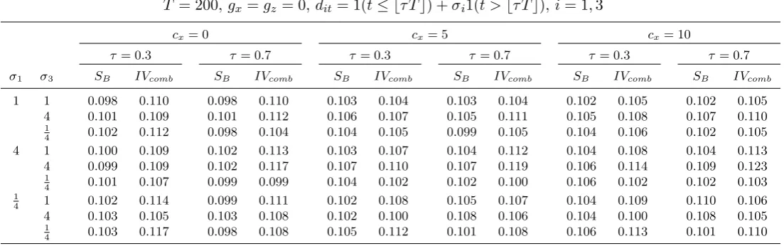
Lastly we examine the impact of unconditional heteroskedasticity in the DGP on the size
ofSBandIVcombwhen the error processes are subject to a single break in volatility.6
Specif-ically, we again simulate the DGP (1)-(3) forT = 200 withgx =gz = 0,et∼IID N(0, I3),
but setting dit = 1(t ≤ bτ Tc) +σi1(t >bτ Tc) for i = 1,3. We set τ = {0.3,0.7} thereby
allowing for two (common) volatility break timings, and σi = {1,4,14} allowing for both
upward and downward volatility shifts (these magnitudes being substantial for illustrative
purposes). We consider cx = {0,5,10} and for simplification abstract from time-varying
correlation between xt and yt by setting h21 =h31=h32 = 0. Table 1 reports the results
for nominal 0.10-level tests (two-sided forIVcomb). It is clear that the size ofSB is very well
controlled across all the patterns of time-varying volatility of xt and yt. The wild
boot-strap aspect of the bootboot-strap methods that we propose therefore works well in achieving
size close to the nominal level even for the large volatility changes that we consider.7 The
IVcomb test also displays a good degree of robustness to heteroskedasticity, although size
can be a little inflated for some settings.
The Supplementary Appendix also contains results for the same settings as above but
with gz = 25 and gz = 50, i.e. power for SB and size for IVcomb, with cz = cx and
additionally allowing for a volatility break in zt via d2t =1(t ≤ bτ Tc) +σ21(t > bτ Tc).
It is clear that the presence of (unconditional) heteroskedasticity can have a substantial
6We do not considert
u andQhere since these procedures are not robust to heteroskedastic errors.
7We also simulated the finite sample size ofS
B under a variety of conditionally heteroskedastic
specifi-cations, including multivariate GARCH and EGARCH, the latter an example of an asymmetric GARCH
influence on the level of power attainable. Other things equal, a volatility increase in
zt (an increase in σ2) leads to higher SB power, with a volatility decrease in zt having
the opposite effect, while volatility changes in yt have the reverse effect, with an increase
(decrease) in σ3 resulting in lower (higher) power for SB. Volatility changes inxt (changes
in σ1) appear to have relatively little effect. A similar pattern of rejection frequencies is
also observed for the sizes of the IVcomb test under heteroskedasticity. In the same cases
where SB power is increased (decreased), so the over-size of IVcomb increases (decreases).
It appears, therefore, that SB has attractive size and power properties in finite samples as
well as in the limit, and it is encouraging to see that for the most part these carry over to
situations where the errors are unconditionally heteroskedastic.
6
An Empirical Application to U.S. Equity Data
To illustrate how our proposed procedure may be used in practice, we reconsider the results
from the empirical analysis investigating the predictability of excess returns using the U.S.
equity data reported in CY. CY consider four different series of stock returns,
dividend-price ratio, and earnings-dividend-price ratio. The first is annual S&P 500 index data over the period
1871–2002. The other three series are annual, quarterly, and monthly NYSE/AMEX
value-weighted index data (1926–2002). Full data descriptions are provided in CY. The data can
be obtained from https://sites.google.com/site/motohiroyogo/home/research/
CY analyse the time series behaviour of these data and test for predictability in excess
returns (relative to an appropriate risk free rate), using as putative predictors for a variety of
sample windows: the dividend-price ratio, denoted d−p; the earnings-price ratio, denoted
e−p; the three-month T-bill rate, denotedr3, and a measure of the long-short yield spread,
denoted y−r1. Details on the construction of these variables can be found in CY; as is
conventional, excess returns and the predictor variables appear in logs. CY argue that all
of these possible predictors display high persistence with, in most cases, the 95% confidence
interval for the largest autoregressive root containing unity. A priori then, bivariate tests of
predictability would seem to be at potential risk from the spurious predictability problem.
Table 2 reports the application of a variety of statistics to the same sets of bivariate