1
Using mixed objects in the training of object-based image classifications
1Hugo Costa, Giles M. Foody, and Doreen S. Boyd 2
School of Geography, University of Nottingham, Nottingham NG7 2RD, UK 3
Abstract 4
Image classification for thematic mapping is a very common application in remote sensing, 5
which is sometimes realized through object-based image analysis. In these analyses, it is common 6
for some of the objects to be mixed in their class composition and thus violate the commonly 7
made assumption of object purity that is implicit in a conventional object-based image analysis. 8
Mixed objects can be a problem throughout a classification analysis, but are particularly 9
challenging in the training stage as they can result in degraded training statistics and act to reduce 10
mapping accuracy. In this paper the potential of using mixed objects in training object-based 11
image classifications is evaluated. Remotely sensed data were submitted to a series of 12
segmentation analyses from which a range of under- to over-segmented outputs were 13
intentionally produced. Training objects were then selected from the segmentation outputs, 14
resulting in training data sets that varied in terms of size (i.e. number of objects) and proportion 15
of mixed objects. These training data sets were then used with an artificial neural network and a 16
generalized linear model, which can accommodate objects of mixed composition, to produce a 17
series of land cover maps. The use of training statistics estimated based on both pure and mixed 18
2
obtained from the use of only pure objects in training. So rather than the mixed objects being a 20
problem, they can be an asset in classification and facilitate land cover mapping from remote 21
sensing. It is, therefore, desirable to recognize the nature of the objects and possibly 22
accommodate mixed objects directly in training. The results obtained here may also have 23
implications for the common practice of seeking an optimal segmentation output, and also act to 24
challenge the widespread view that object-based classification is superior to pixel-based 25
classification. 26
Keywords: OBIA; mixed pixels; under-segmentation; over-segmentation; scale parameter 27
1. Introduction 28
Information on the Earth’s surface such as land cover and related environmental processes is of 29
great importance for a plethora of applications, for example for decision-making on issues related 30
to agriculture and food security (Fritz et al., 2013; Gardi et al., 2015), monitoring the distribution 31
of species (Martin et al., 2013; Tuanmu and Jetz, 2014), and modelling of the Earth’s climate 32
(Luyssaert et al., 2014; Mahmood et al., 2014). For this reason, thematic mapping through a 33
classification analysis is a very common application of remote sensing. Over the years substantial 34
progress has been made in remote sensing-based mapping, and today there are many ways 35
through which a classification analysis can be conducted (Lu and Weng, 2007; Momeni et al., 36
2016). 37
A key decision needed during a classification analysis is on which basic spatial unit to use. 38
3
classification has been common for decades. However, grouping spatially connected pixels into 40
objects by means of an image segmentation analysis, and using the object as the basic spatial unit 41
has become very popular in recent years (Blaschke et al., 2014). The objects obtained from an 42
image segmentation analysis may, in principle, form a more suitable spatial unit than the pixel 43
for land cover mapping as they should relate to natural spatial units (e.g. fields) unlike pixels 44
which are artificial units defined more by the sensing system than the properties of the ground. 45
The use of objects comprising multiple pixels can also aid the calculation of potentially useful 46
discriminatory variables such as descriptors of image texture (Laliberte and Rango, 2009). 47
There are, however, fundamental issues and assumptions of classification that often appear to be 48
ignored or incompletely addressed in object-based image analyses. For example, it is common for 49
the objects produced from the segmentation analysis to be routinely and unquestioningly used as 50
if pure in the classification (e.g. Goodin et al., 2015; Shimabukuro et al., 2015; Uddin et al., 51
2015). However, this is often not the case, mainly for two reasons. First, remotely sensed data 52
inevitably comprise a proportion of mixed pixels whatever the spatial resolution used (Addink et 53
al., 2012; Cracknell, 1998; Fisher, 1997), which cannot be accommodated by traditional image 54
segmentation. For example, Wu (2009) found that 40-50% of the pixels of an urban area 55
represented in multispectral IKONOS data (4 m resolution) were mixed. Second, image 56
segmentation often produces mixed objects as a result of under-segmentation error. This type of 57
error corresponds to situations such as the failure of the image segmentation analysis to define a 58
border splitting two land cover classes, thereby generating a single object containing more than 59
4
Failure to satisfy the assumptions of classification can greatly degrade the quality of the land 61
cover map produced ultimately. In particular, the specific case of under-segmentation error (Gao 62
et al., 2011; Hirata and Takahashi, 2011; Wang et al., 2004) is a problem throughout the 63
classification process as mixed objects can degrade class training statistics, they cannot be 64
appropriately allocated to a single class, and any such allocation must to some extent be 65
erroneous (Heumann, 2011). Action is therefore needed to address the impact of these mixed 66
units. That said, deviation from the assumptions of classification can, however, sometimes be 67
made in each of the main stages of a classification analysis (e.g. Foody, 1999a). Specifically, 68
impure units can be accounted for in training (Eastman and Laney, 2002; Foody, 1997; Hansen, 69
2012; Zhang and Foody, 2001), class allocation (Dronova et al., 2011; Foody, 1996; Wang, 70
1990), and testing a classification (Binaghi et al., 1999; Foody, 1995; Stehman et al., 2007). For 71
example, van de Vlag and Stein (2007) generated objects based on remotely sensed data, 72
classified them using fuzzy decision trees, and produced fuzzy error matrices in accuracy 73
assessment. However, little research has been undertaken on the use of mixed units in training 74
object-based image classifications. 75
Typically, the objects used in training are assumed to be pure (i.e. contain a single class), but a 76
range of options are available if mixed objects are encountered. For example, the analyst could 77
seek to simply ignore the problem, act to exclude the mixed cases, or adopt procedures that can 78
accommodate the mixed nature of the units (Foody, 1999a, 1997). In object-based classification, 79
the presence of mixed objects in training is sometimes addressed beforehand by deliberately 80
5
(Boyden et al., 2013; Cánovas-García and Alonso-Sarría, 2015; Dronova et al., 2012; Van Coillie 82
et al., 2008). However, this approach may be sub-optimal (Dorren, 2003; Gao et al., 2011; Hirata 83
and Takahashi, 2011; Kim et al., 2009; Mishra and Crews, 2014) and is unlikely to remove all 84
impure objects (Zhou et al., 2009; Zhou and Troy, 2008). Another solution sometimes adopted is 85
the exclusion of mixed objects from the production of training statistics (Cai and Liu, 2013; 86
Dean and Smith, 2003; Dronova et al., 2011; Güttler et al., 2016). In this way, the mixed units, 87
which do not satisfy key assumptions of the analysis, are excluded so that the analysis can 88
proceed with suitable data. Excluding mixed objects has, however, the consequence that the size 89
of the training data sets will be reduced, and this could limit the quality of the resulting training 90
statistics. This issue is particularly relevant in object-based classifications as the pool of potential 91
training units is typically relatively small at the outset (Ma et al., 2015). Excluding mixed objects 92
from the pool of selectable objects can exacerbate the challenge of finding a sufficient number of 93
training objects (Mui et al., 2015; Wang et al., 2004). 94
Another issue to take into account while excluding mixed objects is the criteria according to 95
which an object should be considered as mixed. It is unclear whether an object containing a very 96
small fraction of pixels corresponding to a minority class should be excluded from training 97
because there is the chance of those minority pixels having a negligible impact on the training 98
statistics produced. For example, Cai and Liu (2013) excluded from training all objects whose 99
dominant class occupied less than 90% of the objects’ area. The effect of issues such as threshold 100
6
on several factors, such as the remotely sensed data used and the land cover classes mixed 102
(Dronova et al., 2011). 103
The assumptions of a classification also impact on the way training data sets should be used. For 104
example, the training stage of a supervised classification should be designed in relation to the 105
chosen classifier as different algorithms use the data differently. Specifically, with a standard 106
statistical classifier, such as the maximum likelihood classification, it is important that each class 107
is described appropriately which often requires a relatively large and representative training 108
sample (Ediriwickrema and Khorram, 1997; Hagner and Reese, 2007; Paola and Schowengerdt, 109
1995; Richards and Kingsbury, 2014) while the use of a small sample of deliberately selected 110
extreme and atypical samples may be more suited to non-parametric classifiers, such as a 111
multilayer perceptron neural network, support vector machine, and classification tree (Foody, 112
1999b; Foody and Mathur, 2006; Hansen, 2012; Pal and Foody, 2012). Critically, the nature of 113
the data used in training a classification should be acknowledged and addressed. 114
In this paper it is argued that it is not necessary, or even desirable, to exclude mixed objects from 115
training an object-based image classification. In particular, it is possible to turn the apparent 116
problem of mixed units into an asset, as with mixed pixels in per-pixel classification (Foody, 117
1997), recognizing that each individual mixed unit can be a source of training data on more than 118
one class, and that mixed units can be used in training. Here, the potential of using mixed objects 119
in training an object-based image classification is evaluated. A series of image segmentation 120
7
sets that varied in terms of size and proportion of mixed objects. The mixed objects generated at 122
the segmentation stage and encountered at the training stage are included in the set of objects 123
used to estimate training statistics, and the classification outputs produced by two classifiers are 124
evaluated in relation to a conventional analysis using only pure objects. Thus, the work sets out 125
to test the hypothesis that mixed objects may be used in the training of object-based image 126
classifications to increase the accuracy with which land cover may be mapped from remotely 127
sensed data. 128
2. Materials and methods 129
2.1 Study area and data sets
130
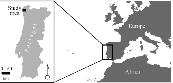
The analyses focused on a test site of approximately 45,000 ha in northern Portugal (Figure 1). 131
The area corresponds to the downstream part of river Lima where the city of Viana do Castelo is 132
settled. A diverse range of land cover types are present in the study area, and five land cover 133
classes were defined: Artificial surfaces, Agricultural areas, Forest and semi-natural areas, Open 134
spaces with little or no vegetation, and Wetlands and water bodies. 135
[image:7.612.76.373.504.648.2]136
8
A Portuguese map, “Carta de Ocupação do Solo” of 2007 (COS2007), was used as reference data 138
set (Figure 2a) in training and testing the object-based classifications. This map was produced by 139
the Portuguese mapping agency (Direção-Geral do Território) through visual interpretation of 140
aerial imagery and use of auxiliarydata such as field work and the national forest inventory. Land 141
cover is represented according to a nomenclature similar to that used in this study in the third of a 142
total of five hierarchical thematic levels used to map land cover with a minimum mapping unit of 143
1 ha (Caetano et al., 2010). As a guide to the thematic accuracy of the map, the overall accuracy 144
is 96.82±1.01% at the 95% confidence level for the thematic detail used in this article, 5 classes, 145
and the producer’s accuracy for each of the classes is >92%. This map provides the most accurate 146
and detailed representation of the land cover that is available for the region and hence is suitable 147
as reference data in the production and assessment of optimal image classifications in this study. 148
9
Figure 2. Data sets used: a) reference land cover map, COS2007, representing Artificial surfaces in red, 150
Agricultural areas in yellow, Forest and semi natural areas in green, Open spaces with little or no 151
vegetation in grey, and Wetlands and water bodies in blue; the square areas outlined in black are the 152
training areas randomly located for the estimation of object-based training statistics. b) LISS-III image 153
collected in Summer of 2006; RGB composition of data acquired in the near infrared, short wave infrared 154
and red bands respectively. 155
Two images acquired during Spring and Summer of 2006 (Figure 2b) by the Linear Imaging Self 156
Scanning Sensor (LISS-III) onboard IRS-P6 (also known as ResourceSat-1) were used. These 157
two images are part of the IMAGE2006 European coverages provided by the European Space 158
Agency (Müller et al., 2009). LISS-III is a multi-spectral camera operating in four spectral bands 159
(green, red, near infrared, and short wave infrared) with a spatial resolution of 23 m in each. The 160
two LISS-III images were orthorectified and resampled to 25 m spatial resolution using an 161
SRTM-based digital elevation model (Müller et al., 2009). The four bands of the two images 162
were stacked and thus formed an eight waveband data set. 163
2.2 Image segmentation
164
The LISS-III data were segmented using the multiresolution algorithm implemented in GeoDMA 165
software (Körting et al., 2013), version 0.2.1, which is based on the popular algorithm of Baatz 166
and Schäpe (2000). This is a region-based algorithm that uses spectral and shape properties of the 167
objects being generated. Colour and shape parameters range within the interval 0-100 and are 168
inversely proportional (i.e. colour=100-shape). In addition, the parameter shape depends on two 169
other parameters, compactness and smoothness, also ranging within the interval 0-100 and 170
10
regard colour, and shape properties. Essentially, the larger the scale parameter value the larger 172
the heterogeneity allowed within objects, thus making larger and fewer objects (Körting et al., 173
2013). 174
The scale, colour, and shape parameter values are the most influential parameters (Luo et al., 175
2015) and were varied to obtain a series of different segmentations. First, five values were 176
defined for the parameter colour, covering the entire range of possible values for this parameter: 177
1, 25, 50, 75, and 99. The importance of the spectral properties of the objects is positively related 178
to the magnitude of the colour parameter. For simplicity, the parameter shape is not discussed 179
hereafter as its value is automatically known for a given value of parameter colour. Then, for 180
each of the five colour parameter values defined, the scale parameter was varied greatly as this is 181
the most influential parameter (Luo et al., 2015). Specifically, eight values were defined from 10 182
to 80 in steps of 10. As a result, 40 segmentation outputs were obtained, ranging from over-183
segmented results mostly composed of small and possibly pure objects to under-segmented 184
results mostly composed of large and possibly mixed objects. For the purposes of this paper an 185
object was taken to be pure if more than 90% of its area was covered with a single class, similar 186
to Cai and Liu (2013). 187
2.3 Training
188
A fraction of the study area was randomly selected for training purposes. Specifically, ten 225 ha 189
square areas were selected randomly to provide training data. As a result, a total of 2250 ha, 190
11
areas were intentionally defined as being small relative to the study area to simulate the limited 192
availability of reference data that are typical of real-world applications. The objects of each of the 193
segmentation outputs that intersected the training areas were selected for the production of 194
training statistics. The objects generated via image segmentation are commonly used for 195
estimating training statistics (e.g. Goodin et al., 2015). Thus, while the same geographical area 196
was used in training each classification the set of objects used varied between the segmentation 197
outputs. As a result, the training statistics varied between segmentation settings. In all cases, 198
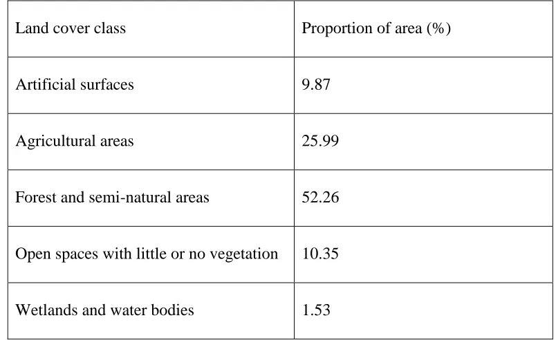
however, the representation of the land cover classes was constant and proportional to their 199
[image:11.612.61.463.397.643.2]abundance (Table 1) as the training areas defined were constant and randomly located. 200
Table 1. Proportion of area of the land cover classes mapped in the reference COS2007 land cover map 201
in the training areas defined. The relative proportion of the classes is common to all training statistics 202
estimated from the segmentation settings used. 203
Land cover class Proportion of area (%)
Artificial surfaces 9.87
Agricultural areas 25.99
Forest and semi-natural areas 52.26
Open spaces with little or no vegetation 10.35
Wetlands and water bodies 1.53
12
The mean and standard deviation of the digital numbers of each object in the eight LISS-III 205
spectral bands were used as training statistics, resulting in a total of 16 discriminating variables. 206
The training objects were assigned reference class labels extracted from the COS2007 land cover 207
map. The proportion of the area that each class occupied in a training object was estimated, 208
ranging from 0.0 if the class was absent to the maximum value of 1.0 if the object was pure, with 209
intermediate values for at least two classes if the object was of mixed class composition. 210
The remotely sensed data were classified using each of the segmentation outputs produced. Two 211
scenarios were followed. First, following the traditional procedure of using only pure objects at 212
the training stage. Specifically, each object intercepting the training areas was taken as pure and 213
hence allowed to be a training object only for the class with which had the maximum 214
membership based on the proportion of class area, which had to be superior to 90% (otherwise 215
they were excluded from training). Second, all of the training objects, even if some were mixed, 216
were used. The fractional coverage of the classes found in the objects was used as a measure of 217
class membership, and training objects were allowed multiple and partial membership. 218
Because mixed objects were not excluded from training in the mixed training strategy, the size of 219
the mixed training data sets was typically larger than when only pure objects were used. Since the 220
size of the training set may impact the classification accuracy (Ma et al., 2015; Millard and 221
Richardson, 2015) a series of analyses in which training set size was constant was also 222
undertaken. For this additional analyses, reduced versions of the mixed training data sets were 223
13
data sets. The reduction of the size of the mixed training data sets was achieved by excluding 225
randomly selected objects. Since the mixed training data sets may comprise both pure and mixed 226
objects, this approach means that all objects, pure and mixed, had the same probability of being 227
excluded. This allowed the size of the training data sets to be reduced without changing 228
substantially the inherent ratio of pure to mixed objects. As the random exclusion of objects can 229
result in numerous and different training data sets each of which with a potential different impact 230
on the results, three reduced mixed training data sets were produced from each mixed training 231
data set. 232
A series of classifications of the remotely sensed data using all 40 segmentation outputs was 233
produced. With each segmentation output, classifications were produced that were trained using 234
(i) pure training data sets, (ii) mixed training data sets, and (iii) the reduced (to same size as pure) 235
training data sets. 236
2.4 Classification
237
In all analyses, multinomial regression models fitted by means of an artificial neural network 238
with no hidden layer (Venables and Ripley, 2002) and a generalized linear model via penalized 239
maximum likelihood (Friedman et al., 2010) were used for classification. These classifiers are 240
available in the R programing language (R Core Team, 2016) from the packages ‘nnet’ and 241
‘glmnet’ respectively. Both classifiers allow fractional composition of the objects to be used in 242
14
The output of the classifiers is soft, indicating the probability of an object belonging to each class 244
(Friedman et al., 2010; Venables and Ripley, 2002). However, traditional hard land cover maps 245
were estimated by allocating each object the label of the class with which it had the greatest 246
probability of membership. Although it may be beneficial to address the potential mixed nature 247
of the objects at the class allocation stage, hard classification was adopted to confine the focus of 248
the paper to the training stage. Each segmented image was thus used to produce hard land cover 249
maps based on different training strategies: pure, mixed, and reduced mixed. 250
2.5 Accuracy assessment
251
The thematic accuracy of each classification produced was assessed. Confusion matrices 252
comparing the land cover maps produced and the reference COS2007 land cover map were 253
constructed through an operation of spatial intersection of the two data layers. Thus, instead of 254
using a sample to estimate classification accuracy, the entire study area was used to assess the 255
accuracy with which each of the 40 segmentation outputs produced was classified. Note, 256
however, that the area associated with training (Figure 2a) was not used for accuracy assessment 257
because that would artificially increase classification accuracy. Classification accuracy was 258
expressed in terms of proportion of area correctly classified. Because the entire study area was 259
used to estimate proportions of area correctly and incorrectly classified, the issues of selecting 260
either pixels or objects as sampling units and producing estimates of accuracy which holds 261
15
The accuracy of the 40 segmentation outputs generated was also assessed to provide a measure of 263
under- and over-segmentation error, which is useful for analysis of the results. The method 264
developed by Möller et al. (2013) and slightly refined by Costa et al. (2015) was used. This 265
method belongs to a popular family of methods widely known as empirical discrepancy or 266
supervised methods (Clinton et al., 2010; Zhang, 1996), and essentially compares the image 267
segmentation output under evaluation to a reference data set (e.g. land cover map) to measure the 268
geometric match between the objects that form them. Möller et al.’s (2013) method includes 269
typical area-based and position-based metrics such as the ratio of overlapping area among 270
generated and reference objects and the distance between the objects’ centroid (Clinton et al., 271
2010; Whiteside et al., 2014) to detected and measure under- and over-segmentation error 272
separately. The metrics are the basis for finding an optimal segmentation output that offsets the 273
two types of error while informing on which type predominates when unbalanced, which is 274
useful for this study. A summary of the segmentation accuracy is provided by metric Mg which 275
measures the strength and type of segmentation error. Negative Mg values indicate that under-276
segmentation error dominates while positive Mg values represent the opposite case in which 277
over-segmentation error dominates. Therefore, Mg~0 is considered indicative of optimal 278
segmentation accuracy as both types of error are balanced (Möller et al., 2013). The reference 279
data set used was the set of polygons of the COS2007 land cover map over the training areas 280
defined. Thus, it was possible to determine whether the training data sets used were over-281
16 3. Results
283
The 40 segmentation outputs generated varied greatly in nature from over- to under-segmented, 284
as expected, and two examples are shown in Figure 3 to highlight the different sets of objects 285
obtained. The geometric accuracy of the objects that intersected the training areas, and hence 286
used for training, was assessed, and the results are presented in Figure 4. Small values of the 287
parameter scale produced over-segmented training objects (Mg>0) while large scale values 288
yielded under-segmented outputs (Mg<0). For intermediate scale values, the type and magnitude 289
of segmentation error became less evident. According to the Costa et al.’s (2015) adaptation of 290
Möller et al.’s (2013) method, the scale value of 10, 30, 40, 50, and 70 were close to being 291
optimal when the parameter colour was set at 1, 25, 50, 75, and 99, respectively, as Mg∼0. 292
293
Figure 3. Segmentation results: a) Segmentation output produced with colour=75 and scale=10. b) 294
17 296
Figure 4. Segmentation accuracy based on Costa et al.’s (2015) adaptation of Möller et al.’s (2013) 297
method. Dotted horizontal line corresponds to optimal accuracy. 298
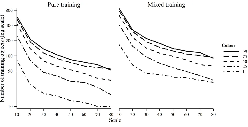
The range of segmentation outputs generated resulted in training data sets of varying sizes 299
(Figure 5). The number of training objects was large when over-segmentation was large (i.e. 300
small values of parameter scale), and decreased as the level of under-segmentation increased. For 301
example, when the parameter scale was set at 10 and 80, the training data sets generated 302
comprised >430 and <100 training objects respectively. For a same value of parameter scale, 303
larger training data sets were obtained when parameter colour was large. In all cases, some 304
objects were mixed and hence the number of pure objects generated by a segmentation analysis 305
was always less than the total number of objects generated. As such more objects were available 306
for training when mixed rather than only pure objects were allowed. Specifically, 30-70% of the 307
total number of the training objects was excluded when only pure objects were permitted in 308
training. For example, the apparently near optimal segmentation output generated using 309
colour=50 and scale=40 comprised 113 objects of which only 62 were pure (Figure 5). Thus, 51 310
18
objects were allowed in training using an apparently near optimal segmentation. Mixed objects 312
should, therefore, be expected to occur and even be common in object-based analyses. 313
[image:18.612.76.507.146.367.2]314
Figure 5. Size of training data sets. 315
The nature of the training data sets had a considerable impact on classification accuracy 316
regardless of the classifier used. In general, the generalized linear model enabled classification to 317
reach larger accuracy than the artificial neural network due to the regularization procedure of the 318
former, but the results are consistent between them while excluding or allowing mixed objects in 319
training. Critically, the magnitude of classification accuracy was consistently smaller for the 320
classifications that excluded mixed objects in training relative to that which allowed mixed 321
objects (Figure 6). For example, using the artificial neural network and segmentation output 322
colour=50 and scale=40, the classification accuracy was 50.4 and 69.0% when the pure and 323
19
differences observed in terms of classification accuracy were so substantial that the smallest 325
accuracy achieved with the use of the mixed training data sets (57.7%; point C in Figure 6b, 326
using 33 training objects) was larger than the largest accuracy achieved with the use of only pure 327
training data (54.7%; point D in Figure 6i, using 540 training objects) if the results obtained with 328
colour=1 (Figure 6b and Figure 6f) are ignored. The minimum value of parameter colour was 329
associated with somewhat atypical results. For example, the segmentation settings defined by 330
colour=1 and scale=80 are associated with an increase in classification accuracy when trained 331
with only pure objects, but the quality of the land cover maps is very small. Specifically, virtually 332
the entire study area was classified as Forest and semi-natural areas class, and hence the 333
classification accuracy tends to converge with the proportion of the study area covered by that 334
class (~50%). The results obtained using colour=1 were caused mainly by the extremely small 335
consideration of spectral information while generating the objects, and thereby relatively large 336
values for the parameter colour are commonly used. The results obtained with this particular 337
value of parameter colour are not referred or discussed hereafter for simplicity. 338
The reduced mixed training data sets also afforded larger classification accuracy than the pure 339
training data sets. For example, the reduced mixed training data sets used to classify the 340
segmentation output produced using colour=50 and scale=40 were enough for the accuracy of the 341
artificial neural network to reach 61.6, 63.8, and 65.8% (points E in Figure 6c, Figure 7c,d), 342
substantially more than with the use of pure training data (50.4%; point A in Figure 6c). There 343
are a few cases in which the reduced mixed training data sets produced slightly larger 344
20
and scale were large and small respectively (Figure 6e and Figure 5j). Thus, the difference in the 346
accuracy achieved with the use of pure and mixed training sets is not simply an issue of training 347
set size; mixed objects appear useful to produce valuable discriminatory information. The ability 348
to increase classification accuracy through the use of mixed training objects should help the 349
production of land cover maps that meet user needs and exceed appropriate target accuracy 350
values (Foody, 2008). The key issue in relation to the hypothesis being tested in this article, 351
however, is that the use of mixed objects can substantially increase classification accuracy 352
relative to that achieved when only pure training objects are used. The difference in accuracy 353
arising from the use of mixed and pure training sets varied with the specific parameter settings of 354
the classifications, but was typically large. Specifically, difference in accuracy between 355
classifications trained using pure and mixed training sets was up to 36% but typically in the order 356
21 358
Figure 6. Classification accuracy as a function of the parameter scale with parameter colour set at 1, 25, 359
50, 75, and 99. The results obtained using the three reduced versions of the mixed training data sets are 360
identified as #1, #2, and #3. Panel a) to e) and f) to j) refer to the artificial neural network and 361
22 363
Figure 7. Land cover maps obtained using the segmentation output produced with colour=50 and 364
scale=40, the artificial neural network, and different training strategies. a) Pure training (accuracy: 365
50.4%). b) Mixed training (accuracy: 69.0%). c) Mixed training with reduced samples #1 (accuracy: 366
61.5%). d) Mixed training with reduced samples #3 (accuracy: 65.8%). Colour legend as in Figure 2. 367
Beyond the evident difference between the classifications generated with pure and mixed, even if 368
reduced, training data, there is a clear positive trend in classification accuracy with over-369
segmentation. The largest overall accuracies were reached using scale=10 regardless of the 370
colour parameter values defined (25, 50, 75, or 99) and training strategy used (pure or mixed). 371
However, there were differences in the way classification accuracy varied as a function of the 372
23
when the entire mixed training data sets were used (smooth decreasing red lines in Figure 6); 374
classification accuracy decreased variably when the reduced mixed training data sets were used 375
(fluctuating decreasing grey lines in Figure 6), which is likely due to the random exclusion of 376
specific training objects – objects with more or less impact on the training statistics could be 377
excluded; finally, classification accuracy also tended to decrease as a function of the parameter 378
scale when the pure training data sets were used, but marked variations are visible in Figure 6 379
(fluctuating blue lines). Overall accuracy sometimes peaked locally around the regions indicated 380
as being close to balanced segmentation errors (Mg∼0), for example when the colour parameter 381
was set at 50 and 75 and the artificial neural network was used (point A in Figure 6c and point F 382
in Figure 6d). The local peaks around the regions indicated as being close to balanced 383
segmentation errors agree with numerous studies reporting that segmentation results neither over- 384
nor under-segmented are associated with land cover maps of larger thematic accuracy which have 385
been produced via an image classification analysis trained with pure data (Dorren, 2003; Gao et 386
al., 2011; Hirata and Takahashi, 2011; Kim et al., 2009; Kim and Warner, 2011; Mishra and 387
Crews, 2014). 388
4. Discussion 389
Object-based classification of LISS-III data benefited from allowing training data sets to include 390
mixed objects. An important advantage of mixed training is the opportunity to use relatively 391
large training data sets since there is no need to exclude mixed objects. Furthermore, mixed 392
objects allow efficiency as they give information on more than one class. It is well-known that 393
24
Millard and Richardson, 2015). However, the size of the training data sets is not the only factor 395
explaining the results obtained. When the parameter scale was set at small values, the pure 396
training data sets were large, but the classification accuracy continued to be relatively small. On 397
the contrary, mixed training afforded larger classification accuracy than pure training, even when 398
the mixed training data sets were small. Indeed, the results obtained from the reduced mixed 399
training data sets are closer to those obtained from the full mixed rather than the pure training 400
data sets. Note that the difference in classification accuracy achieved with full and reduced mixed 401
training data sets shrank with an increase in over-segmentation (Figure 6). This suggests that the 402
size of the training data sets produced from extremely over-segmented outputs is not entirely 403
needed, that is a smaller number of training objects may be sufficient to produce similar 404
classification results as long as mixed objects are allowed in training. 405
Mixed objects provide useful discriminatory information, and this may be the main advantage of 406
allowing mixed objects in training. Specifically, a representative sample of the objects generated 407
is used, which includes objects of mixed in addition to pure class composition. Thus, classifiers 408
can learn that the spectral properties of the objects may steam from the spectral signature of 409
thematic classes as well as their mixture. Mixed units must convey information on more than one 410
class and also will, in feature space, tend to lie between the classes involved. As a result of the 411
latter the mixed units may be expected to lie close to the classification hyperplane that separates 412
the classes. Mixed units, therefore, may have the potential to aid class separation, the central aim 413
of a classification analysis. This potential can be exploited when the classifier can directly 414
25
statistics, directly (Foody, 1999b; Foody and Mathur, 2006). Focus on separability rather than 416
description of classes has been focus of innovative learning methods in recent years, such as 417
active learning with mixed spectral responses (Samat et al., 2016). This may be especially 418
relevant for classification as mixed objects may be common in an image segmentation output. 419
The use of mixed units is not without challenges. For example, due to intra-class spectral 420
variation it is possible for units of slightly different thematic composition to have the exact same 421
spectral response. However, the general trend is for mixed units to lie between the relevant 422
classes in feature space. The exact position in feature space is a function of the mixing. A unit 423
dominated by one class might be expected to lie relatively close to that class and still be distant 424
from the other(s) involved while one of more equal mixing lies more centrally between the 425
classes; exact details will depend on the specific classes and details (Foody, 2000; Hill et al., 426
2007; Lee and Lathrop, 2006; Zhu et al., 2013). Another difference between the pure and mixed 427
training strategies relates to the fluctuating classification accuracy observed across the range of 428
segmentation levels used. The accuracy of the classifications that used only pure training data 429
was highly variable as a function of the parameter scale. These results were possibly caused by 430
the imbalanced number of training objects per class (Table 1) and the relatively small size of the 431
pure training data sets (Ma et al., 2015). Imbalanced training sets and the limited spectral 432
resolution of the data used may have set limits to the achievable accuracy and larger accuracy 433
could potentially be achieved with a larger, more balanced, training set and hyperspectral data 434
26
benefited classification accuracy irrespective of the training strategy followed because the 436
spectral content of the remotely sensed data gained importance for the generation of the objects. 437
The fluctuating classification accuracy associated with pure training sometimes showed a peak 438
with segmentation settings which were near to optimal (e.g. point A in Figure 6c and point F in 439
Figure 6d). This may suggest that larger accuracy of the image segmentation analysis offers 440
larger classification accuracy and justifies the common practice for searching for optimal image 441
segmentation results (Dorren, 2003; Gao et al., 2011; Hirata and Takahashi, 2011; Kim et al., 442
2009; Kim and Warner, 2011; Mishra and Crews, 2014). Indeed, since image segmentation and 443
object-based classification have become popular methods for land cover mapping, the body of 444
literature dedicated to methods for parameterization and accuracy assessment of image 445
segmentation has grown (Clinton et al., 2010; Whiteside et al., 2014; Yang et al., 2015). 446
Typically, these methods are focused on finding a segmentation result considered as being 447
optimal in the sense that over- and under-segmentation error are minimal and balanced. 448
However, a comprehensive analysis of the results shows that over-segmentation is associated 449
with larger classification accuracy, and thus the assessment of segmentation accuracy is not 450
necessarily informative for the prediction of an accuracy object-based classification (Figure 4 and 451
Figure 6; Li et al., 2016; Ma et al., 2015). A number of studies (Belgiu and Drǎguţ, 2014; 452
Räsänen et al., 2013; Verbeeck et al., 2012) have observed that classification accuracy and 453
segmentation accuracy, the latter at least as defined by empirical discrepancy methods, may not 454
27
It was notable that the results showed a positive trend of classification accuracy with over-456
segmentation. In the situation of over-segmentation the size and spectral content of the objects 457
generated become close to those of the pixels, and thus the results suggest that classification 458
accuracy might possibly reach a maximum if per-pixel or near to per-pixel (Dronova et al., 2012; 459
Ju et al., 2005) classification had been undertaken. Comparing object-based and per-pixel image 460
classification has received much attention, and some publications have reported similar or larger 461
accuracy of per-pixel classification as compared to object-based classification (Cai and Liu, 462
2013; Goodin et al., 2015; Robertson and King, 2011). However, the majority of the literature 463
actually appears to hold the contrary view, that is that object-based classification achieves larger 464
accuracy than per-pixel (Estoque et al., 2015; Goodin et al., 2015; Memarian et al., 2013; 465
Whiteside et al., 2011). Apparently, the view that object-based classification is superior to per-466
pixel classification has become widespread and commonly unquestionable. The results presented 467
above emphasize the need for more research in this respect. For example, typical comparisons 468
between object-based and per-pixel classifications have relied on pure training, while the use of 469
mixed training, which is also beneficial for per-pixel classification (Eastman and Laney, 2002; 470
Foody, 1997; Hansen, 2012; Zhang and Foody, 2001), should be considered in comparative 471
studies. Furthermore, it should be taken into account that the suitability of per-pixel and object-472
based classifications may depend on scale issues related to the land cover patterns on the ground, 473
and the spatial resolution of the remotely sensed data and classification nomenclature used. For 474
28
classes mapped (Castilla et al., 2014; Kim and Warner, 2011; Laliberte and Rango, 2009) not 476
least because the definition of categorical classes is a scale dependent issue (Ju et al., 2005). 477
Finally, this study used an artificial neural network and generalized linear model able to 478
accommodate mixed objects which is a fundamental aspect to take into account if training using 479
impure units is to be undertaken. Alternative parametric classifiers, such as the maximum 480
likelihood classification provided in commonly used software packages, may be less appropriate 481
as relatively large and representative samples formed by pure training units are needed to 482
describe the classes; unless the training statistics are rectified. For example, the component parts 483
of a mixed object can be unmixed and used to estimate the signal of the object as it would be if 484
pure (Foody and Arora, 1996). The use of mixed objects for training a classification is, therefore, 485
possible for a range of classifiers and may facilitate land cover mapping from remote sensing. 486
The mixed nature of the spatial units used may also be addressed at the class allocation stage as 487
partial and multi class membership are estimated, which can then be assessed based, for example, 488
on the fuzzy confusion matrix (Binaghi et al., 1999; Stehman et al., 2007). This paper focused on 489
the training stage, but a fully fuzzy classification approach may be implemented for thematic 490
mapping (Foody, 1997; Zhang and Foody, 2001). 491
5. Conclusions 492
An implicit assumption made typically in object-based image classification is that the objects are 493
pure. This is often not the case, and in this paper it was shown that mixed objects can be 494
29
common practice, it may be, therefore, not necessary to remove mixed objects from the training 496
stage of a supervised image classification. Rather, an analysis of the effects of allowing mixed 497
objects in training should be considered, which also affords an increase in the size of the training 498
data set, and may contribute to an increase in classification accuracy. For example, by using 499
mixed objects in this study often the overall accuracy increased by around 25% relative to that 500
achieved using pure objects only. Furthermore, the results suggest that it may not be necessary to 501
follow common practice and seek an optimal segmentation output. Specifically, deliberate over-502
segmentation may be a suitable strategy for generating objects for optimal training. 503
Acknowledgements 504
The authors are grateful to Markus Möller from the University of Halle (Saale) for providing R 505
code, the LISS-III data used was provided by the European Space Agency, and the research was 506
supported by the PhD Studentship SFRH/BD/77031/2011 from the “Fundação para a Ciência e 507
Tecnologia” (FCT), funded by the “Programa Operacional Potencial Humano” (POPH) and the 508
European Social Fund. The quality of the original manuscript was improved based on valuable 509
suggestions of anonymous reviewers and the Associate Editor. 510
References 511
Addink, E.A., Van Coillie, F.M.B., De Jong, S.M., 2012. Introduction to the GEOBIA 2010 512
special issue: From pixels to geographic objects in remote sensing image analysis. Int. J. 513
Appl. Earth Obs. Geoinf. 15, 1–6. doi:10.1016/j.jag.2011.12.001 514
Baatz, M., Schäpe, A., 2000. Multiresolution Segmentation: an optimization approach for high 515
quality multi-scale image segmentation, in: Strobl, J., Blaschke, T., Griesebner, G. (Eds.), 516
30
Salzburg 2000. Herbert Wichmann Verlag, Heidelberg, pp. 12–23. 518
Belgiu, M., Drǎguţ, L., 2014. Comparing supervised and unsupervised multiresolution 519
segmentation approaches for extracting buildings from very high resolution imagery. ISPRS 520
J. Photogramm. Remote Sens. 96, 67–75. doi:10.1016/j.isprsjprs.2014.07.002 521
Binaghi, E., Brivio, P.A., Ghezzi, P., Rampini, A., 1999. A fuzzy set-based accuracy assessment 522
of soft classification. Pattern Recognit. Lett. 20, 935–948. doi:10.1016/S0167-523
8655(99)00061-6 524
Blaschke, T., Hay, G.J., Kelly, M., Lang, S., Hofmann, P., Addink, E.A., Queiroz Feitosa, R., 525
van der Meer, F., van der Werff, H., van Coillie, F., Tiede, D., 2014. Geographic Object-526
Based Image Analysis – Towards a new paradigm. ISPRS J. Photogramm. Remote Sens. 87, 527
180–191. doi:10.1016/j.isprsjprs.2013.09.014 528
Boyden, J., Joyce, K.E., Boggs, G., Wurm, P., 2013. Object-based mapping of native vegetation 529
and para grass (Urochloa mutica) on a monsoonal wetland of Kakadu NP using a Landsat 5 530
TM Dry-season time series. J. Spat. Sci. 58, 53–77. doi:10.1080/14498596.2012.759086 531
Caetano, M., Nunes, A., Dinis, J., Pereira, M. d. C., Marrecas, P., Nunes, V., 2010. Carta de uso 532
e ocupação do solo de Portugal Continental para 2007: Memória descritiva. Instituto 533
Geográfico Português, Lisbon. 534
Cai, S., Liu, D., 2013. A comparison of object-based and contextual pixel-based classifications 535
using high and medium spatial resolution images. Remote Sens. Lett. 4, 998–1007. 536
doi:10.1080/2150704X.2013.828180 537
Cánovas-García, F., Alonso-Sarría, F., 2015. A local approach to optimize the scale parameter in 538
multiresolution segmentation for multispectral imagery. Geocarto Int. 30, 937–961. 539
doi:10.1080/10106049.2015.1004131 540
Carrão, H., Goncalves, P., Caetano, M., 2008. Contribution of multispectral and multitemporal 541
information from MODIS images to land cover classification. Remote Sens. Environ. 112, 542
986–997. doi:10.1016/j.rse.2007.07.002 543
Castilla, G., Hernando, A., Zhang, C., McDermid, G.J., 2014. The impact of object size on the 544
thematic accuracy of landcover maps. Int. J. Remote Sens. 35, 1029–1037. 545
doi:10.1080/01431161.2013.875630 546
Clinton, N., Holt, A., Scarborough, J., Yan, L., Gong, P., 2010. Accuracy assessment measures 547
for object-based image segmentation goodness. Photogramm. Eng. Remote Sensing 76, 548
289–299. 549
31
sensitivity into image segmentation quality assessment. Photogramm. Eng. Remote Sensing 551
81, 451–459. doi:10.14358/PERS.81.6.451 552
Cracknell, A.P., 1998. Synergy in remote sensing-what’s in a pixel? Int. J. Remote Sens. 19, 553
2025–2047. 554
Dean, A.M., Smith, G.M., 2003. An evaluation of per-parcel land cover mapping using 555
maximum likelihood class probabilities. Int. J. Remote Sens. 24, 2905–2920. 556
doi:10.1080/01431160210155910 557
Dorren, L., 2003. Improved Landsat-based forest mapping in steep mountainous terrain using 558
object-based classification. For. Ecol. Manage. 183, 31–46. doi:10.1016/S0378-559
1127(03)00113-0 560
Dronova, I., Gong, P., Clinton, N.E., Wang, L., Fu, W., Qi, S., Liu, Y., 2012. Landscape analysis 561
of wetland plant functional types: The effects of image segmentation scale, vegetation 562
classes and classification methods. Remote Sens. Environ. 127, 357–369. 563
doi:10.1016/j.rse.2012.09.018 564
Dronova, I., Gong, P., Wang, L., 2011. Object-based analysis and change detection of major 565
wetland cover types and their classification uncertainty during the low water period at 566
Poyang Lake, China. Remote Sens. Environ. 115, 3220–3236. 567
doi:10.1016/j.rse.2011.07.006 568
Eastman, J.R., Laney, R.M., 2002. Bayesian soft classification for sub-pixel analysis: a critical 569
evaluation. Photogramm. Eng. Remote Sens. 68, 1149–1154. 570
Ediriwickrema, J., Khorram, S., 1997. Hierarchical maximum-likelihood classification for 571
improved accuracies. IEEE Trans. Geosci. Remote Sens. 35, 810–816. 572
doi:10.1109/36.602523 573
Estoque, R.C., Murayama, Y., Akiyama, C.M., 2015. Pixel-based and object-based 574
classifications using high- and medium-spatial-resolution imageries in the urban and 575
suburban landscapes. Geocarto Int. 30, 1113–1129. doi:10.1080/10106049.2015.1027291 576
Fisher, P., 1997. The pixel: A snare and a delusion. Int. J. Remote Sens. 18, 679–685. 577
doi:10.1080/014311697219015 578
Foody, G.M., 2008. Harshness in image classification accuracy assessment. Int. J. Remote Sens. 579
29, 3137–3158. doi:10.1080/01431160701442120 580
Foody, G.M., 2000. Estimation of sub-pixel land cover composition in the presence of untrained 581
32
Foody, G.M., 1999a. The continuum of classification fuzziness in thematic mapping. 583
Photogramm. Eng. Remote Sensing 65, 443–451. 584
Foody, G.M., 1999b. The significance of border training patterns in classification by a 585
feedforward neural network using back propagation learning. Int. J. Remote Sens. 20, 3549– 586
3562. doi:10.1080/014311699211192 587
Foody, G.M., 1997. Fully fuzzy supervised classification of land cover from remotely sensed 588
imagery with an artificial neural network. Neural Comput. Appl. 5, 238–247. 589
doi:10.1007/BF01424229 590
Foody, G.M., 1996. Approaches for the production and evaluation of fuzzy land cover 591
classifications from remotely-sensed data. Int. J. Remote Sens. 17, 1317–1340. 592
doi:10.1080/01431169608948706 593
Foody, G.M., 1995. Cross-entropy for the evaluation of the accuracy of a fuzzy land cover 594
classification with fuzzy ground data. ISPRS J. Photogramm. Remote Sens. 50, 2–12. 595
doi:10.1016/0924-2716(95)90116-V 596
Foody, G.M., Arora, M.K., 1996. Incorporating mixed pixels in the training, allocation and 597
testing stages of supervised classifications. Pattern Recognit. Lett. 17, 1389–1398. 598
doi:10.1016/S0167-8655(96)00095-5 599
Foody, G.M., Mathur, A., 2006. The use of small training sets containing mixed pixels for 600
accurate hard image classification: Training on mixed spectral responses for classification 601
by a SVM. Remote Sens. Environ. 103, 179–189. doi:10.1016/j.rse.2006.04.001 602
Friedman, J., Hastie, T., Tibshirani, R., 2010. Regularization Paths for Generalized Linear 603
Models via Coordinate Descent. J. Stat. Softw. 33, 1–22. doi:10.1359/JBMR.0301229 604
Fritz, S., See, L., You, L., Justice, C., Becker-Reshef, I., Bydekerke, L., Cumani, R., Defourny, 605
P., Erb, K., Foley, J., Gilliams, S., Gong, P., Hansen, M., Hertel, T., Herold, M., Herrero, 606
M., Kayitakire, F., Latham, J., Leo, O., McCallum, I., Obersteiner, M., Ramankutty, N., 607
Rocha, J., Tang, H., Thornton, P., Vancutsem, C., van der Velde, M., Wood, S., Woodcock, 608
C., 2013. The need for improved maps of global cropland. Eos, Trans. Am. Geophys. Union 609
94, 31–32. doi:10.1002/2013EO030006 610
Gao, Y., Mas, J.F., Kerle, N., Pacheco, J.A.N., 2011. Optimal region growing segmentation and 611
its effect on classification accuracy. Int. J. Remote Sens. 32, 3747–3763. 612
doi:10.1080/01431161003777189 613
Gardi, C., Panagos, P., Van Liedekerke, M., Bosco, C., De Brogniez, D., 2015. Land take and 614
food security: assessment of land take on the agricultural production in Europe. J. Environ. 615
33
Goodin, D.G., Anibas, K.L., Bezymennyi, M., 2015. Mapping land cover and land use from 617
object-based classification: An example from a complex agricultural landscape. Int. J. 618
Remote Sens. 36, 4702–4723. doi:10.1080/01431161.2015.1088674 619
Güttler, F.N., Ienco, D., Poncelet, P., Teisseire, M., 2016. Combining transductive and active 620
learning to improve object-based classification of remote sensing images. Remote Sens. 621
Lett. 7, 358–367. doi:10.1080/2150704X.2016.1142678 622
Hagner, O., Reese, H., 2007. A method for calibrated maximum likelihood classification of 623
forest types. Remote Sens. Environ. 110, 438–444. doi:10.1016/j.rse.2006.08.017 624
Hansen, M., 2012. Classification trees and mixed pixel training data, in: Remote Sensing of Land 625
Use and Land Cover, Remote Sensing Applications Series. CRC Press, pp. 127–136. 626
doi:doi:10.1201/b11964-12 627
Heumann, B.W., 2011. An Object-Based Classification of Mangroves Using a Hybrid Decision 628
Tree—Support Vector Machine Approach. Remote Sens. 3, 2440–2460. 629
doi:10.3390/rs3112440 630
Hill, R., Granica, K., Smith, G.M., Schardt, M., 2007. Representation of an alpine treeline 631
ecotone in SPOT 5 HRG data. Remote Sens. Environ. 110, 458–467. 632
doi:10.1016/j.rse.2006.11.031 633
Hirata, Y., Takahashi, T., 2011. Image segmentation and classification of Landsat Thematic 634
Mapper data using a sampling approach for forest cover assessment. Can. J. For. Res. 41, 635
35–43. doi:10.1139/X10-130 636
Ju, J., Gopal, S., Kolaczyk, E.D., 2005. On the choice of spatial and categorical scale in remote 637
sensing land cover classification. Remote Sens. Environ. 96, 62–77. 638
doi:10.1016/j.rse.2005.01.016 639
Kim, M., Madden, M., Warner, T.A., 2009. Forest type mapping using object-specific texture 640
measures from multispectral Ikonos Imagery: Segmentation quality and image classification 641
issues. Photogramm. Eng. Remote Sensing 75, 819–829. 642
Kim, M., Warner, T., 2011. Multi-scale GEOBIA with very high spatial resolution digital aerial 643
imagery: scale, texture and image objects. Int. J. Remote Sens. 32, 2825–2850. 644
doi:10.1080/01431161003745608 645
Körting, T.S., Garcia Fonseca, L.M., Câmara, G., 2013. GeoDMA—Geographic Data Mining 646
Analyst. Comput. Geosci. 57, 133–145. doi:10.1016/j.cageo.2013.02.007 647
Laliberte, A.S., Rango, A., 2009. Texture and scale in object-based analysis of subdecimeter 648
34 1–10. doi:10.1109/TGRS.2008.2009355 650
Lee, S., Lathrop, R.G., 2006. Subpixel analysis of landsat ETM + using Self-Organizing Map 651
(SOM) neural networks for urban land cover characterization. IEEE Trans. Geosci. Remote 652
Sens. 44, 1642–1654. doi:10.1109/TGRS.2006.869984 653
Li, M., Ma, L., Blaschke, T., Cheng, L., Tiede, D., 2016. A systematic comparison of different 654
object-based classification techniques using high spatial resolution imagery in agricultural 655
environments. Int. J. Appl. Earth Obs. Geoinf. 49, 87–98. doi:10.1016/j.jag.2016.01.011 656
Lu, D., Weng, Q., 2007. A survey of image classification methods and techniques for improving 657
classification performance. Int. J. Remote Sens. 28, 823–870. 658
doi:10.1080/01431160600746456 659
Luo, H., Wang, L., Shao, Z., Li, D., 2015. Development of a multi-scale object-based shadow 660
detection method for high spatial resolution image. Remote Sens. Lett. 6, 59–68. 661
doi:10.1080/2150704X.2014.1001079 662
Luyssaert, S., Jammet, M., Stoy, P.C., Estel, S., Pongratz, J., Ceschia, E., Churkina, G., Don, A., 663
Erb, K., Ferlicoq, M., Gielen, B., Grünwald, T., Houghton, R.A., Klumpp, K., Knohl, A., 664
Kolb, T., Kuemmerle, T., Laurila, T., Lohila, A., Loustau, D., McGrath, M.J., Meyfroidt, P., 665
Moors, E.J., Naudts, K., Novick, K., Otto, J., Pilegaard, K., Pio, C.A., Rambal, S., 666
Rebmann, C., Ryder, J., Suyker, A.E., Varlagin, A., Wattenbach, M., Dolman, A.J., 2014. 667
Land management and land-cover change have impacts of similar magnitude on 668
surface temperature. Nat. Clim. Chang. 4, 389–393. doi:10.1038/nclimate2196 669
Ma, L., Cheng, L., Li, M., Liu, Y., Ma, X., 2015. Training set size, scale, and features in 670
Geographic Object-Based Image Analysis of very high resolution unmanned aerial vehicle 671
imagery. ISPRS J. Photogramm. Remote Sens. 102, 14–27. 672
doi:10.1016/j.isprsjprs.2014.12.026 673
Mahmood, R., Pielke, R.A., Hubbard, K.G., Niyogi, D., Dirmeyer, P.A., McAlpine, C., Carleton, 674
A.M., Hale, R., Gameda, S., Beltrán-Przekurat, A., Baker, B., McNider, R., Legates, D.R., 675
Shepherd, M., Du, J., Blanken, P.D., Frauenfeld, O.W., Nair, U.S., Fall, S., 2014. Land 676
cover changes and their biogeophysical effects on climate. Int. J. Climatol. 34, 929–953. 677
doi:10.1002/joc.3736 678
Martin, Y., Van Dyck, H., Dendoncker, N., Titeux, N., 2013. Testing instead of assuming the 679
importance of land use change scenarios to model species distributions under climate 680
change. Glob. Ecol. Biogeogr. 22, 1204–1216. doi:10.1111/geb.12087 681
Memarian, H., Balasundram, S.K., Khosla, R., 2013. Comparison between pixel- and object-682
35
Terre-5 imagery. J. Appl. Remote Sens. 7, 73512. doi:10.1117/1.JRS.7.073512 684
Millard, K., Richardson, M., 2015. On the importance of training data sample selection in 685
random forest image classification: a case study in peatland ecosystem mapping. Remote 686
Sens. doi:10.3390/rs70708489 687
Mishra, N.B., Crews, K. a., 2014. Mapping vegetation morphology types in a dry savanna 688
ecosystem: integrating hierarchical object-based image analysis with Random Forest. Int. J. 689
Remote Sens. 35, 1175–1198. doi:10.1080/01431161.2013.876120 690
Möller, M., Birger, J., Gidudu, A., Gläßer, C., 2013. A framework for the geometric accuracy 691
assessment of classified objects. Int. J. Remote Sens. 34, 8685–8698. 692
doi:10.1080/01431161.2013.845319 693
Momeni, R., Aplin, P., Boyd, D., 2016. Mapping complex urban land cover from spaceborne 694
imagery: The influence of spatial resolution, spectral band set and classification approach. 695
Remote Sens. 8, 88. doi:10.3390/rs8020088 696
Mui, A., He, Y., Weng, Q., 2015. An object-based approach to delineate wetlands across 697
landscapes of varied disturbance with high spatial resolution satellite imagery. ISPRS J. 698
Photogramm. Remote Sens. 109, 30–46. doi:10.1016/j.isprsjprs.2015.08.005 699
Müller, R., Krauß, T., Lehner, M., Reinartz, P., Forsgren, J., Rönnbäck, G., Karlsson, Å., 2009. 700
IMAGE 2006 European coverage, methodology and results. 701
Pal, M., Foody, G.M., 2012. Evaluation of SVM, RVM and SMLR for accurate image 702
classification with limited ground data. IEEE J. Sel. Top. Appl. Earth Obs. Remote Sens. 5, 703
1344–1355. doi:10.1109/JSTARS.2012.2215310 704
Paola, J.D., Schowengerdt, R. a., 1995. A detailed comparison of backpropagation neural 705
network and maximum-likelihood classifiers for urban land use classification. IEEE Trans. 706
Geosci. Remote Sens. 33, 981–996. doi:10.1109/36.406684 707
R Core Team, 2016. R: a language and environment for statistical computing. 708
Räsänen, A., Rusanen, A., Kuitunen, M., Lensu, A., 2013. What makes segmentation good? A 709
case study in boreal forest habitat mapping. Int. J. Remote Sens. 34, 8603–8627. 710
doi:10.1080/01431161.2013.845318 711
Richards, J., Kingsbury, N., 2014. Is there a preferred classifier for operational thematic 712
mapping? IEEE Trans. Geosci. Remote Sens. 52, 2715–2725. 713
doi:10.1109/TGRS.2013.2264831 714
36
cover change mapping. Int. J. Remote Sens. 32, 1505–1529. 716
doi:10.1080/01431160903571791 717
Samat, A., Li, J., Liu, S., Du, P., Miao, Z., Luo, J., 2016. Improved hyperspectral image 718
classification by active learning using pre-designed mixed pixels. Pattern Recognit. 51, 43– 719
58. doi:10.1016/j.patcog.2015.08.019 720
Shimabukuro, Y.E., Miettinen, J., Beuchle, R., Grecchi, R.C., Simonetti, D., Achard, F., 2015. 721
Estimating burned area in Mato Grosso, Brazil, using an object-based classification method 722
on a systematic sample of medium resolution satellite images. IEEE J. Sel. Top. Appl. Earth 723
Obs. Remote Sens. 8, 4502–4508. doi:10.1109/JSTARS.2015.2464097 724
Stehman, S. V., Arora, M.K., Kasetkasem, T., Varshney, P.K., 2007. Estimation of fuzzy error 725
matrix accuracy measures under stratified random sampling. Photogramm. Eng. Remote 726
Sensing 73, 165–173. doi:10.14358/PERS.73.2.165 727
Tuanmu, M.-N., Jetz, W., 2014. A global 1-km consensus land-cover product for biodiversity 728
and ecosystem modelling. Glob. Ecol. Biogeogr. 23, 1031–1045. doi:10.1111/geb.12182 729
Uddin, K., Shrestha, H.L., Murthy, M.S.R., Bajracharya, B., Shrestha, B., Gilani, H., Pradhan, S., 730
Dangol, B., 2015. Development of 2010 national land cover database for the Nepal. J. 731
Environ. Manage. 148, 82–90. doi:10.1016/j.jenvman.2014.07.047 732
Van Coillie, F.M.B., Verbeke, L.P.C., De Wulf, R.R., 2008. Semi-automated forest stand 733
delineation using wavelet based segmentation of very high resolution optical imagery, in: 734
Object-Based Image Analysis: Spatial Concepts for Knowledge-Driven Remote Sensing 735
Applications. pp. 237–256. doi:10.1007/978-3-540-77058-9_13 736
van de Vlag, D.E., Stein, A., 2007. Incorporating Uncertainty via Hierarchical Classification 737
Using Fuzzy Decision Trees. IEEE Trans. Geosci. Remote Sens. 45, 237–245. 738
doi:10.1109/TGRS.2006.885403 739
Venables, W.N., Ripley, B.D., 2002. Modern Applied Statistics with S. Springer, New York. 740
Verbeeck, K., Hermy, M., Van Orshoven, J., 2012. External geo-information in the segmentation 741
of VHR imagery improves the detection of imperviousness in urban neighborhoods. Int. J. 742
Appl. Earth Obs. Geoinf. 18, 428–435. doi:10.1016/j.jag.2012.03.015 743
Wang, F., 1990. Fuzzy supervised classification of remote sensing images. IEEE Trans. Geosci. 744
Remote Sens. 28, 194–201. doi:10.1109/36.46698 745
Wang, L., Sousa, W.P., Gong, P., 2004. Integration of object-based and pixel-based classification 746
for mapping mangroves with IKONOS imagery. Int. J. Remote Sens. 25, 5655–5668. 747