Fractal counter-current exchange networks
R. S. Farr1,2and Y. Mao3
1 Unilever R&D, Colworth Science Park, Bedford, MK44 1LQ, UK.
2 The London Institute for Mathematical Sciences, 35a South Street, Mayfair, London, UK 3 School of Physics and Astronomy, University of Nottingham, Nottingham, NG7 2RD, UK
PACS 44.15.+a– Channel and internal heat flow
PACS 05.60.Cd– Classical transport
PACS 47.53.+r– Fractals in fluid dynamics
Abstract– We construct a general analysis for counter-current exchange devices, linking their efficiency to the (potentially fractal) geometry of the exchange surface and supply network. For certain parameter ranges, we show that the optimal exchanger consists of densely packed pipes which span a thin sheet of large area, which may be crumpled into a fractal surface and supplied with a fractal network of pipes. We present the efficiencies of such fractal exchangers, showing factor gains compared to regular exchangers, using parameters relevant for systems such as pigeon lungs and salmon gills.
Introduction. – The design of efficient exchange
de-1
vices is an important problem in engineering and biology.
2
A wide variety of heat exchangers, such as plate, coil and
3
counter-current, are employed in industrial settings [1],
4
while in nature, leaf venation, blood circulation networks,
5
gills and lungs have evolved to meet multiple physiological
6
imperatives. A distinctive feature of the biological
exam-7
ples is their complex, hierarchical (fractal) nature [2], with
8
branching and usually anastomosing geometries [3, 4]. It
9
is clear that one reason for this is the possibility to include
10
a large surface for exchange within a compact volume (the
11
human lungs for example comprise an alveolar area greater
12
than 50m2[5]). However, maximal surface area is unlikely
13
to be the only criterion for optimization. For example,
14
West et al analysed biological circulatory systems on the
15
basis that power is minimised with the constraint that a
16
minimum flux of respiratory fluid is brought to every cell
17
in the volume of an organism; they were able to explain
18
the well known allometric scaling laws in biology [2].
19
With the advance of new fabrication technologies such
20
as 3D printing [6], it will become possible to build
struc-21
tures of comparable complexity to biological systems, so
22
there is a need not only to understand in detail the
prin-23
ciples and compromises upon which natural systems are
24
based, but also for that understanding to be constructive
25
and accessible, mapping system parameters to actual
de-26
signs.
27
The analytical literature in this area has focused on heat
28
transfer from a fluid to a solid body, with a particular 29
emphasis on cooling of integrated circuits [7]. Branching 30
fractal networks are much studied due to their ability to 31
give good heat transfer with a low pressure drop [8, 9] (al- 32
though sometimes simpler geometries can be more efficient 33
[10]), and multiscale structures are also found to have a 34
high heat transfer density [11]. 35
In this Letter, we consider exchange as a general pro- 36
cess, which includes gas and heat exchanges, and we look 37
for the optimal designs which can ensure complete ex- 38
change (to be defined below) while requiring a minimum 39
amount of mechanical power to generate the necessary 40
fluid flows. We use the language of heat exchange since the 41
relevant material properties have widely used its notation, 42
and gather problem parameters into dimensionless groups, 43
which span the space of possible exchange problems. 44
Suppose there are two counter-flowing (perhaps dissim- 45
ilar) fluids with given properties: thermal conductivities 46
κj (j ∈ {1,2}), heat capacities per unit volume Cj and 47
viscosities ηj. Let there be an imposed difference ∆T in 48
the inlet temperatures, and an imposed volumetric flow 49
rate Q1 of fluid 1 (while we are free to chooseQ2). The 50
streams are separated by walls of thickness w (taken to 51
be the minimum consistent with biological or engineering 52
constraints) and thermal conductivityκwall (again an im- 53
posed constraint). We assume that the exchanger needs 54
to be compact, in that it fits inside a roughly cubical vol- 55
L ≤Lmax. Last, we wish the exchange process to go to
57
completion, in that the total exchanged power is of order
58
Eend=C1Q1∆T. Our aim is to find an exchange network
59
which satisfies all these constraints (which are a typical
60
set for both engineering and biological systems), while
re-61
quiring the minimum amount of power to drive the flow
62
through the network.
63
To proceed, we non-dimensionalise onLmax andκwall:
64
ˆ
w≡w/Lmax, ˆrj ≡rj/Lmax, Lˆ ≡L/Lmax,
ˆ
A≡A/L2max and κˆj≡κj/κwall.
The specification of the problem can be conveniently
65
reduced to three non-dimensional parameters, the first two
66
of which capture the asymmetry of the two fluids:
67
β ≡(C1/C2)2(η2/η1) and γ≡κ1/κ2. (1)
We note that if all the available volume were filled with
68
pipes of the smallest possible radius, and the two fluids
69
were set to uniform temperatures differing by ∆T, then
70
there would be a maximum possible exchanged power of
71
orderEmax= ∆T κwallL3max/w2. Thus our last parameter
72
is the ratio of the required exchange rate to this maximum:
73
≡Eend/Emax=Q1C1w2/(L3maxκwall), (2)
and we typically expect1.
74
75
Regular exchangers. – To begin, we consider a
reg-76
ular array of counter-flowing streams inNj straight pipes
77
of radiirj(j= 1,2) and lengthL[the same for both types;
78
see fig. 1(b)], where we ignore any feed network to supply
79
the individual pipes. Assuming roughly circular pipes, we
80
approximate the total cross section (perpendicular to flow)
81
of the array as A ≈ πN1(r1+w/2)2+πN2(r2+w/2)2.
82
Letαbe the area across which exchange occurs, then if no
83
clustering of one type occursαwill be approximately the
84
minimum of the two pipe perimeters, multiplied byL. We
85
thus propose the simple approximation to the total area
86
across which exchange occurs:
87
α−1≈(2πL)−1
(N1r1)−1+ (N2r2)−1. (3)
When is exchange complete? We assume the pipes are
88
slender, so that heat diffusion along the length of a pipe
89
is negligible compared to advection, and that the
temper-90
ature over a cross section perpendicular to its length is
91
roughly uniform. Letzbe the distance along a pipe, with
92
z= 0 being the upstream end of fluid ‘1’. Then we have
93
average temperaturesTj(z) over cross sections in each of
94
the two types of pipe. We define ∆T ≡ T1(0)−T2(L).
95
By considering the total heat flux per unit length J(z)
96
between the two sets of pipes, we can write down the
ma-97
terial derivative of temperature as each fluid moves along
98
its respective pipe:
99
πNjr2jCj DTj
Dt = (−) j
J(z), (4)
D Dt ≡
∂ ∂t+ (−)
j+1 Qj πNjr2j
∂ ∂z
wherej ∈ {1,2}, and ifs is the thermal conductance per 100
unit area between pipes we find: 101
J(z) ≈ αs[T1(z)−T2(z)]/L
s−1 ≈ (w/κwall) + (r1/κ1) + (r2/κ2). (5)
In the steady state regime,∂/∂t≡0 so eqs. (4) lead to 102
an exchanged powerE where 103
E sα∆T =
ξ1ξ2(e1/ξ1−e1/ξ2)
ξ2e1/ξ1−ξ1e1/ξ2
≈min(1, ξ1, ξ2) (6)
ξj ≡ QjCj/(sα). (7)
Complete exchange means E ≈ C1Q1∆T, which from 104
eqn. (6) means ξ1 ≤ ξ2 and ξ1 ≤ 1. We note from the 105
analysis accompanying eq. (6) that there is a special case 106
of a ‘balanced’ exchanger, in which Q1C1 = Q2C2 (so 107
ξ1 =ξ2) and the change of temperature with z for both 108
streams is linear, rather than being exponential. The op- 109
timal exchanger should have this property, since otherwise 110
some of the pipe length will contribute to dissipated power 111
but not exchange. 112
Now we seek to minimise the total powerP required to 113
run the exchanger,P =Q1∆p1+Q2∆p2, where ∆pj are 114
the pressures dropped across the two types of pipes. For 115
laminar (Poiseuille) flow, and using the ‘balanced’ condi- 116
tionQ1C1=Q2C2 to eliminateQ2, we obtain: 117
P = P0Lˆ
1 N1rˆ41
+ β N2ˆr24
, (8)
P0 ≡ 8Q21η1/(πL3max).
Our task is to minimiseP in eq. (8) by choosing the five 118
quantitiesNj, ˆrj and ˆL, while also ensuring the exchanger 119
is compact (fits in the required volume): 120
max(ˆrj)≤Lˆ ≤1, (9) ˆ
A=πN1(ˆr1+ ˆw/2)2+πN2(ˆr2+ ˆw/2)2≤1, (10)
and also that exchange is complete, which from ξ1 ≤ 1 121
and eqs. (3), (5), (7) leads to 122
ˆ w+ ˆr1
ˆ κ1
+ ˆr2 ˆ κ2
1 N1rˆ1
+ 1 N2rˆ2
≤2πLˆwˆ2. (11)
The optimization can then be performed numerically by 123
a simple downhill search. Table 1 shows the geometry 124
of some optimised regular exchangers for real cases, and 125
the optimised results are included in fig. 3 with the label 126
‘regular’. 127
128
Branched supply network. – Now, consider the 129
branched (and fractal) supply network shown in fig. 1(c), 130
which brings the streams to the exchanger (‘active layer’). 131
In contrast to Ref. [2], we do not need the supply network 132
to pass close to every point in space; we only require that 133
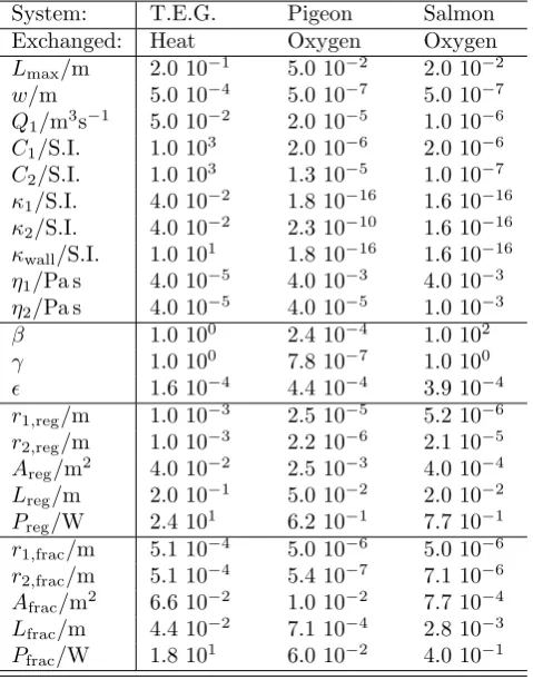
System: T.E.G. Pigeon Salmon Exchanged: Heat Oxygen Oxygen Lmax/m 2.0 10−1 5.0 10−2 2.0 10−2
w/m 5.0 10−4 5.0 10−7 5.0 10−7 Q1/m3s−1 5.0 10−2 2.0 10−5 1.0 10−6
C1/S.I. 1.0 103 2.0 10−6 2.0 10−6
C2/S.I. 1.0 103 1.3 10−5 1.0 10−7
κ1/S.I. 4.0 10−2 1.8 10−16 1.6 10−16
κ2/S.I. 4.0 10−2 2.3 10−10 1.6 10−16
κwall/S.I. 1.0 101 1.8 10−16 1.6 10−16
η1/Pa s 4.0 10−5 4.0 10−3 4.0 10−3
η2/Pa s 4.0 10−5 4.0 10−5 1.0 10−3
β 1.0 100 2.4 10−4 1.0 102 γ 1.0 100 7.8 10−7 1.0 100 1.6 10−4 4.4 10−4 3.9 10−4 r1,reg/m 1.0 10−3 2.5 10−5 5.2 10−6
r2,reg/m 1.0 10−3 2.2 10−6 2.1 10−5
Areg/m2 4.0 10−2 2.5 10−3 4.0 10−4
Lreg/m 2.0 10−1 5.0 10−2 2.0 10−2
Preg/W 2.4 101 6.2 10−1 7.7 10−1
r1,frac/m 5.1 10−4 5.0 10−6 5.0 10−6
r2,frac/m 5.1 10−4 5.4 10−7 7.1 10−6
Afrac/m2 6.6 10−2 1.0 10−2 7.7 10−4
Lfrac/m 4.4 10−2 7.1 10−4 2.8 10−3
Pfrac/W 1.8 101 6.0 10−2 4.0 10−1
Table 1: Estimated parameters for various real systems. ‘S.I.’ refers to the international system of units; so for thermal systems C will have units Jm−3K−1 and κ will have units Wm−1K−1. For gas exchange, C will have units kilogram of relevant gas per m3 of fluid, per Pascal of partial pressure, and
κwill have units kg s−1m−1Pa−1(so thatκ/Cis a diffusivity). ‘T.E.G.’ is thermo-electric generation from internal combus-tion engine exhaust (we have chosen values corresponding to a car/personal automobile). For the animal respiratory sys-tems we assume that transport across the exchange membrane is similar to that of water. For blood, we assume that oxygen can exist in a mobile form (dissolved in the water-like serum) and an immobile form (bound to haemoglobin). Thus the oxy-gen conductivityκ1 for blood is the same as for water, while
C1 is increased over that of water by the carrying capacity of haem. Data are from Refs. [14–18]. Results for a regular ex-change network are indicated by the subscript ‘reg’; while the results for the fractal exchange surfaces (denoted by a subcript ‘frac’) use a Hausdorff dimension d = 2.33. For the cases of pigeon and salmon respiration, we impose the additional con-straint that r1 >5µm, in order to allow erythrocytes to pass through. This only affects the fractal case, and without this re-quirement, the optimised value ofr1for the fractal case would be 1.5µm and 0.4µm respectively.
exchanger. Suppose that the pipes comprising the supply
135
network branch into b smaller pipes at each hierarchical
136
level k of the tree, (where pipes with higher values of k
137
are smaller, and closer to the active layer – the regular
138
array of pipes – where exchange occurs). Let the ratio of
139
pipe radii between neighbouring levels be ρ <1, and the
140
ratio of pipe lengths beλ. The ratio of power dissipated
141
between hierarchical levels is therefore 142
Pk+1/Pk =λ/(bρ4). (12)
Since the active layer is densely covered with pipes, the 143
condition to fit the supply network into space isρ≥b−1/2. 144
Therefore, provided λ > bρ4, the power will increase ex- 145
ponentially withkand the overall power dissipation in the 146
supply network will be of order that in the last layer; and 147
therefore of the same order as in the active layer. The 148
supply network will therefore not dominate the power dis- 149
sipation. 150
151
Double fractal exchange networks. – From the 152
solutions to the optimum regular exchange networks, the 153
lateral cross section A always expands to its maximum 154
valueL2
max. If this restriction were lifted, a more efficient 155
exchanger would likely be possible. This can be achieved 156
by allowing the active layer (provided it is thin enough, 157
and can still be provided with a branching supply net- 158
work) to become corrugated, while still fitting within the 159
prescribed roughly cubical volume L3max available. One 160
way to do this is to turn the active layer into an approx- 161
imation to a fractal surface. Suppose the active layer is 162
corrugated into a fractal surface over a range of lateral 163
length scales down to a scalex≥L, such that in the limit 164
x→0 the Hausdorff dimension [19] of the surface would be 165
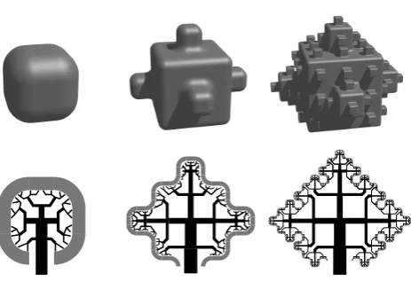
d. Fig. 2 shows schematically an example in which the sur- 166
face is the type I quadratic Koch surface with (in the limit) 167
Hausdorff dimension dkoch = ln 13/ln 3 ≈ 2.33. Let the 168
area of the active layer be A(x), whereA(Lmax) =L2max, 169
then from Hausdorff’s definition of dimension, we see that 170
A(x) = L2
max(x/Lmax)2−d. We can therefore replace the 171
inequality ˆA≤1 in eq. (10) by 172
ˆ
[image:3.595.35.275.87.393.2]A=πN1(ˆr1+ ˆw/2)2+πN2(ˆr2+ ˆw/2)2≤Lˆ2−d. (13)
Fig. 3 shows the effect of(varied through alteringQ1) on 173
the power dissipation for fractal exchangers corresponding 174
to the scenarios in table 1, compared to that of the regular 175
exchanger. Corrugating the exchange layer into a type I 176
quadratic Koch surface leads to a significant reduction in 177
the dissipated power for the two biological cases (factor 178
gain of 10 for pigeon lungs and 2 for salmon gills). How- 179
ever, the small size of the optimum pipe radiir1may mean 180
that this degree of optimization is precluded by other con- 181
siderations. For instance, erythrocytes need to be able to 182
pass through these type 1 (blood carrying) vessels. 183
184
Conclusions. – Exchange networks of the class we 185
show here exhibit broadly power-law dependence of the 186
dissipated power with the quantity(which measures the 187
required throughput: the rate of exchange of heat or gas 188
needed). This is true both for a fractally corrugated or a 189
simple regular array of exchange pipes. However, the frac- 190
tal exchangers demonstrate factor gain in efficiency when 191
for pigeon lungs and salmon gills. The exchangers exhibit
193
a crossover between regimes as a function of the required
194
throughput, where different constraints (geometrical or
195
completeness of exchange) are limiting; and if other
pa-196
rameters were changed, such as conductivities, one could
197
expect regimes in which either wall or fluid conductivity
198
would be limiting.
199
We note that the analysis we have performed here aims
200
specifically to minimise required power while ensuring
201
complete exchange has taken place. In practice, other
de-202
sign constraints may need to be included, for example a
203
requirement that the network be robust [3] or repairable
204
[20, 21] under external attack [22, 23], or the cost of
build-205
ing the network may be significant compared to its
oper-206
ating costs [24, 25].
207
REFERENCES 208
[1] Green D.W. and Perry R.H.(Editor),Perry’s Chemical
209
Engineers’ Handbook, Eighth Edition(McGraw-Hill) 2007. 210
[2] West G., Brown J.H. and Enquist B.J., Science, 211
276(5309)(1997) 122. 212
[3] Katifori E., Sz¨oll¨osi G.J and Magnasco M.O.,Phys.
213
Rev. Lett.,104(2010) 048704. 214
[4] Makanya A.N and Djonov V.,Microscopy Research and
215
Technique, 71(9)(2008) 689. 216
[5] Wiebe B.M. and Laursen H.,Microscopy Research and
217
Technique,32(1995) 255. 218
[6] Hague R. and Reeves P.,Ingenia,55(2013) 38. 219
[7] Tuckerman D.B. and Pease R.F.W., Electron device
220
letters,2(5)(1981) 126. 221
[8] Bejan A. and Errera M.R.,Fractals,5(4)(1997) 685. 222
[9] Chen Y. and Cheng P.,Int. J. Heat and Mass Transfer, 223
45(2002) 2643. 224
[10] Escher W., Michel B. and Poulikakos D., Int. J.
225
Heat and Mass Transfer,52(5-6)(2009) 1421. 226
[11] Bejan A. and Fautrelle Y.,Acta Mechanica,163(1-2)
227
(2003) 39. 228
[12] Twigg M.V., Applied Catalysis B: Environmental, 70
229
(2007) 2. 230
[13] Hagenbach E., Annalen der Physik und Chemie, 109
231
(1860) 385. 232
[14] Lide D.R.(Editor),Handbook fo chemistry and physics,
233
75th Edn(CRC Press, Inc.) 1995. 234
[15] Diffusion: Mass Transfer in Fluid Systems (2nd ed.)
Cus-235
sler E.L., (Cambridge University Press) 1997. 236
[16] Animal physiology: adaptation and environment
237
Schmidt-Nielsen K., (Cambridge University Press,
238
Cambridge) 1990. 239
[17] Butler P.J., West N.H. and Jones D.R.,Journal of
240
Experimental Biology,71(1977) 7. 241
[18] Kicenuik J.W. and Jones D.R.,Journal of
Experimen-242
tal Biology,69(1977) 247. 243
[19] Hausdorff F.,Mathematische Annalen,79(1-2)(1919) 244
157. 245
[20] Quattrociocchi W., Caldarelli G. and Scala A., 246
PLoS ONE,9(2)(2014) e87986. 247
[21] Farr R.S., Harer J.L. and Fink T.M.A., Phys. Rev.
248
Lett.,113(3)(2014) 138701. 249
[22] Cohen R., Erez K., ben-Avraham D. and Havlin S., 250
Phys. Rev. Lett.,85(2000) 4626. 251 [23] Cohen R., Erez K., ben-Avraham D. and Havlin S., 252
Phys. Rev. Lett.,86(2001) 3682. 253 [24] Bohn S. and Magnasco M.O., Phys. Rev. Lett., 98 254
(2007) 088702. 255
Lmax
Lmax
(c) (a)
(b)
area A
[image:5.595.43.272.135.291.2]Fig. 1: (a) Schematic of the geometry of a counter-current heat exchanger (‘active layer’) fitting inside a prescribed cubic volume of side length Lmax. (b) Detail of the active layer, showing a regular array of pipes carrying alternately counter-flowing streams. (c) The active layer connected to a branching and (on the other side) anastomosing fractal supply network.
Fig. 2: Top row: schematic of the active layer of fig. 1(a), cor-rugated into a hierarchical (fractal) surface, comprising (left to right) greater area and more iterations of the fractal. Bot-tom row: Schematic section through these surfaces showing the fractal supply network in the interior (the corresponding network outside is not shown, and will require a more complex design to ensure equal flow to all parts of the active layer).
-5 -4 -3 -2
log10( ε )
-8 -6 -4 -2 0 2 4
log
10
( P / W )
[image:5.595.294.495.295.441.2]TEG (regular) Pigeon (regular) Salmon (regular) TEG (fractal) Pigeon (fractal) Salmon (fractal)
Fig. 3: Plots of power dissipated in exchange for the three cases of table 1. Here we changeQ1to achieve different values of . The actual cases in table 1 are shown as symbols, and for some cases, a change of regime is observed, witnessed by a change in the slope of the line; although the curve visible in the top right part of the curve for ‘Salmon (fractal)’ are due to the constraint that blood vessels (type 1 pipes) should be large enough to carry erythrocytes (taken as the condition
[image:5.595.52.284.470.629.2]