The devil is in the detail: quantifying vocal variation in a complex, multi-levelled, and 1
rapidly evolving display. 2
3
Ellen C. Garland1 and Luke Rendell
4
School of Biology, University of St Andrews, St Andrews, Fife, KY16 9TH, UK 5
6
Matthew S. Lilley 7
SecuritEase International, Level 8, IBM Tower, 25 Victoria Street, Petone, 5012, New 8
Zealand 9
10
M. Michael Poole 11
Marine Mammal Research Program, BP 698, Maharepa, 98728, Mo’orea, French 12
Polynesia 13
14
Jenny Allen and Michael J. Noad 15
Cetacean Ecology and Acoustics Laboratory, School of Veterinary Science, 16
University of Queensland, Gatton, QLD, 4343, Australia 17
18 19
Running title: Quantifying multi-levelled vocal variation 20
Keywords: song; sequence; cultural evolution; Levenshtein distance; humpback whale 21
22 23 24
ABSTRACT 25
Identifying and quantifying variation in vocalizations is fundamental to advancing our 26
understanding of processes such as speciation, sexual selection, and cultural 27
evolution. The song of the humpback whale (Megaptera novaeangliae) presents an 28
extreme example of complexity and cultural evolution. It is a long, hierarchically 29
structured vocal display that undergoes constant evolutionary change. Obtaining 30
robust metrics to quantify song variation at multiple scales (from a sound through to 31
population variation across the seascape) is a substantial challenge. Here, we present a 32
method to quantify song similarity at multiple levels within the hierarchy. To 33
incorporate the complexity of these multiple levels, the calculation of similarity is 34
weighted by measurements of sound units (lower levels within the display) to bridge 35
the gap in information between upper and lower levels. Results demonstrate that the 36
inclusion of weighting provides a more realistic and robust representation of song 37
similarity at multiple levels within the display. Our method permits robust 38
quantification of cultural patterns and processes that will also contribute to the 39
conservation management of endangered humpback whale populations, and is 40
applicable to any hierarchically structured signal sequence. 41
42
PACS number(s): 43.80.Ka, 43.80.Ev 43
I. INTRODUCTION 50
Identifying and quantifying variation in vocalizations is fundamental to advancing our 51
understanding of processes such as speciation (Riesch et al., 2012), sexual selection 52
(Catchpole & Slater, 2008), and cultural evolution (Rendell & Whitehead, 2001; Noad 53
et al., 2000; Janik, 2014). For example, variations in the group-specific calls of killer 54
whales (Orcinus orca) are believed to be leading to speciation (Riesch et al., 2012) 55
potentially through culture-genome coevolution (Foote et al., 2016), while the vocal 56
displays of song birds are driven by both sexual selection and cultural evolution 57
(Catchpole & Slater, 2008). Understanding variation within and between habitats can 58
also support conservation and management by revealing details of population 59
structure. Therefore, robust metrics to quantify vocal variation at multiple scales 60
(from single utterances through to variation across the land and seascape) are essential 61
to address what defines a “dialect”, how dialects may correspond to populations, and 62
how this information is incorporated into the management of populations or species. 63
Substantial research has been conducted at comparing the population 64
repertoires of many species, including our own, to identify and quantify dialect 65
variation (e.g., human language: Wieling & Nerbonne, 2015; bird song: Catchpole & 66
Slater, 2008; whale song: Payne and Guinee, 1983; rock hyrax, Procavia capensis: 67
Kershenbaum et al., 2012). Studies on non-human animals typically compare call 68
types, and how the parameters of each call and frequencies with which they are used 69
vary geographically. This can become complicated when vocalizations are grouped 70
together into bouts or displays. Songbird dialects are a well-established means of 71
defining groupings (Catchpole & Slater, 2008). Dialects are defined as song 72
differences between neighboring populations of potentially interbreeding individuals 73
few to tens of syllables. In contrast, humpback whale (Megaptera novaeangliae) 75
songs can last in excess of 20 minutes and commonly comprise thousands of units 76
(individual sounds). This male-only vocal display is long, complex, and highly 77
stereotyped (Payne and McVay, 1971). 78
Humpback whale song is divided into multiple levels that are stacked on top 79
of each other (i.e., it is a nested hierarchy; Payne and McVay, 1971; Herman and 80
Tavolga, 1980). The shortest, continuous sound to our ear is called a ‘unit’ (Payne and 81
McVay, 1971; Fig. 1i). Several units are arranged in a stereotyped sequence that is 82
termed a ‘phrase’. A phrase is repeated multiple times and this is called a ‘theme’. A 83
few different themes, each comprised of repeats of a different stereotyped phrase, are 84
sung in a particular order to make a ‘song’. Songs are repeated multiple times by an 85
individual whale to comprise a ‘song session’. Different versions of the song 86
(comprised of different themes and phrases) are termed ‘song types’ (Garland et al., 87
2011). For context, humpback whale phrases and bird songs are considered analogous 88
(see Cholewiak et al., 2012). There is a clear challenge in incorporating all of this 89
variation into a quantitative analysis that includes as much information as possible 90
without abstracting from the data. 91
93
FIG. 1. Spectrograms illustrating the hierarchical structure of humpback whale song. 94
A single unit (‘trumpet’) and a single phrase from Theme 25a are shown in the top 95
panel. Theme 25a units from the single phrase in the top panel are as follows: short 96
ascending moan, grunt, grunt, grunt, grunt, grunt, grunt, short ascending moan, 97
trumpet, squeak, trumpet, squeak, trumpet. The repetition of phrases and the 98
sequential singing of themes are shown in each of the subsequent panels 99
(corresponding audio: SuppPubmm1.wav). Spectrograms were 2048 point fast Fourier 100
transform (FFT), Hann window, 31 Hz resolution, and 75% overlap, generated in 101
Raven Pro 1.4. 102
103
Within a population, most males conform to the current arrangement and 104
content of the song (Winn and Winn, 1978; Payne et al., 1983). The song 105
progressively evolves through time (Payne and Payne, 1985), with all males 106
incorporating these changes to maintain the observed similarity. Across an ocean 107
of song similarity (Payne and Guinee, 1983; Helweg et al., 1990, 1998; Cerchio et al., 109
2001). However, song sharing within the western and central South Pacific is very 110
dynamic as songs can be directionally transmitted eastward across the region from 111
eastern Australia to French Polynesia, usually over a period of two years (Garland et 112
al., 2011, 2013). The underlying drivers for this unidirectionality in song transmission 113
are not well understood, but have been suggested to be a result of differences in 114
population sizes within the region (Garland et al., 2011). Despite this transmission of 115
different versions of the display across the region, it is possible to use differences in 116
the song to identify different dialects and also populations at any point in time 117
(Garland et al., 2015). Songs and the stereotyped sequences of units therein are used 118
to define geographic dialects (Payne and Guinee, 1983; Garland et al., 2015). Since 119
variation can occur at all levels of the song structure, it is a substantial analysis 120
challenge to incorporate variation at all these levels into a single metric. 121
Many studies have undertaken quantification of humpback whale sounds 122
(units) to allow comparison, typically involving the measurement of time and 123
frequency parameters (e.g., Dunlop et al., 2007; Stimpert et al., 2011; Rekdahl et al., 124
2013). Previous work has also compared multiple metrics to establish which of a 125
variety of commonly employed sequence analysis techniques performs best for 126
comparing humpback whale song (Kershenbaum and Garland, 2015). The string edit 127
or Levenshtein distance (LD) metric outperformed all other metrics in comparing 128
humpback whale song sequences. The LD is a robust metric that should be employed 129
in the comparison of song in preference to other commonly utilized techniques (such 130
as Markov chains, hidden Markov models or Shannon entropy). The LD is a basic 131
technique in computer science and information theory which has been used in 132
and has also found favour in linguistics (e.g., Wieling and Nerbonne, 2015) and 134
animal bioacoustics (e.g., Margoliash et al., 1991; Kershenbaum et al., 2012). More 135
advanced applications of the LD have been undertaken to investigate bird song 136
dialects (e.g., Ranjard and Ross, 2007, 2008) and language relatedness (see Wieling 137
and Nerbonne, 2015), where the cost of substitution was reduced based on the 138
proportional similarity of acoustic features or phonetic similarity. The LD has also 139
previously been used to quantify song similarity in humpback whales (Helweg et al., 140
1998; Eriksen et al., 2005; Tougaard and Eriksen, 2006; Garland et al., 2012, 2013, 141
2015). These studies have compared song similarity among individuals and 142
populations in the South Pacific to understand dialect grouping; however, none have 143
employed a weighting system to better represent the complexities in song structure. 144
Here, we present a straightforward LD-based analysis method to quantify 145
stereotyped sequences of sounds that vary geographically (i.e., song dialects) at 146
multiple levels within the display. To incorporate the complexity of these multiple 147
levels, the calculation is weighted by sound unit measurements taken from lower 148
levels within the display. We use humpback whale song as an example due to its 149
inherent complexity and constant evolution. Instead of qualitatively judging unit 150
similarity as is commonly undertaken, the quantitative level of similarity as calculated 151
using a suite of variables taken directly from each unit type is an important step 152
towards a robust, reportable and repeatable quantification of humpback whale song. 153
154
II. METHODS 155
A. Calculating the Levenshtein distance (LD) and its derivatives 156
Both the conceptual understanding of the LD and its calculation is straightforward. 157
calculating the minimum number of changes (insertions, deletions and substitutions) 159
needed to convert one string into another (Levenshtein, 1966; Kohonen, 1985). The 160
Levenshtein distance (LD) is calculated by: 161
𝐿𝐷 𝑎,𝑏 = min (𝑖+𝑑+𝑠) (1)
162
where string (a) is converted into string (b) by the minimum number of insertions (i), 163
deletions (d) and substitutions (s). To ensure the output is comparable to more then a 164
single pair of strings, the LD is standardised by the length of the longest string within 165
the pair to give the Levenshtein distance similarity index (LSI), defined as: 166
𝐿𝑆𝐼 𝑎,𝑏 = 1− !"(!,!)
!"# (!"#!,!"#!) (2)
167
where the LD between strings a and b is divided by the length of the longer string of 168
the pair (see Garland et al., 2012, 2013). This produces a measure of similarity among 169
multiple sequences of varying lengths, and an overall understanding of the similarity 170
of all sequences (Helweg et al., 1998; Eriksen et al., 2005; Tougaard and Eriksen, 171
2006; Garland et al., 2012, 2013, 2015). 172
Within any set of sequences, a median, or most representative sequence, for 173
that set can be calculated. Examples of a set (or group) include all of the songs from a 174
population, all songs from a population in a particular year, repeated songs from an 175
individual, or all examples of a particular theme from all individuals within a 176
population. The string with the highest overall similarity to all other strings within the 177
group or set is found by summing all LSI scores per string. The string or sequence 178
with the highest summed LSI and thus highest similarity to all other members within 179
the group is then assigned as the ‘set median string’ (Kohonen, 1985). This provides a 180
representative string for the set that can then be used to compare among sets without 181
As noted in Kershenbaum and Garland (2015), the LD relies more on the 183
straight sequence of sound units and does not account for any hierarchy in the overall 184
structural pattern. To address this gap we propose a method of weighting changes in 185
higher levels within the song hierarchy using measurements taken directly from lower 186
levels. 187
188
B. Calculating weightings 189
1. Song recordings
190
Recordings of humpback whale song were made in Mo’orea, French Polynesia in 191
2005 using a Sony DAT TCD-D100 recorder and a hydrophone designed by John and 192
Beverly Ford of Vancouver, Canada (recorded digitally but then transferred to 193
computer by digital to analog conversion followed by re-digitizing at 44.1 kHz and 16 194
bit). Two different song types (Blue and Dark Red) were identified in the recordings 195
based on previously described songs (Garland et al., 2011, 2012, 2013). Given that 196
songs are constantly evolving through changes in the arrangement and content of 197
phrases and themes (Payne and Payne, 1985), and these differences can then be 198
transmitted to another population (Noad et al., 2000; Garland et al., 2011), identifying 199
differences between song types is essential to identify the underlying dynamics and 200
track dynamic dialect boundaries. 201
202
2. Unit measurements
203
Units, the shortest continuous sound to our ear delineated by silence (Payne and 204
McVay, 1971), were initially categorized into sound types by a human classifier 205
(E.C.G.; following Dunlop et al., 2007 classification system) as is common in 206
they sound (e.g., moan, groan, squeak) and included information on the slope (e.g., 208
ascending, modulated) and length of the call (e.g., short, long). This resulted in a fine-209
scale classification of units instead of large, variable unit categories (for example the 210
unit category ‘purr’ could be further subdivided into ‘long purr’ or ‘short purr’ based 211
on length). All units were coded for each recording. As a single song can contain 212
upwards of 1,000 units, a subset of units from each recording is measured. All units in 213
the first, full phrase of each theme in the recording were measured to provide a variety 214
of units from different themes in the song, and from different individuals for 215
comparison. This resulted in 750 measured units, a set containing multiple examples 216
of 96 unique unit types. All measured units were taken from a subset (described 217
above) of the 636 available phrases. Units were measured in Raven Pro 1.4 for 11 218
frequency and duration variables (Table I) following those outlined in Dunlop et al. 219
(2007). These measurements were taken from a spectrogram made with a 2048 point 220
fast Fourier transform (FFT), Hann window, 16 bit, 31 Hz resolution, and 75% 221
overlap. In R (R Development Core Team, 2015), this subset of measured units 222
(N=750, 96 unit types) was subjected to both Classification And Regression Tree 223
analysis (CART) and Random Forest classification. Of the 96 unit types classified by 224
CART and Random Forest, 77% and 73% (respectively) were classified in the same 225
way by the human classifier, inferring repeatability in the naming of units. Therefore, 226
all 636 phrases (which included both the qualitatively assigned units and the 750 227
measured units) were included in further analysis. 228
229
3. Turning unit measurements into a weighting system
230
To create a weighting cost or penalty between every pair of unit types (e.g., a moan or 231
mean of each variable (e.g., maximum frequency) for each unit type was calculated. 233
These were taken from the 750 measured units. The mean unit type values for each 234
variable were then transformed into z-scores to ensure all the variables were 235
comparable on the same scale. Given that we do not currently know what sound 236
features are most important to humpback whales, all variables were included in the 237
analysis in preference to reducing these to a small number of factors (e.g., through 238
Principal Components Analysis). The Euclidian distance was computed for all unit 239
types creating a single measure of distance between each pair of unit types in n-240
dimensional acoustic feature space (here, n=11 as there were 11 variables). The 241
Euclidian distance was normalized to the maximum pairwise distance (i.e., linearly) to 242
represent a value between 0 and 1, where 1 represented the largest distance (or highest 243
dissimilarity) between unit types in n-dimensional space. The linear normalized cost 244
d(x,y) is simply the Euclidian distance between the z-scores of units xi and yi, divided
245
by the maximum value of d: 246
𝑑 𝑥,𝑦 = !!(!!)!!(!!) !
!"# (!) (3)
247
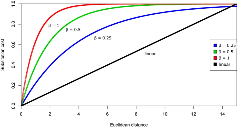
This linear normalized Euclidian distance between every unit type was used as a 248
weighting penalty for substitutions in subsequent LD calculations (Fig. 2). However, 249
preliminary tests indicated a linear scale was inadequate at capturing the differences 250
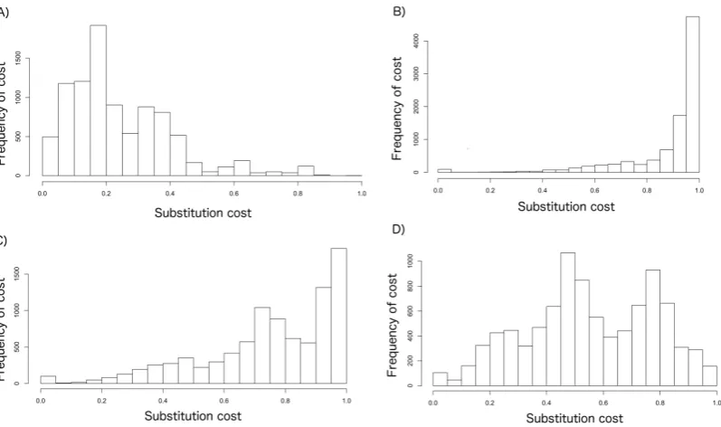
among units as the majority of penalty scores were aggregated at one end of the scale 251
due to a small number of very different units (Fig. 3). 252
To account for this, a non-linear transformation that compressed the range of 253
Euclidian distances that represent the most variation in the normalised scale was 254
undertaken. An exponential scale was able to capture the small but important 255
differences among very similar units, while also ensuring a high penalty score for the 256
𝑒𝑥𝑝_𝑐𝑜𝑠𝑡 𝑥,𝑦 =1−𝑒!!"(!,!) (4)
258
where β is the exponential coefficient. The exponential coefficient β could be altered 259
to relax the penalty slope, which resulted in a reduction in the cost for substitution 260
(Fig. 2 & 3). All initial weighting tests were run at β = 1, and then the coefficient was 261
reduced to β = 0.5 and β = 0.25 to allow the effects of weighting to be explored (Fig. 262
2). β = 1 represents the closest distribution of penalty scores to the un-weighted 263
analysis (with all scores = 1), while the relaxing of the slope to β = 0.5 and β = 0.25 264
pushes the distribution to the left (Fig. 3) into lower penalty scores. A linear 265
distribution represents the other extreme with a large number of very low substitution 266
costs (see Results for the consequences of such a situation). An alternative to our 267
weighting system not explored here would be to use a penalty matrix based on the 268
output of node weights, Euclidian distances, or Cartesian distances from a self-269
organizing map (SOM; Placer et al., 2006; Green et al., 2011). 270
[image:12.595.92.492.463.677.2]271
FIG. 2. Substitution costs with different exponential coefficients (β = 1, β = 0.5 and β
272
= 0.25) and linear scaling on the Euclidian distances calculated from sound unit 273
275
FIG. 3. Histogram of the frequency of normalized substitution costs with A) linear 276
scaling, and exponential coefficients B) β = 1, C) β = 0.5, and D) β = 0.25. Note the 277
difference in the y-axis scale. 278
279
C. Applying weightings to better capture hierarchical complexity 280
The cost of any change (insertion, deletion or substitution) was initially set to 1 (cost 281
of 1 for a change, cost of 0 for no change i.e., exactly the same unit in the same 282
position) following the traditional application of the metric. Previous qualitative 283
analyses of song variation have not been so categorical; instead, substituting a unit 284
with a similar unit was considered a less important change relative to substituting it 285
with a less similar unit (Helweg et al., 1998). This is inherently sensible as there are a 286
number of sound units that are indeed very similar. However, the quantitative level of 287
similarity as calculated using a suite of variables taken directly from each unit type is 288
used here instead of qualitatively judging this similarity to move towards a robust, 289
reportable and repeatable quantification of similarity. The penalty or cost of 290
and the exponential coefficient, β. Previous studies have shown that phrase duration is 292
one of the most stable components of humpback whale song (Cholewiak et al. 2012). 293
Therefore the cost of insertion or deletion of sounds resulting in the lengthening or 294
shortening of a phrase remains unaltered (cost remains as 1). Insertions and deletions 295
are therefore more heavily penalized than substitutions in this framework. 296
297
D. Tests using humpback whale song sequences 298
Three different analyses were undertaken to demonstrate the utility of this weighted 299
analysis in capturing the inherent multi-levelled structure and complexity within the 300
display. These can be viewed as the major steps in song quantification from lower to 301
upper levels. In each analysis, the strings used for calculating the LSI represent 302
different levels in the hierarchical song structure: 303
A. Assigning a sequence of units to a known phrase and by extension a theme. In 304
this analysis, a string represents a sequence of units. 305
B. Identifying a median unit sequence per phrase/theme. Here, a string also 306
represents a sequence of units. 307
C. Assigning a song to a song type based on the sequence of phrases (as 308
quantified from analyses A and B). In this final analysis, a string represents a 309
sequence of phrases. 310
The upper level of analysis (C.) of assigning songs to song types is run solely un-311
weighted in this instance. Weightings could be utilized to trace evolving themes (none 312
are present in the current dataset; Garland et al., 2011) by including the LSI 313
dissimilarity score for those particular themes as the penalty score. The analysis was 314
run in R (R Development Core Team, 2015) utilizing custom written code (available 315
matrix, creates median strings per group (as specified by the user; see below), 317
calculates the average LSI score within and between groups to investigate average 318
similarity and also within theme variability, and calls the hclust, pvclust and pvrect 319
packages (see Suzuki and Shimodaira, 2004) to cluster strings and calculate bootstrap 320
errors. Examples of a group include all of the songs from a population, all songs from 321
a population in a particular year, repeated songs from an individual, or all examples of 322
a particular theme from all individuals within a population. The percentage theme 323
similarity function calculates the average LSI similarity of all strings within a group 324
(e.g., population, individual, theme, etc.) to provide an understanding of the 325
variability in similarity within that group. This is also calculated among groups; 326
pairwise LSI scores calculated between all strings from two groups are averaged to 327
find the average % theme similarity between those particular groups. This 328
complements the single LSI score calculated between set medians from each group. 329
Clustering was conducted using either single or average-linkage (UPGMA) clustering. 330
Each cluster matrix was bootstrapped with multi-scale bootstrap resampling (AU) and 331
normal bootstrap probability (BP) 1,000 times to establish p-values (significance for 332
AU at p > 95% and for BP at p > 70%) and SE for each split in the tree (see Garland 333
et al., 2012 for detailed methods). Branches with high AU and BP values are strongly 334
supported by the data while lower values suggest variability in their division. As a 335
further test of how well a dendrogram represented the data, the Cophenetic 336
Correlation Coefficient (CCC) was calculated. A CCC score of over 0.8 is considered 337
high and thus a good representation of the associations within the data (Sokal and 338
Rohlf, 1962). 339
III. RESULTS 342
From 19 recordings containing three hours and 24 minutes of song, a total of 636 343
phrases (i.e., a sequence of individual sound units) were transcribed. Similar phrases 344
were qualitatively assigned to themes and song types for ease of understanding 345
(following previous analyses that qualitatively matched themes and/or assigned song 346
types using un-weighted LSI analyses; Garland et al., 2011, 2012). Sixteen themes 347
were identified; the Blue song type (Table II) contained nine themes (labelled 23 to 348
30b) with 212 phrases, and the Dark Red song type contained seven themes (labelled 349
31a to 37b) with 424 phrases. Previous qualitative assignment of these themes 350
(presented in Garland et al., 2011) provides a direct comparison of this quantitative 351
method to naïve matching tests. 352
353
A. Assigning a sequence of units to a phrase and, by extension, a theme 354
The aim of this test was to assign multiple strings of units to a phrase (and therefore a 355
theme, which represents the repetition of a stereotyped set of similar phrases). The 356
clustering of phrases into themes using both un-weighted and weighted analyses was 357
conducted for all themes for both the Blue and Dark Red song types (data not shown), 358
with similar results to those reported below. To demonstrate this, three themes were 359
chosen from the Blue song type to ensure a complex task that could also be visually 360
presented without requiring a magnifying glass. All strings from each of the chosen 361
themes were included in the analysis (N=72 phrases). Theme 28a (N=19 phrases) was 362
a long phrase that contained between nine and 20 units, made up of a possible 11 363
unique unit types (Table III). The length of a 28a phrase depended on the number of 364
repetitions of a sub-phrase (a sequence of one or more units that is sometimes 365
‘violin’ units (see Table III). Theme 30b (N=33 phrases) was shorter then Theme 28a 367
with between four and seven units, and was made up of six possible unit types (Table 368
III). None of the unit types were shared between the two themes. Theme 25a (N=20 369
phrases) contained between 11 and 20 units, and was made up of seven possible unit 370
types (Table III). The length of a 25a phrase primarily depended on the number of 371
‘grunts’ (gt; a short, low frequency unit that was repeated multiple times) sung in the 372
first sub-phrase, and whether this first sub-phrase was itself repeated (Table III). 373
Theme 25a and Theme 28a shared two unit types (ba: ‘bark’, and sq: ‘squeak’), while 374
a number of other units were very similar in their acoustic features (i.e., frequency 375
and duration measures). However, these themes are clearly different in the 376
arrangement of their units (see Fig. 1), and the selection of these two themes was 377
intentional in an attempt to confuse and identify shortcomings in the weighted 378
analysis. 379
When the analysis was run un-weighted (i.e., every substitution cost=1), 380
bootstrapping indicated three general clusters corresponding to the three themes (Fig. 381
4a). The CCC of 0.974 indicated a very good representation of the associations within 382
the data, despite some of the branches in the tree not reaching AU or BP significance. 383
The average % similarity between Themes 25a and 28a was 4%, with 0% similarity 384
between either of these themes and 30b. The analysis was then run as a weighted 385
analysis with β = 1. Average-linkage hierarchical clustering and bootstrapping 386
indicated two major branches and four general clusters were present (Fig. 4b), and the 387
dendrogram was again a very good representation of the data (CCC=0.982). The 388
average % similarity between Themes 25a and 28a rose to 33%, with similarity 389
between either of these themes and Theme 30b ranging from 4 to 6%. The weighting 390
branch (Fig. 4b) were present after bootstrapping and clustering of the weighted data, 392
as Themes 25a and 28a were subdivided at a higher level of similarity than 30b. This 393
relates to the length of strings as the LD attempts to find the minimum number of 394
changes (which is weighted towards less costly substitutions). Theme 30b contained 395
two versions based on length and thus two clusters within the overall theme: a single 396
(short) or repeated (long) ‘groan’ and ‘purr’. Given this variation is permitted and 397
considered the same Theme in qualitative assessment, this provides a guide for 398
understanding the impact of length on weighting. Alternatively, it may indicate that 399
Theme 30b should be split into two finer-scale groupings based on length (i.e., 30b 400
short and 30b long). 401
To understand the overall variability in sequences within a phrase/theme, the 402
average similarity score to all other strings within the theme set was calculated (Table 403
II, % Theme similarity). While visually the difference introduced by weighting (β = 1) 404
is subtle among these three themes, weighting has a profound effect on stabilising and 405
reducing variability within a theme. This is best seen in the increase in within theme 406
similarity for each theme (Table II, column 5). The difference between un-weighted 407
and weighted (β = 1) analyses was clear. Theme 25a increased in similarity to itself 408
(from 73% to 79%), as did Theme 28a (from 60% to 70%) and Theme 30b (from 44% 409
to 53%) from un-weighted to weighted analyses, respectively. For example, the cost 410
of substituting between two units, a ‘bark’ (ba) and a ‘long bark’ (lb), was 411
significantly reduced from cost = 1 (un-weighted analysis) to cost = 0.506 in the 412
weighted analysis (β = 1), as a long bark represents a longer duration version of a bark 413
(> 1 sec). There is a trade-off, however, between reducing variability within a theme 414
and increasing the similarity among themes. 415
417
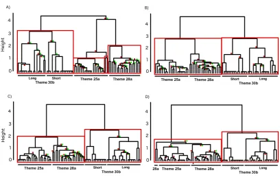
[image:19.595.93.502.95.353.2]418
FIG. 4. Dendrograms of bootstrapped (1000) LSI average-linkage hierarchical 419
clustered individual unit strings from Themes 25a, 28a and 30b (N=72) for A) un-420
weighted, B) β = 1, C) β = 0.5, and D) β = 0.25 analyses. Where multi-scale bootstrap 421
resampling (AU; left, red ) p-values and normal bootstrap probability (BP; right, 422
green ) p-values did not meet significance (p<0.95, p<0.7, respectively), these are 423
displayed (color online). Red boxes indicate clusters that are strongly supported by 424
the data. Theme 30b is split into two versions: ‘Long’ had four starting units, while 425
‘short’ contained two starting units. Note the confusion of Theme 25a and 28a in D 426
(*) indicating the process of relaxing the coefficient value has gone too far. 427
428
To further explore the impact of weighting and this trade-off, the exponential 429
coefficient was relaxed from β = 1 to β = 0.5 and β = 0.25. This reduces the steepness 430
and relaxes the penalty slope, drawing similar units closer together (Fig. 2 & 3). For 431
example, substituting from a bark to a long bark had an initial penalty of 0.506 when 432
This resulted in all themes increasing their self-similarity at each change in scale 434
(Table II). For example, Theme 30b increased its within theme similarity to 64% at β
435
= 0.25 (from 53% at β = 1, and 59% at β = 0.5). Relaxing the slope continues to 436
reduce the penalty of substitution. However, there is an obvious limit to relaxing the 437
penalty for substitution as a threshold was reached in this case where similarity in 438
phrase length overrode content of the phrase. It was less costly to substitute all units 439
then undertake any insertion or deletion operations. Using the bark/long bark example 440
above, a substitution penalty of 0.162 may allow up to six substitution operations 441
being equivalent to one insertion operation (insertion penalty cost=1). This threshold 442
was reached at β = 0.25; phrases from Theme 25a and 28a start to be mixed together 443
in a single cluster at this level of weighting (Fig. 4d). To balance the trade-off 444
between reducing within-theme variability and increasing among theme similarity in 445
the current study, the majority of substitution penalty scores needed be above 0.6 (i.e., 446
Fig. 3b & 3c) to ensure a small number of very similar sounds could be substituted 447
while the majority of sounds were costly. Investigating the distribution of penalty 448
scores (Fig. 3) allowed a visualization of the potential skew in distribution that was 449
particularly exacerbated by linear scaling (where there were a high number of 450
extremely low [<0.2] penalty scores). 451
452
B. Assigning a median unit sequence (set median) per phrase 453
Utilising all Blue song strings (N = 212 phrases, each containing a string of units), the 454
most representative unit sequence (string) for each theme was identified with and 455
without weighting. This became the set median for each theme as this string had the 456
were run four times (i.e., un-weighted, β = 1, β = 0.5, and β = 0.25), four set medians 458
were calculated for each theme. 459
The analysis was first run un-weighted to provide the initial set medians, 460
followed by weighted analyses. This provides a distinction between changes in set 461
medians arising as a result of weighting (un-weighted vs. weighted), or as a result of 462
changing the level of beta coefficient (e.g., β = 1 vs. β = 0.5). Within a theme, 463
including weighting (β = 1) resulted in a single set median string changing 464
arrangement from the un-weighted set median: Theme 27 (Table II). This theme had 465
the highest sample size (N=79), and it was also particularly variable in unit choice. 466
Weighting allowed similar units (i.e., ‘ascending’ and ‘n-shaped trills’, ti(a) and ti(n)) 467
to be substituted with a reduced penalty. Therefore, the similarity within the theme 468
increased by 19%, from 42% to 61%. 469
As above, the exponential coefficient was relaxed from β = 1 to β = 0.5 and β
470
= 0.25 to explore the impact of weighting on set median string assignment. Weighting 471
at β = 0.5 resulted in two additional themes, Themes 26b and 30b, changing their set 472
medians (Table II). Both themes were lengthened by two units, instead of being 473
represented by the more condensed version of the theme. Theme 27 did not change its 474
set median sequence from β = 1 to β = 0.5 (Table II). Themes 30b and 26b had the 475
second and third largest sample sizes in the study, respectively. When β = 0.25, 476
Theme 25a included a sixth grunt (gt) in its set median, and increased its within theme 477
similarity to 82% (from 81% at β = 0.5; Table II). Once a set median changed through 478
weighting, it remained in the new form as the exponential coefficient was further 479
relaxed. 480
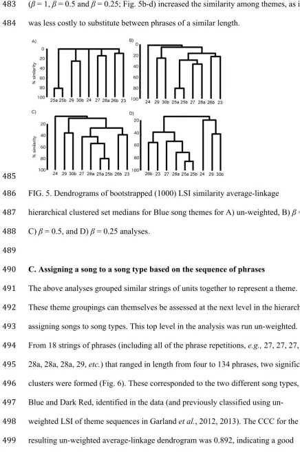
Cluster analysis of the un-weighted set median sequences indicated the 481
(β = 1, β = 0.5 and β = 0.25; Fig. 5b-d) increased the similarity among themes, as it 483
was less costly to substitute between phrases of a similar length. 484
[image:22.595.49.486.74.764.2]485
FIG. 5. Dendrograms of bootstrapped (1000) LSI similarity average-linkage 486
hierarchical clustered set medians for Blue song themes for A) un-weighted, B) β = 1, 487
C) β = 0.5, and D) β = 0.25 analyses. 488
489
C. Assigning a song to a song type based on the sequence of phrases 490
The above analyses grouped similar strings of units together to represent a theme. 491
These theme groupings can themselves be assessed at the next level in the hierarchy: 492
assigning songs to song types. This top level in the analysis was run un-weighted. 493
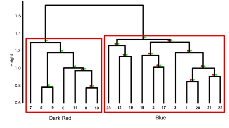
From 18 strings of phrases (including all of the phrase repetitions, e.g., 27, 27, 27, 27, 494
28a, 28a, 28a, 29, etc.) that ranged in length from four to 134 phrases, two significant 495
clusters were formed (Fig. 6). These corresponded to the two different song types, 496
Blue and Dark Red, identified in the data (and previously classified using un-497
weighted LSI of theme sequences in Garland et al., 2012, 2013). The CCC for the 498
representation of the structure within the data despite some branches not reaching AU 500
or BP significance. 501
[image:23.595.76.454.134.345.2]502
FIG. 6. Dendrogram of bootstrapped (1000) LSI average-linkage hierarchical 503
clustered strings of phrases (i.e., a song) from all recordings. Terminal node numbers 504
refer to recording number. The two clusters correspond to the two different song 505
types, Dark Red and Blue. Where multi-scale bootstrap resampling (AU; left, red ) 506
p-values and normal bootstrap probability (BP; right, green ) p-values did not meet 507
significance (p<0.95, p<0.7, respectively), these are displayed (color online). 508
509
IV. DISCUSSION 510
Here, we have shown how weighting unit substitutions when calculating sequence 511
similarities can better represent the biological reality that some sound units are more 512
similar than others in the quantitative analysis of humpback whale song. We did this 513
by incorporating direct acoustic measurements from lower levels in the song 514
hierarchy into sequence similarity calculations focussed on upper levels. There is no 515
perfect solution to such analytical challenges and no weighting scheme that will be 516
reducing the abstract nature of sequence comparisons relative to the empirical system 518
under study. We suggest that researchers think carefully about the research question at 519
hand before employing a weighting scheme. Each of the three analytical tests was 520
affected differently when weighted, resulting in varying levels of ‘success’. Given the 521
extensive previous quantification of these two song types and themes by a number of 522
different researchers (Miksis-Olds et al., 2008; Smith et al., 2008; Garland et al., 523
2011, 2012, 2013, 2015; Rekdahl et al., 2013), we considered ‘success’ in this context 524
as agreement with those previous studies – but such studies will not be available in 525
most cases. Below we review the impact of weighting on each analysis and outline 526
some potential implications and avenues for improvement. 527
528
A. Assigning a sequence of units to a phrase and, by extension, a theme 529
The clustering of the un-weighted unit sequences mirrored the previous qualitative 530
assignment of unit sequences to phrases/themes. When weighting was applied, 531
however, clustering was more defined at a higher level before reaching a tipping point 532
where different themes were merged together. Weighting will favor substitution (with 533
a cost of <1) over insertion or deletion (both cost 1), as the LD algorithm strives to 534
find the lowest cost to turn string one into string two. Therefore, phrases of similar 535
length are artificially going to be considered closer together (as was evident between 536
Themes 25a and 28a). The inclusion of two themes that were closely aligned in length 537
with a suite of potentially similar units was intentional. However, weighting 538
continued to divide these themes into two distinct clusters with no mixing of themes 539
until the coefficient was significantly relaxed (β = 0.25; Fig. 4d). This corresponded 540
to the majority of substitution costs being below 0.6 (Fig. 3), indicating a tipping 541
arrangement of themes in the song should guide the researcher in interpreting this 543
structure in the context of the research question at hand. 544
Utilizing all strings from the Blue song type, weighting resulted in clear 545
groupings of strings into phrases and themes. While un-weighted analyses do 546
represent the structure of song and should always be undertaken in the first instance, 547
weighting provides a quantitative way of making and reporting decisions about 548
‘similar units in similar locations’ to differentiate between themes more subtlety. 549
Here, we have not binned the substitution costs (e.g., 0.25 to 0.5 = cost 0.5) or 550
included a cut-off value within the cost matrix where the cost will automatically 551
change to 1. One could modify our approach by deciding that any calculated 552
Euclidian distance cost above 0.25 or 0.5, for example, represented a very different 553
suite of sounds, and thus should have a penalty of 1. Alternative cost matrices 554
generated from other analyses, such as output Euclidian or Cartesian distances among 555
nodes from a self-organising map (SOM), could also provide a representative cost 556
matrix if sound types were assigned using the SOM. 557
558
B. Assigning a median unit sequence (set median) per phrase 559
The utility of weighting is clear in this task. Here we are moving from assigning unit 560
strings (phrases) to a theme, to finding the most representative unit string for the 561
theme. If all strings are not going to be included in upper level analyses, this data-562
condensing task to find their representative is extremely important. Weighting 563
significantly increased the average within theme % of similarity, as highly similar 564
units (e.g., bark vs. long bark) could be better incorporated into the analysis. This 565
results in the analysis treating the barks as longer or shorter duration versions of 566
another similar sound type, rather than simply as separate novel types of sound. As β
decreased, no set median string reverted back to the un-weighted set median. There 568
was an interaction with sample size (N) as larger sample sizes in terms of number of 569
strings, and more variable themes (i.e., 27) switched to a new set median first, 570
followed by themes with a moderate sample size. This indicates that larger sample 571
sizes allow the underlying variability in arrangement to be captured and longer 572
phrases allow for more variability in unit sequences, and both provide more options 573
for set medians. Increasing within-theme similarity to reduce this variability is 574
desirable. 575
As β was decreased, set medians increased in length (Table II, Themes 25a, 576
26b and 30b). Weighting appears to better incorporate both the ability to quantify 577
similar units and differences in length. However, the increase in unit similarity 578
(through relaxing β) also resulted in the ‘incorrect’ placement of phrases into different 579
themes as β passed a tipping point where similarity in phrase length appeared to be 580
more important then similarity in content. This tipping point corresponded to the 581
majority of substitution costs being below 0.6. There was less and less discrimination 582
between units resulting in phrases with the same number of units being hard to 583
differentiate. It became less costly to substitute all units then undertake any insertion 584
or deletion operations. Continuing the bark/long bark example, a substitution penalty 585
of 0.162 may allow up to six substitution operations to equal one insertion operation 586
(insertion penalty cost=1). Therefore, caution and common sense is warranted when 587
applying a weighting system. 588
One application of this set median analysis is to construct median strings per 589
individual. A researcher can calculate the most representative phrase for each theme 590
(intra-individual), and then these can be put forward into comparisons among 591
This could be further explored in a way analogous to genetic studies by using 593
AMOVA type techniques (Meirmans, 2012) to compare diversity within and between 594
populations. This could also be used in intra- and inter-group comparisons to 595
quantitatively assign song (dialects). 596
597
C. Assigning a song to a song type based on the sequence of phrases 598
Phrases and themes were labelled using the assignments from lower levels. The 599
sequence or string of phrases could then be compared to assign song types. Here, we 600
utilized the raw sequence of phrases without condensing the repeated phrases down to 601
a single theme label (as in previous work; Garland et al., 2012, 2013). For example, 602
the sequence of phrases 27, 27, 27, 27, 28a, 28a, 28a, 29, 29, 30b, 30b, 30b, and so 603
on, was used instead of removing phrase repeats and condensing the sequence to 604
theme headings (e.g., 27, 28a, 29, 30b, etc.). The aim of the exercise was to assign 605
songs to song types, therefore having a variable number of repeats solely impacted the 606
strength of similarity and not the assignment to clusters in this instance (as there were 607
no shared themes). The question at hand should dictate whether phrase repeats should 608
be included or not, as the number of repeats may be impacted by behavioral context 609
(Smith, 2009). The relative strength of similarity within a song type varied due to the 610
number of phrase repeats. There was no impact to the ‘correct’ assignment of songs to 611
song types. 612
The LSI calculation at this step was un-weighted; however, a researcher 613
interested in tracing the evolution of a theme through time may assign weightings to 614
different evolutionary stages of a theme based on LSI scores. The utility to trace 615
example representing a snapshot in time from a single year, we had no evolving 617
themes but instead had two very different song types. 618
As very few species rapidly change their songs through time, establishing 619
differences between two different versions of a display (i.e., two ‘dialects’) was the 620
initial aim of this exercise to allow the technique to be widely applicable. Within a 621
season, differences in humpback whale song types can be used to identify dialect 622
boundaries and populations (Garland et al., 2015). However, the dynamic 623
transmission of song among populations results in a complex task to assign dialect 624
boundaries through time as multiple song types transit a region (see Garland et al., 625
2015). Weighting of the LD analysis will further assist in clarifying fine-scale 626
differences in songs to assign dialect and population boundaries for conservation 627
measures. 628
629
V. CONCLUSIONS 630
Here we have demonstrated that weighting the LSI analysis better incorporates the 631
variability of unit choice in the song, allowing a suite of similar units to pose little 632
penalty for substitution. The quantification of a previously qualitative process, and the 633
merging of hierarchical levels through weightings from lower levels is an important 634
step towards a robust, reportable and repeatable quantification of humpback whale 635
song. Given that humpback whale song variation among populations can be used to 636
both identify populations and assess connectivity between them (Payne and Guinee, 637
1983; Helweg et al., 1990, 1998; Cerchio et al., 2001; Garland et al., 2015), having 638
robust metrics to quantify dialect differences is essential. Understanding variation and 639
how this occurs across the seascape also underpins the application of conservation 640
humpback whale subpopulations (Childerhouse et al., 2008), from which these data 642
were sourced. Identifying and quantifying variation in vocalizations is also 643
fundamental to advancing our understanding of processes such as speciation, sexual 644
selection, and cultural evolution. 645
Humpback whale song presents an extreme example in complexity and 646
cultural evolution. It can serve as a model for complex animal vocalizations; ensuring 647
metrics that incorporate as much information with the least amount of abstraction can 648
only strengthen outcomes. The use of such sequence comparisons and weighting 649
systems using acoustic feature space are nonetheless applicable to other singing 650
species such as bowhead and fin whales, song birds, mice, and hyrax, to name a few. 651
Humpback song shows complete population-wide changes which are replicated in 652
multiple populations at a vast geographical scale (Garland et al., 2011). The level and 653
rate of this cultural transmission remains unparalleled in any other non-human animal. 654
Accurately and quantitatively tracing these changes will help in uncovering the 655
underlying drivers of these processes and thereby contribute to our understanding of 656
animal culture, vocal learning and cultural evolution, and also the roots of human 657
language and culture. 658
659
ACKNOWLEDGEMENTS 660
We thank Emma Carroll for providing valuable comments on a previous version of 661
this manuscript. Song recording in French Polynesia was conducted under permits 662
issued to M.M.P. by the Ministry of the Environment, French Polynesia. E.C.G. was 663
funded by a Royal Society Newton International Fellowship. L.R. was supported by 664
the MASTS pooling initiative (The Marine Alliance for Science and Technology for 665
Scottish Funding Council (grant reference HR09011) and contributing institutions. 667
Some funding and logistical support was provided to M.M.P. by the National Oceanic 668
Society (USA), Dolphin & Whale Watching Expeditions (French Polynesia), Vista 669
Press (USA), and the International Fund for Animal Welfare (via the South Pacific 670
Whale Research Consortium). 671
iSee supplementary material at [] for audio file (SuppPubmm1.wav) corresponding to
Fig. 1. 672
673
REFERENCES 674
Altschul, S. F., Gish, W., Miller, W., Myers, E. W., and Lipman, D. J. (1990). “Basic 675
local alignment search tool,” J. Mol. Biol. 215, 403–410. 676
Catchpole, C. K., and Slater, P. J. B. (2008). Bird Song: Biological Themes and 677
Variations, 2nd ed. (Cambridge University Press, Cambridge, UK), pp. 1–335. 678
Cerchio, S., Jacobsen, J. K., and Norris, T. F. (2001). “Temporal and geographical 679
variation in songs of humpback whales, Megaptera novaeangliae: synchronous 680
change in Hawaiian and Mexican breeding assemblages,” Anim. Behav. 62, 681
313–329. 682
Childerhouse, S., Jackson, J., Baker, C. S., Gales, N., Clapham, P. J., and Brownell Jr, 683
R. L. (2008). “Megaptera novaeangliae (Oceania subpopulation),” IUCN 684
2012, IUCN Red List of Threatened Species, Version 2012.2. Available from 685
www.iucnredlist.org (accessed April 2016). 686
Cholewiak, D. M., Sousa-Lima, R. S., and Cerchio, S. (2012). “Humpback whale 687
song hierarchical structure: historical context and discussion of current 688
classification issues,” Marine Mammal Sci. 29, E312–E332. 689
vocalizations,” Anim. Behav. 30, 297-298. 691
Dunlop, R. A., Noad, M. J., Cato, D. H., and Stokes, D. (2007). “The social 692
vocalization repertoire of east Australian migrating humpback whales 693
(Megaptera novaeangliae),” J. Acoust. Soc. Am. 122, 2893–2905. 694
Eriksen, N., Miller, L. A., Tougaard, J., and Helweg, D. A. (2005). “Cultural change 695
in the songs of humpback whales (Megaptera novaeangliae) from Tonga,” 696
Behaviour 42, 305–328. 697
Foote, A. D., Vijay, N., Ávila-Arcos, M. C., Baird, R. W., Durban, J. W., Fumagalli, 698
M., Gibbs, R. A., Hanson, M. B., Korneliussen, T. S., Martin, M. D., 699
Robertson, K. M., Sousa, V. C., Vieira, F. G., Vinař, T., Wade, P., Worley, K. 700
C., Excoffier, L., Morin, P. A., Gilbert, M. T. P., and Wolf, J. B. W. (2016). 701
“Genome-culture coevolution promotes rapid divergence of killer whale 702
ecotypes,” Nat. Commun. 7, doi:10.1038/ncomms11693. 703
Garland, E. C., Goldizen, A. W., Rekdahl, M. L., Constantine, R., Garrigue, C., 704
Daeschler Hauser, N., Poole, M. M., Robbins, J., and Noad, M. J. (2011). 705
“Dynamic horizontal cultural transmission of humpback whale song at the 706
ocean basin scale,” Curr. Biol. 21, 687–691. 707
Garland, E. C., Lilley, M. S., Goldizen, A. W., Rekdahl, M. L., Garrigue, C., and 708
Noad, M. J. (2012). “Improved versions of the Levenshtein distance method 709
for comparing sequence information in animals’ vocalisations: Tests using 710
humpback whale song,” Behaviour 149, 1413–1441. 711
Garland, E. C., Noad, M. J., Goldizen, A. W., Lilley, M. S., Rekdahl, M. L., 712
Constantine, R., Garrigue, C., Daeschler Hauser, N., Poole, M. M., and 713
understand the dynamics of song exchange at the ocean basin scale,” J. 715
Acoust. Soc. Am. 133, 560–569. 716
Garland, E. C., Goldizen, A. W., Lilley, M. S., Rekdahl, M. L., Constantine, R., 717
Garrigue, C., Daeschler Hauser, N., Poole, M. M., Robbins, J., and Noad, M. 718
J. (2015). “Population structure of humpback whales in the western and 719
central South Pacific Ocean as determined by vocal exchange among 720
populations,” Conserv. Biol. 29, 1198-1207. 721
Green, S. R., Mercado III, E., Pack, A. A., and Herman. L. M. (2011). “Recurring 722
patterns in the songs of humpback whales (Megaptera novaeangliae),” Behav. 723
Process. 86, 284-294. 724
Helweg, D. A., Herman, L. M., Yamamoto, S., and Forestell, P. H. (1990). 725
“Comparison of songs of humpback whales (Megaptera novaeangliae) 726
recorded in Japan, Hawaii, and Mexico during the winter of 1989,” Sci. Rep. 727
Cetacean. Res. 1, 1-20. 728
Helweg, D. A., Cato, D. H., Jenkins, P. F., Garrigue, C., and McCauley, R. D. (1998). 729
“Geographic variation in South Pacific humpback whale songs,” Behaviour 730
135, 1–27. 731
Herman, L. M., and Tavolga, W. N. (1980) “The communication systems of 732
cetaceans,” in Cetacean Behavior: Mechanisms and Functions, edited by L. 733
M. Herman, John Wiley (New York, USA), pp. 149–209. 734
Janik, V. M. (2014). “Cetacean vocal learning and communication,” Curr. Opin. 735
Neurobiol. 28, 60–65. 736
Kershenbaum, A., and Garland, E. C. (2015). “Quantifying similarity in animal vocal 737
sequences: which metric performs best?,” M. Ecol. Evol. 6, 1452–1461. 738
and geographical dialects in the songs of male rock hyraxes,” Proc. R. Soc. B 740
279, 2974–2981. 741
Kohonen, T. (1985). “Median strings,” Pattern Recogn. Lett. 3, 309–313. 742
Levenshtein, V. I. (1966). “Binary codes capable of correcting deletions, insertions 743
and reversals,” Dokl. Phys. 10, 707–710. 744
Margoliash, D., Staicer, C. A. and Inoue, S. A. (1991). “Stereotyped and plastic song 745
in adult indigo buntings, Passerina cyanea,” Anim. Behav. 42, 367-388. 746
Meirmans, P. G. (2012). “AMOVA-Based Clustering of Population Genetic Data,” J. 747
Hered. 103, 744-750. 748
Miksis-Olds, J. L., Buck, J. R., Noad, M. J., Cato, D. H., and Stokes, M. D. (2008). 749
“Information theory analysis of Australian humpback whale song,” J. Acoust. 750
Soc. Am. 124, 2385–2393. 751
Noad, M. J., Cato, D. H., Bryden, M. M., Jenner, M.-N., and Jenner, K. C. S. (2000). 752
“Cultural revolution in whale songs,” Nature (London) 408, 537. 753
Payne, K., and Payne, R. (1985). “Large-scale changes over 19 years in songs of 754
humpback whales in Bermuda,” Z. Tierpsychol. 68, 89–114. 755
Payne, K., Tyack, P., and Payne, R. (1983). “Progressive changes in the songs of 756
humpback whales (Megaptera novaeangliae): A detailed analysis of two 757
seasons in Hawaii,” in in Communication and Behavior of Whales, edited by 758
R. Payne, AAAS Selected Symposia Series (Westview, Boulder, CO), pp. 9– 759
57. 760
Payne, R., and Guinee, L. N. (1983). “Humpback whale (Megaptera novaeangliae) 761
songs as an indicator of ‘stocks,” in Communication and Behavior of Whales, 762
edited by R. Payne, AAAS Selected Symposia Series (Westview, Boulder, 763
Payne, R. S., and McVay, S. (1971). “Songs of humpback whales,” Science 173, 585– 765
597. 766
Placer, J., Slobodchikoff, C. N., Burns, J., Placer, J., and Middleton, R. (2006). 767
“Using self-organizing maps to recognize acoustic units associated with 768
information content in animal vocalizations,” J. Acoust. Soc. Am. 119, 3140– 769
3146. 770
R Development Core Team. (2015). “R: a language and environment for statistical 771
Computing,” R Foundation for Statistical Computing, Vienna. 772
Ranjard, L., and Ross, H. A. (2007). “A Method for Bird Song Segmentation and 773
Pairwise Distance Measure of Syllables and Songs,” Proceedings of the Fourth 774
International Conference on Bio-Acoustics 29, 185–192. 775
Ranjard, L., and Ross, H. A. (2008). “Unsupervised bird song syllable classification 776
using evolving neural networks,” J. Acoust. Soc. Am. 123, 4358-4368. 777
Rekdahl, M. R., Dunlop, R. A., Noad, M. J., and Goldizen, A. W. (2013). “Temporal 778
stability and change in the social call repertoire of migrating humpback 779
whales,” J. Acoust. Soc. Am. 133, 1785–1795. 780
Rendell, L., and Whitehead, H. (2001). “Culture in whales and dolphins,” Behav. 781
Brain Sci. 24, 309–382, discussion 324–382. 782
Riesch, R., Barrett-Lennard, L. G., Ellis, G. M., Ford, J. K. B., and Deecke, V. B. 783
(2012). “Cultural traditions and the evolution of reproductive isolation: 784
ecological speciation in killer whales?,” Biol. J. Linn. Soc. 106, 1–17. 785
Smith, J. N. (2009). “Song function in humpback whales (Megaptera novaeangliae): 786
the use of song in the social interactions of singers on migration,” unpublished 787
Ph.D. thesis, The University of Queensland, pp.1-131. 788
humpback whales, Megaptera novaeangliae, are involved in intersexual 790
interaction,” Anim. Behav. 76, 467-477. 791
Sokal, R. R., and Rohlf, F. J. (1962). “The comparison of dendrograms by objective 792
methods,” Taxon 11, 33-40. 793
Stimpert, A. K., Au, W. W. L., Parks, S. E., Hurst, T., and Wiley, D. N. (2011). 794
“Common humpback whale (Megaptera novaeangliae) sound types for 795
passive acoustic monitoring,” J. Acoust. Soc. Am. 129, 476–482. 796
Suzuki, R., and Shimodaira, H. (2004). “An application of multiscale bootstrap 797
resampling to hierarchical clustering of microarray data: how accurate are 798
these clusters?,” Poster presented at the 15th Annual International Conference 799
of Genome Informatics, Posters and Software Demonstrations. Yokohama, 800
Japan. (http://www.is.titech.ac.jp/~shimo/pub/GIW2004/suzukiGIW2004.pdf) 801
Tougaard, J., and Eriksen, E. (2006). “Analysing differences among animal songs 802
quantitatively by means of the Levenshtein distance measure,” Behaviour 143, 803
239–252. 804
Wieling, M., and Nerbonne, J. (2015). “Advances in Dialectometry,” Annu. Rev. 805
Linguist. 1, 243-264. 806
Winn, H. E., and Winn, L. K. (1978). “The song of the humpback whale Megaptera 807
novaeangliae in the West Indies,” Mar. Biol. 47, 97–114. 808
815 816 817
TABLES 818
TABLE I. Variables measured for each unit. 819
Measurement Description
Duration (s) Vocalization length
Minimum frequency (Hz) Minimum frequency Maximum frequency (Hz) Maximum frequency Start frequency (Hz) Start frequency
End frequency (Hz) End frequency
Frequency range (as ratio) Max freq/min freq Frequency trend (as ratio) Start freq/end freq
Bandwidth (Hz) Max-min freq
Inflections Number of reversals in slope
Peak frequency (Hz) Frequency of the spectral peak
Pulse rate (/s) for pulsative sounds
828 829
TABLE II. Set medians from the Blue song type with and without weighting. N is the 830
number of strings for each theme present in the data. Weight is un-w = un-weighted, β
831
= 1 is the default weight of exponential coefficient, β = 0.5 is weighted to relax the 832
exponential coefficient to 0.5, and β = 0.25 is weighted to relax the exponential 833
coefficient to 0.25 (see Fig. 2). Sum similarity is the highest summed similarity score 834
of a string within the set. This string became the set median string. Note the set 835
median can change in arrangement between each of the four analyses (un-weighted, β
836
= 1, β = 0.5 and β = 0.25). % Theme similarity is the average LSI similarity of all 837
strings to all other strings within the theme. Differences between the weighted and un-838
weighted set median sequences are underlined. Each letter or combination of letters 839
represents a unit type*. A comma separates units. 840
Theme N Weight Sum
similarity
% Theme
similarity
Set median unit string/sequence
23 1 un-w 1.00 100 w, dws, w, nws, w, dws, w, dws, w, modws, be
β = 1 1.00 100 w, dws, w, nws, w, dws, w, dws, w, modws, be
β = 0.5 1.00 100 w, dws, w, nws, w, dws, w, dws, w, modws, be
β = 0.25 1.00 100 w, dws, w, nws, w, dws, w, dws, w, modws, be
24 19 un-w 13.96 62.2 as/aws, as/aws, as/aws, e
β = 1 14.13 64.8 as/aws, as/aws, as/aws, e
β = 0.5 14.24 67.1 as/aws, as/aws, as/aws, e
β = 0.25 14.363712 69.5 as/aws, as/aws, as/aws, e
25a 20 un-w 16.15 73.4 am(s), gt, gt, gt, gt, gt, am(s), t, sq, t, sq, t
β = 1 16.83 78.9 am(s), gt, gt, gt, gt, gt, am(s), t, sq, t, sq, t
β = 0.5 17.05 80.8 am(s), gt, gt, gt, gt, gt, am(s), t, sq, t, sq, t
β = 0.25 17.21 82.0 am(s), gt, gt, gt, gt, gt, gt, am(s), t, sq, t, sq, t
*Unit names: am=ascending moan, am(pul)=pulsative ascending moan, am(s)=short ascending moan, 841
as/aws=ascending shriek/ascending whistle, ba=bark, be=bellows, c=croak, c(w)=croak-whoop, 842
dws=descending whistle, e=e-sound, gr=groan, gr/gw=groan/growl, gt=grunt, lb=long bark, 843
mods=modulated shriek, modws=modulated whistle, nws=n-shaped whistle, p=purr, p(ch)=chainsaw 844
purr, s=siren, sq=squeak, sq-ds=squeak-descending shriek, t=trumpet, ti(a)=ascending trill, ti(n)=n-845
shaped trill, um=u-shaped moan, v=violin, w=whoop. 846
847 848 849
β = 1 1.83 91.7 am(s), gt, gt, gt, gt, gt, am(s), t, sq, t, sq, t, sq, t, mods
β = 0.5 1.83 91.7 am(s), gt, gt, gt, gt, gt, am(s), t, sq, t, sq, t, sq, t, mods
β = 0.25 1.83 91.7 am(s), gt, gt, gt, gt, gt, am(s), t, sq, t, sq, t, sq, t, mods
26b 28 un-w 14.86 37.1 s, am, um, modws, um, modws, um, modws
β = 1 15.77 43.1 s, am, um, modws, um, modws, um, modws
β = 0.5 17.74 52.2 s, am, um, modws, um, modws, am, modws, um, modws
β = 0.25 20.13 63.0 s, am, um, modws, um, modws, am, modws, um, modws
27 79 un-w 44.87 41.8 lb, ba, ti(a), sq-ds, ti(a), sq-ds, ti(a), sq-ds, ti(a), sq-ds
β = 1 57.60 60.6 lb, ba, ti(a), sq-ds, ti(n), sq-ds, ti(a), sq-ds, ti(n), sq-ds
β = 0.5 63.81 71.2 lb, ba, ti(a), sq-ds, ti(n), sq-ds, ti(a), sq-ds, ti(n), sq-ds
β = 0.25 68.92 80.3 lb, ba, ti(a), sq-ds, ti(n), sq-ds, ti(a), sq-ds, ti(n), sq-ds
28a 19 un-w 13.89 60.2 lb, ba, am(pul), v, v, v, am(pul), v, v, v, am(pul), v, v, v
β = 1 15.19 70.3 lb, ba, am(pul), v, v, v, am(pul), v, v, v, am(pul), v, v, v
β = 0.5 15.81 75.5 lb, ba, am(pul), v, v, v, am(pul), v, v, v, am(pul), v, v, v
β = 0.25 16.27 79.5 lb, ba, am(pul), v, v, v, am(pul), v, v, v, am(pul), v, v, v
29 11 un-w 7.85 61.4 be, c, c, c
β = 1 7.85 62.3 be, c, c, c
β = 0.5 7.88 63.3 be, c, c, c
β = 0.25 8.13 66.5 be, c, c, c
30b 33 un-w 16.52 44.0 gr/gw, p(ch), c(w), c
β = 1 18.52 53.0 gr/gw, p(ch), c(w), c
β = 0.5 20.10 58.5 gr, p, gr, p, c, c