rsos.royalsocietypublishing.org
Research
Cite this article:Walton E, Casey C, Mitsch J,
Vázquez-Diosdado JA, Yan J, Dottorini T, Ellis KA, Winterlich A, Kaler J. 2018 Evaluation of sampling frequency, window size and sensor position for classification of sheep behaviour.
R. Soc. open sci.5: 171442.
http://dx.doi.org/10.1098/rsos.171442
Received: 22 September 2017 Accepted: 8 January 2018
Subject Category:
Biology (whole organism)
Subject Areas:
behaviour/pattern recognition/bioengineering
Keywords:
sheep behaviour, classification algorithm, accelerometer and gyroscope, sensor, signal processing, precision livestock monitoring
Author for correspondence:
Jasmeet Kaler
e-mail:[email protected]
Electronic supplementary material is available online at https://dx.doi.org/10.6084/m9. figshare.c.3985326.
Evaluation of sampling
frequency, window size
and sensor position for
classification of sheep
behaviour
Emily Walton
1
, Christy Casey
2
, Jurgen Mitsch
1,3
, Jorge
A. Vázquez-Diosdado
1
, Juan Yan
1,4
, Tania Dottorini
1,3
,
Keith A. Ellis
5
, Anthony Winterlich
2
and Jasmeet Kaler
1
1School of Veterinary Medicine and Science, University of Nottingham,
Sutton Bonington Campus, Leicestershire LE12 5RD, UK
2DXC Technology, Ballybrit Business Park, Galway City H91 WP08, Ireland
3Advanced Data Analysis Centre (ADAC), School of Veterinary Medicine and Science,
University of Nottingham, Sutton Bonington Campus, Leicestershire LE12 5RD, UK 4School of Computer Science, University of Manchester, Manchester M13 9PL, UK
5Internet of Things Systems Research, Intel Labs, Leixlip W23 CX68, Ireland
JK,0000-0002-3332-7064
Automated behavioural classification and identification
through sensors has the potential to improve health and welfare of the animals. Position of a sensor, sampling frequency and window size of segmented signal data has a major impact on classification accuracy in activity recognition and energy needs for the sensor, yet, there are no studies in precision livestock farming that have evaluated the effect of all these factors simultaneously. The aim of this study was to evaluate the effects of position (ear and collar), sampling frequency (8, 16 and 32 Hz) of a triaxial accelerometer and gyroscope sensor and window size (3, 5 and 7 s) on the classification of important behaviours in sheep such as lying, standing and walking. Behaviours were classified using a random forest approach with 44 feature characteristics. The best performance for walking, standing and lying classification in sheep (accuracy
95%, F-score 91%–97%) was obtained using combination
of 32 Hz, 7 s and 32 Hz, 5 s for both ear and collar sensors, although, results obtained with 16 Hz and 7 s window were
comparable with accuracy of 91%–93% andF-score 88%–95%.
Energy efficiency was best at a 7 s window. This suggests that sampling at 16 Hz with 7 s window will offer benefits in a real-time behavioural monitoring system for sheep due to reduced energy needs.
2
rsos
.ro
yalsociet
ypublishing
.or
g
R.
Soc
.open
sc
i.
5
:1
71442
...
1. Introduction
Recent advances in sensor and smart computing technologies such as global positioning (GPS) trackers, location sensors, proximity loggers, accelerometers, gyroscopes and magnetometers have allowed researchers to study and enrich our understanding of animal movements, space-use patterns, physiology,
social interactions and the environment they inhabit [1–4]. These smart technologies have a huge
potential to inform resource management and conservation [1,3,4]. One sector that is expected to have
a considerable benefit from the use of such technologies is animal welfare and livestock agriculture
production [4] as these technologies can give insight into animal behaviour patterns and also allow
producers to monitor animals frequently to inform on farm decision making. An accurate and precise behavioural monitoring system could potentially detect behavioural changes correlated to health and welfare status changes in sheep. For example, abnormal postures and the avoidance of specific
behaviours can be used to detect foot lesions [5–7]. Similarly, lameness, a widespread welfare problem
in sheep farming around the world, will change an animal’s normal stance or gait and will also alter
behavioural activity [8,9].
Embedded and wearable devices encompassing accelerometer and gyroscope sensors have been
used widely to discriminate different behaviours in pets [10] and farm animals [11–15]. Usage of
such devices has increased as the technologies have become not only smaller, lighter and cheaper but also capable of processing, exchanging and transmitting an increasingly larger amount of information with a broad range of communication protocols. Such a large amount of data is ideally suited to be processed through machine learning, providing ideal foundations to the development of a new era of intelligent veterinary medicine and science, ultimately contributing to better animal welfare, with significant economic and ecology repercussions. Currently, various machine learning solutions (e.g. support vector machines, decision trees, Kalman filters) have been used on accelerometer data to classify behaviours such as feeding, standing, lying, ruminating, walking and standing
in cows [11–13]. In contrast to the large number of automatic behaviour classification studies
in cattle, very few studies (with varying results) have been done in sheep using sensor-based
technologies [16–18].
There are various factors, such as sampling frequency, window sizes and position of sensor that can
affect performance of classification of behaviour using accelerometer and gyroscope data [19]. This is
one possible explanation for the varying behaviour classification performance results that have been documented in literature so far for livestock behaviour classification. While there are studies in literature
evaluating these aspects for human activity classification with accelerometer data [20–22] there are no
studies in precision livestock monitoring that have simultaneously evaluated the impact of these factors on livestock behaviour classification. Often these characteristics are rarely and vaguely described in animal behaviour studies with use of choice of sampling frequency, or position and window size without any robust scientific evaluation.
Moreover, to eventually deliver a complete framework that can efficiently monitor in real time and for long durations, an understanding of the effect of sampling frequencies, sensor positions and window sizes is required. For example, cloud-based systems require real-time streaming of data to a server,
which results in a high power drain and reduced battery life [3,23]. An architectural alternative solution
to overcome high power demands on the system is the use of embedded based architecture [15,23],
where the processing can be performed on the devices attached to the animals. Nevertheless, embedded systems have their own constraints as there is limited processing power and memory on each device. Therefore, to overcome processing power limitations in embedded systems it is necessary to identify methods that optimize the available resources on such devices. A well-informed decision on optimum sampling rate, window sizes and sensor position can result in considerable improvements in energy transmission bandwidth and storage capacity.
3
rsos
.ro
yalsociet
ypublishing
.or
g
R.
Soc
.open
sc
i.
5
:1
71442
...
2. Material and methods
2.1. Study site and animals
Before starting the main trial, a pilot study for 2 days was conducted to check the research protocols described below. Ethical permission was obtained for the School of Veterinary Medicine and Science, University of Nottingham. For the main trial in this study, data were collected for 8 days from 5 October 2016 to 7 October 2016 and from 10 October 2016 to 14 October 2016. A total of six sheep were selected via stratified random sampling (age) from a flock of 140 animals at the University of Nottingham. Assessment of body condition score, age and breed was done at day 1. Body condition scoring of sheep is simply a means of assessing the degree of fatness or condition of the living animal and was scored
using UK industry guidelines [24,25]. The selected sheep had various body condition scores ranging
from 2.5 to 4 and an age ranging from 18 months to 4 years. The breeds of sheep were Texel cross (three individuals), Suffolk cross (one individual) and Mule (two individuals). Sheep were kept in a rectangular 0.3 acre field with a 179.3 m perimeter during the day, when recordings were taking place. At night, sheep were allowed into a larger 2.1 acre field until the next morning’s recordings. To facilitate individual identification, sheep were sprayed with coloured livestock spray on either side of the sheep’s body with a number between 1 and 19. Numbers sprayed on the sheep were re-sprayed again on day 5 of the trial.
2.2. Data collection
Sensor data were collected using a custom-made wearable device based on the Intel® Quark™ SE
microcontroller C1000. The device encompassed flash memory, a low-power wide-area radio module and
Bosch BMI160 integrated (Bosch-sensortec.com, 2016),±8g, low-power inertial measurement unit (IMU),
featuring a 16 bit triaxial gyroscope and a 16 bit triaxial accelerometer. The devices were of dimension
31.6×35×9 mm and weighed 4 g. The devices were attached to a lightweight Li–Po battery 270 mA h
Li-ion battery. The devices where designed for edge-based data processing, classification and reduced transmission. Although at this stage much of the functionality was unutilized and the units where used solely for data acquisition.
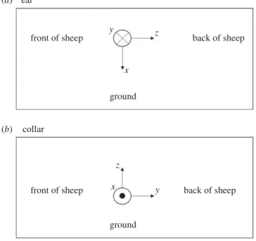
The devices were attached to six sheep at two locations (a) to the existing electronic identification ear tag via a tape and lightweight plastic tie and (b) to neck collar using tape and lightweight plastic tie. All
ear-mounted devices were fixed using the orientation illustrated infigure 1a, whereas all collar-mounted
devices were fixed using the orientation shown infigure 1b.
Devices were mounted on sheep at the beginning of each trial day at approximately 09.00 and removed the following morning at 09.00, with the exception Friday, 7 October 2016, when the devices were removed at 16.00 to prevent any possible damage over the weekend when no camera recording took place.
In this study, the device sensors were set to collect data at sampling frequencies of 8, 16 and 32 Hz per axis and each sheep was used for multiple sampling frequencies on different days. Sampling frequencies were set at the beginning of each day, and the setting remained fixed for the entire day of the recording. The devices attached to sheep were set to keep recording raw accelerometer and gyroscope data, with no energy optimization, e.g. sleep features etc. used, until either: the device storage was full or the devices
ran out of battery. Different sampling rates had a different drain on battery life [26]. Hence, sampling
frequencies of 8, 16 and 32 Hz resulted in raw data with duration of 20, 10 and 5 h, respectively. Each day sensors were prepared by first setting the sampling frequency, then switching them on, while annotating the switching time. Afterwards, to allow time synchronization with the videos, sensors were shaken for 30 s and the start time of the shaking time was annotated. This was followed by a procedure to establish a time reference, where sensors were held horizontally for 30 s and finally held vertically for 30 s. At the end of the 30 s of holding them vertically, the time was annotated. After this procedure, sensors were mounted on sheep. The recorded data were downloaded from the devices.
After removing spurious datasets due to sensor malfunction or other data retrieving issues, a total of
30 datasets (98% of the data collected) from six sheep were used for analysis.Table 1gives an overview
of the total number of datasets collected from ear and collar sensors for different sampling rates.
2.3. Behavioural observations
4
rsos
.ro
yalsociet
ypublishing
.or
g
R.
Soc
.open
sc
i.
5
:1
71442
...
ear (a)
(b)
front of sheep
front of sheep
y z
x
y z
x
back of sheep
back of sheep ground
ground collar
Figure 1.Sensor orientation for ear and collar.
Table 1.Datasets types. Number of successfully extracted datasets from six different sheep for ear and collar sensors according to
sampling frequency.
ear collar total
8 Hz 5 5 10
. . . .
16 Hz 7 7 14
. . . .
32 Hz 3 3 6
. . . .
UHS-1SD card to store the footage. The video camera was set to record in a MP4 50M format with 1080p
(1920×1080 pixels) quality. With these settings, one SD card could store 3 h and 6 min of footage. Video
recording was started each morning immediately after the installation of the first sensor and the starting time of the recording was registered. Video footage was recorded each day in the morning with duration of approximately 2 h. In the recording sessions, the starting and ending times of the recording were annotated.
2.3.1. Behaviours annotation of the videos
Time stamped video recordings of the sheep were processed using the Noldus Observer XT 11(Noldus)
(www.noldus.com) software. Coding of the video recordings into the different behavioural categories or
classes was performed by playing each video and manually pressing the corresponding code key of the identified behaviour from the set of predefined ones. Behaviours were defined based on the behaviour
ethogram developed in a pilot study where sheep were observed and in other literature [18]. Behaviours
of interest for this study can be identified according totable 2.
2.4. Data processing
Processing of the data was performed using dedicated software written in Python 3.5 [27], specifically
for this project. First, the raw sensor data (accelerometer and gyroscope) and the behaviour information from the video transcripts were aligned using the time stamps. Afterwards each file was discretized into windows of equal length. In this study, window sizes of 3, 5 and 7 s were explored, with a 50% overlap
between two consecutive windows [16,19]. During coding of the video recording an individual class label
5
rsos
.ro
yalsociet
ypublishing
.or
g
R.
Soc
.open
sc
i.
5
:1
71442
...
Table 2.Definition of sheep behaviours for classification. Different behaviours in sheep used in the classifier according to the ethogram
developed.
behaviour states description
walking sheep moves forward in a four beat motion for 2 s or more with the head up and orientated in the direction of movement
. . . .
standing sheep is standing on their four legs with or without jaw movement, head up or down
. . . .
lying sheep lying on ground in sternal or lateral recumbency with or without jaw movement, could be ruminating or
in the process of regurgitating a bolus
. . . .
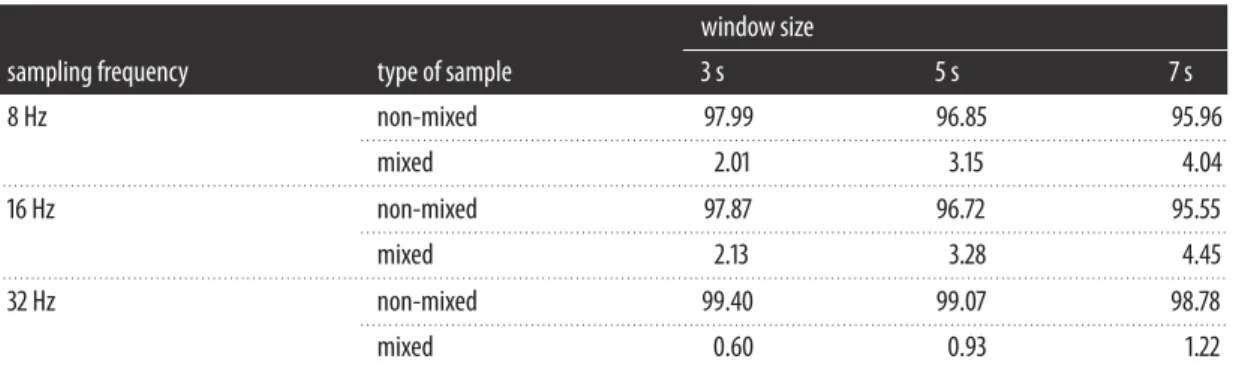
Table 3.Percentage of non-mixed and mixed windows. Summary of the percentage of samples that are non-mixed or mixed for the
three different sampling frequencies (8, 16 and 32 Hz) and for the three window sizes (3, 5 and 7 s).
window size
sampling frequency type of sample 3 s 5 s 7 s
8 Hz non-mixed 97.99 96.85 95.96
. . . .
mixed 2.01 3.15 4.04
. . . .
16 Hz non-mixed 97.87 96.72 95.55
. . . .
mixed 2.13 3.28 4.45
. . . .
32 Hz non-mixed 99.40 99.07 98.78
. . . .
mixed 0.60 0.93 1.22
. . . .
samples within a window shared the same activity class, the collective label for the entire window was set to that particular activity class. Windows that contained data points with more than one activity class label were labelled as ‘mixed’ windows and the predominant label was used as the class. The percentage of samples for the ‘mixed’ and ‘non-mixed’ windows in each of the sampling frequencies and window
sizes in this study, is shown intable 3.
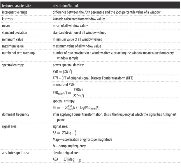
For each time window a set of feature characteristics [28] was extracted from the magnitude of the
acceleration and the magnitude of the gyroscope which are defined as follows: ¯
A=
A2
x+A2y+A2z,
¯
G=
G2x+G2y+G2z,
where Ax, Ay, Az, Gx, Gy, Gz represent the acceleration and gyroscope signals at the axes x, y, z,
respectively. Eleven different feature characteristics were extracted from both the magnitude of the
acceleration and from the magnitude of the gyroscope based on previous literature work [29,30]. In
addition, the same feature characteristics were computed from the rate of change of the magnitude of the acceleration and from rate of change of the magnitude of the gyroscope, yielding a total of 44 features that were used in the classification.
Table 4shows the 11 feature characteristics used for the classification. These include mean, standard
deviation, kurtosis, minimum and maximum value [11], interquartile range [31], signal area, absolute
signal area, number of zero crossings, dominant frequency [29] and spectral entropy [32].
2.5. Classification algorithm
Random forests [33,34] are a type of ensemble learning method that is formed through the combination of
multiple decision trees trained on the training set. When applied to the test dataset, the predictions of the individual tree models within the random forest are combined into an overall classification decision, e.g. through means of a majority vote or through the application of weights. Because of this, random forest
models correct overfitting to the training set and provide a more robust classification performance [35].
A random forest learning algorithm was implemented using Microsoft Azure Machine Learning Studio
software [36] and the set of feature characteristics previously described. The random forest algorithm
6
rsos
.ro
yalsociet
ypublishing
.or
g
R.
Soc
.open
sc
i.
5
:1
71442
...
Table 4.Feature characteristics. Feature characteristics computed for each individual window. Herefrepresents the signal andfsthe
sampling frequency.
feature characteristics description/formula
interquartile range difference between the 75th percentile and the 25th percentile value of a window
. . . .
kurtosis kurtosis calculated from window values
. . . .
mean mean of all window values
. . . .
standard deviation standard deviation of all window values
. . . .
minimum value minimum value of all window values
. . . .
maximum value maximum value of all window value
. . . . number of zero crossings number of zero crossings in a window after subtracting the window mean value from every
window sample
. . . .
spectral entropy power spectral density:
PSD= |X(f)2|
. . . . X(f)– DFT of original signal. Discrete Fourier transform (DFT)
. . . . normalized PSD:
PSDnorm(f)= PSD(f) ΣPSD(f)
. . . . spectral entropy:
SE= −ΣPSD
norm(f)·log(PSDnorm(f))
. . . . dominant frequency after applying Fourier transformation, this is the frequency at which the signal has its highest
power
. . . .
signal area signal area:
SA=ΣMag·fs1
Mag—acceleration or gyroscope magnitude
fs—sampling frequency
. . . .
absolute signal area absolute signal area:
ASA=Σ|Mag| ·fs1
. . . .
Data were split into a training set and a test set. The training dataset consisting of 70% of the full dataset was used to develop the model, while the test dataset consisting of the remaining 30% of the
original dataset was used for model evaluation and validation [37,38]. The partitioning between training
and testing data was carried out using random stratification to ensure that the ratios of the three main activities (walking, standing and lying) remained the same in both datasets.
2.5.1. Performance of the classification
The performance of the random forest classification was evaluated using the following metrics: overall
accuracy, precision, recall (also known as sensitivity),F-score and specificity, which can be computed as
follows:
Overall accuracy= TP+TN
TP+TN+FP+FN,
Precision= TP
TP+FP,
Recall= TP
TP+FN,
F−score=2·precision ·recall
precision + recall
and Specificity= TN
7
rsos
.ro
yalsociet
ypublishing
.or
g
R.
Soc
.open
sc
i.
5
:1
71442
...
where TP (true positives) is the number of instances where the behaviour of interest (walking, standing or lying) was correctly classified by the algorithm and visually observed. FN (false negatives) is the number of instances where the behaviour of interest was visually observed but was incorrectly classified as some other behaviour by the algorithm. FP (false positives) is the number of instances the behaviour of interest was incorrectly classified by the algorithm but not observed. TN (true negative) is the number of instances where the behaviour of interest was correctly classified as not being observed.
2.5.2. Precision, recall,
F-score and specificity
A more detailed comparison of the performance of the classification for each individual behaviour can be
provided by performance measures such as: precision, recall,F-score and specificity, which are computed
from the confusion matrix. In this type of matrix, each column represents the behaviour predicted by the classifier while each row represents the observed behaviour. In the electronic supplementary material, we provide the full set of confusion matrices using the random forest algorithm with 3, 5 and 7 s window sizes, for all sampling frequencies (8, 16 and 32 Hz), for both the ear-mounted and collar-mounted sensor. The overall accuracy represents the total number of correct classifications across all classes. This can be useful when the importance of correctly classifying a specific class is equal for all classes, and provides a meaningful indication of classifier performance, if the dataset is balanced, i.e. all classes are equally represented in the dataset. If one or more classes are of particular interest to the observer (e.g. walking), and the priority is to correctly classify a specific class (possibly at the cost of achieving worse performance for the other classes), precision, recall and specificity give a more in-depth representation of a classifier’s
performance. TheF-score gives a measure of a test’s accuracy and is a harmonic mean of precision and
recall. It reaches its best score at 1 and worst score at 0 [39].
To measure the level of agreement between the classifier based on ear data and the classifier based
on collar data, a Cohen’s weightedκstatistic was conducted [40]. The Cohen’s weightedκmeasure was
obtained for the three sampling frequencies (8, 16 and 32 Hz) and the three window sizes (3, 5 and 7 s).
2.5.3. Energy consumption
When considering algorithm implementation, the question of sampling frequency and window size impacting on the energy budget is important, and more specifically what trade-offs if any might be needed in terms of acceptable accuracy versus battery life. Increasing the sampling rate obviously increases the energy required to sample. For example, with respect to the inertia measurement unit (IMU) used and the specific IMU configuration/optimization applied, the difference between 16 and 32 Hz would be approximately 10 µA h versus approximately 17 µA h, or 3.08 years of battery life versus 1.81 years (assuming a 270 mA h battery). So if accuracy at 16 Hz or lower is comparable to 32 Hz there is an obvious gain in using the lower sampling rate.
We calculated the effect on energy consumption when using a 3, 5 and 7 s window size on the device
(Intel®). The device has two modes of operation ‘raw data capture’ and ‘classification’. When in raw data
capture mode the concept of window size does not apply and the device sample rate is constant at the rate chosen. In this mode the device processor persists acquired samples to memory at a constant rate, hence energy consumption is constant. Window size does apply when in classification mode (i.e. classifying using algorithm). When viewed at a window level much is changing, but to more accurately compare windows one must compare across a normalized time span, e.g. on a per hour basis. For example if raw data were captured at 16 Hz, then the input to the classification pipeline remains at 16 Hz and as such its energy consumption is constant (i.e. the IMU energy consumption is the same per hour regardless of window size). Additionally, when viewed on an hourly basis the total bytes pre-processed and classified is constant and so the ‘data processing’ energy consumption is equal. What varies when normalized is the number of times the processor acquires (reads) samples (not the total number of samples) and the number of times it persists (writes) a classification record to memory.
3. Results
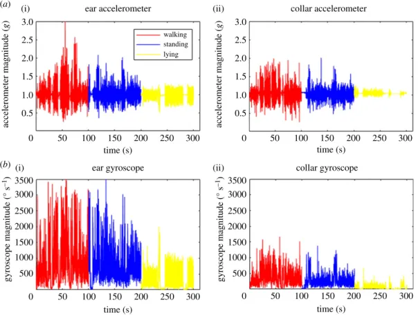
Figure 2 illustrates an example time series of the accelerometer and gyroscope magnitude output
for observed periods of lying, standing and walking recorded by ear (figure 2a(i),b(i)) and collar
(figure 2a(ii),b(ii)) sensors. The sampling frequency for both ear and collar infigure 2was 16 Hz. From
figure 2, it is very clear that is easy to discriminate between lying and any other behaviour due to
8
rsos
.ro
yalsociet
ypublishing
.or
g
R.
Soc
.open
sc
i.
5
:1
71442
...
ear accelerometer 3.0
2.5
2.0
1.5
1.0
0.5
0
3500 3000
2500
gyroscope magnitude (° s
–1
)
2000
1500
1000
500
0
3500 3000
2500
gyroscope magnitude (° s
–1
)
2000
1500
1000
500
0
50 100 150 200 250 300
50 100 150
time (s)
200 250 300
50 100 150 200 250 300
accelerometer magnitude (
g
) 3.0
2.5
2.0
1.5
1.0
0.5
0
accelerometer magnitude (
g
)
collar accelerometer
walking standing lying
50 100 150
time (s)
time (s) time (s)
200 250 300
ear gyroscope collar gyroscope
(a) (i)
(b) (i)
(ii)
(ii)
Figure 2.Representative examples of accelerometer and gyroscope data. Accelerometer (a) and gyroscope (b) data collected for collar
and ear mounted sensors with lameness score 0. Colours red, blue and yellow represent walking, standing and lying respectively. Acceleration is ing(9.81 m s−2) units.
and walking behaviours look visually similar, although the walking activity produces higher overall magnitudes for acceleration compared with standing for both collar and ear datasets.
Similar to the observations in the accelerometer data, it is easy to discriminate lying from the other two behaviours using the gyroscope magnitude as they are lower compared with lying and standing
(figure 2b). Walking also has the highest gyroscope magnitudes as observed in the accelerometer
magnitudes. Gyroscope magnitudes for ear data are different to those obtained from collar data, with amplitudes being much larger than their collar counterparts. This is another effect of the much higher overall freedom of movement of the ear sensor compared with the collar sensor. However, the three behaviours are visually distinguishable and consistent with the accelerometer observations.
3.1. Assessment of overall classification performance
3.1.1. Overall accuracy
An initial comparison of the performance of the classification across all the window sizes and sampling frequencies can be provided using values of the overall accuracy for both ear- and collar-mounted
sensors, as summarized intable 5.
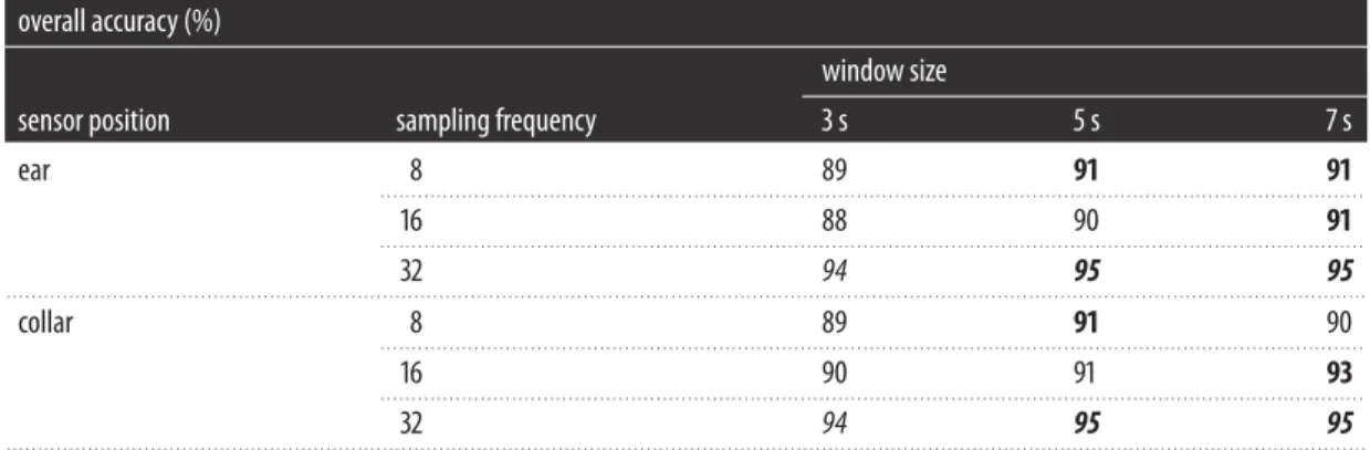
The highest overall accuracy is 95%, which was obtained for both ear and collar data at 32 Hz with 5 and 7 s windows. The lowest overall accuracy of 89% was obtained for ear data at a sampling frequency of 16 Hz with 3 s window size, and for collar data the lowest accuracy was 89% at a sampling frequency of 8 Hz with 3 s window size. Overall, the accuracies observed were the worst for 3 s windows and best for 7 s windows. For ear data, the differences between 3 and 5 s windows were in a range of 1%–2%, whereas the differences between the 5 and 7 s windows were in a range of 0%–2%. When comparing across different sampling frequencies both ear and collar data gave the best results for 32 Hz data. The average difference between ear and collar accuracy when comparing same window size and sampling rate was very small (0.66%). The average mean accuracy across all sampling frequencies and window sizes in ear
9
rsos
.ro
yalsociet
ypublishing
.or
g
R.
Soc
.open
sc
i.
5
:1
71442
...
Table 5.Overall accuracy. Summary of the overall accuracy metric (in %) for sheep activity classification using both the ear-mounted and
collar-mounted sensors, with window sizes of 3, 5 and 7 s with sampling frequencies of 8, 16 and 32 Hz. In bold are the overall accuracies with the highest values when comparing across window sizes. In italics are the overall accuracies with the highest values when comparing only across different sample frequencies.
overall accuracy (%)
window size
sensor position sampling frequency 3 s 5 s 7 s
ear 8 89 91 91
. . . .
16 88 90 91
. . . .
32 94 95 95
. . . .
collar 8 89 91 90
. . . .
16 90 91 93
. . . .
32 94 95 95
. . . .
Table 6.Weighted Cohen’sκmeasure. Summary of the weighted Cohen’sκto measure the level of agreement of the classification
between ear and collar data for each combination of sampling frequency and window size. Values between 0.61 and 0.80 represent a substantial agreement whereas values between 0.81 and 0.99 represent an almost perfect alignment.
Cohen’sκ
window size
sampling frequency 3 s 5 s 7 s
8 Hz 0.799 0.84 0.84
. . . .
16 Hz 0.883 0.866 0.892
. . . .
32 Hz 0.882 0.911 0.903
. . . .
3.1.2. Cohen’s
κ
measure
Table 6 shows the Cohen’s weighted κ measure that computes the level of agreement between the
accuracy using collar data and the accuracy using ear data [40]. Cohen’s weighted κ measure was
computed using equal weights and using the irr package in R [41]. Cohen’s weightedκwas computed for
each sampling frequency (8, 16 and 32 Hz), and for each window size (3, 5 and 7 s). Overall theκ-values
computed were worst at 8 Hz and the best at 32 Hz. When comparing across the different window sizes,
on average 7 s shows the highest agreement. Except for a combination of 8 Hz and 3 s, allκ-values were
above 0.80 which represents an almost perfect agreement.
3.2. Assessment of the performance of the classification of specific activities
3.2.1. Walking
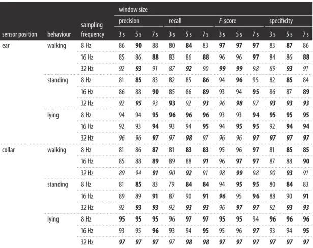
In table 7, a summary of the precision, recall,F-score and specificity is presented. The classification
performance for this activity provided the lowest performance values with 80% recall on a 3 s window and 8 Hz sampling frequency for ear and 81% for collar data. Overall, the classification performance for this activity also showed the greatest range of variation with values ranging between 80% (recall) and
99% (specificity) for both ear and 81% (recall) and 99% (specificity) for collar data. Values ofF-score varied
between 83% and 93% for ear data and between 81% and 93% for collar data. The bestF-score value (93%)
10
rsos
.ro
yalsociet
ypublishing
.or
g
R.
Soc
.open
sc
i.
5
:1
71442
...
Table 7.Performance metrics of the classification algorithm. Summary of the precision, recall,F-score and specificity metrics for sheep
activity classification using both the ear-mounted and collar-mounted sensors with window sizes of 3, 5 and 7 s with sampling frequencies of 8, 16 and 32 Hz. In bold are the highest values for precision, recall,F-score and specificity when comparing across window sizes. In italics are the highest values for precision, recall,F-score and specificity when comparing only across different sample frequencies.
window size
precision recall F-score specificity
sensor position behaviour
sampling
frequency 3 s 5 s 7 s 3 s 5 s 7 s 3 s 5 s 7 s 3 s 5 s 7 s
ear walking 8 Hz 86 90 88 80 84 83 97 97 97 83 87 86
. . . .
16 Hz 85 86 88 83 86 88 96 96 97 84 86 88
. . . .
32 Hz 92 93 91 87 92 90 99 99 98 89 93 91
. . . .
standing 8 Hz 81 85 83 82 85 86 94 96 95 82 85 84
. . . .
16 Hz 86 88 90 85 86 89 93 94 95 86 87 89
. . . .
32 Hz 92 95 93 93 92 93 96 98 97 93 93 93
. . . .
lying 8 Hz 94 94 95 96 96 96 93 93 94 95 95 95
. . . .
16 Hz 92 93 94 93 94 95 94 95 95 92 94 94
. . . .
32 Hz 96 96 97 97 98 97 96 96 97 97 97 97
. . . .
collar walking 8 Hz 81 86 87 81 83 83 95 96 97 81 85 85
. . . .
16 Hz 85 88 89 89 88 91 96 97 97 87 88 90
. . . .
32 Hz 89 94 91 90 92 91 98 99 98 90 93 91
. . . .
standing 8 Hz 81 85 83 79 84 84 94 95 95 80 84 83
. . . .
16 Hz 89 89 91 87 90 91 96 95 96 88 90 91
. . . .
32 Hz 92 93 93 92 93 93 96 97 97 92 93 93
. . . .
lying 8 Hz 95 95 95 96 97 97 95 95 94 96 96 96
. . . .
16 Hz 93 95 96 93 94 95 95 96 97 93 94 95
. . . .
32 Hz 97 97 97 97 98 98 97 97 97 97 97 97
. . . .
classification of walking (precision of 88.77%, recall, 87.77%, on average for ear; and precision of 87.77% and recall of 87.55% on average for collar).
3.2.2. Standing
The classification performance for this activity was very similar to walking as performance values ranged between 81% and 98% for ear data and 80% and 97% for collar data. Values for the precision, recall and
F-score varied between 81% and 95% in ear data and between 80% and 93% in collar data. Similarly to
walking, the highest performance values were obtained for specificity, with values ranging between 93% and 98% for ear data and 94% to 97% for collar data. For the standing behaviour, precision and recall values were above or very close to 90% for 16 and 32 Hz sample frequencies, and between 81% and 85% for 8 Hz data in both ear and collar data. The classification performance of standing for the ear data (precision of 88.11% and recall of 87.88%, on average) was similar to the collar data (precision of 88.44% and recall of 88.11%, on average).
3.2.3. Lying
For this activity, the best performance results were obtained with values above 93% for precision, recall,
F-score and specificity in collar data. Additionally, all the performance metrics for the lying behaviour
11
rsos
.ro
yalsociet
ypublishing
.or
g
R.
Soc
.open
sc
i.
5
:1
71442
...
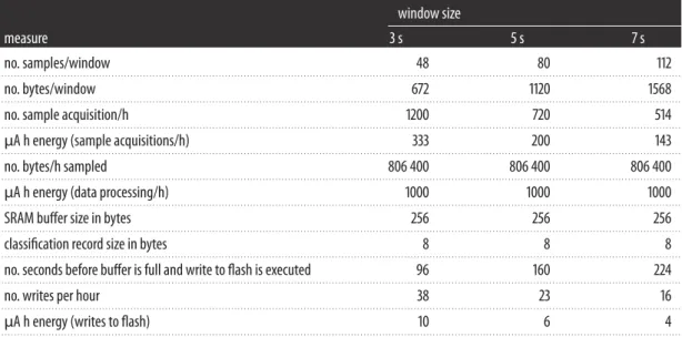
Table 8.Energy consumption for data acquisition during classification and written to flash. Measurements of energy are express inµA h
(microampere hour). Measurements were provided by Intel®.
window size
measure 3 s 5 s 7 s
no. samples/window 48 80 112
. . . .
no. bytes/window 672 1120 1568
. . . .
no. sample acquisition/h 1200 720 514
. . . .
µA h energy (sample acquisitions/h) 333 200 143
. . . .
no. bytes/h sampled 806 400 806 400 806 400
. . . .
µA h energy (data processing/h) 1000 1000 1000
. . . .
SRAM buffer size in bytes 256 256 256
. . . .
classification record size in bytes 8 8 8
. . . .
no. seconds before buffer is full and write to flash is executed 96 160 224
. . . .
no. writes per hour 38 23 16
. . . .
µA h energy (writes to flash) 10 6 4
. . . .
of 98% was obtained for 32 Hz data and 5 and 7 s windows using collar data, and a 98% maximum recall for 32 Hz, and 5 s window size for ear data. Of the three different behaviours, lying was the one with the highest overall performance for all the different window sizes and sampling frequencies.
The classification performance for the standing and walking behaviours improved when increasing sampling frequency and window size. Specificity values were in general very high (above 90%) for the different behaviours at all sampling frequencies and window sizes. The highest specificity values were obtained for the walking behaviour (overall average of 97.16%) compared with specificity values of the standing behaviour (overall average of 95.33%) and the lying behaviour (overall average of 95.33%). Specificity values were very similar in ear and collar data; with average values of 97.33%, 95.33% and 94.77% for walking, standing and lying in ear data, and 97%, 95.66% and 95.88% in collar data.
Overall, the best results for ear data are observed when using the 32 Hz sample frequency dataset and 7 s windows, giving an average precision across the three behaviours of 93.66% and an average recall of 93.33%. The best performances for collar sensor data were observed when using the 32 Hz sample frequency and 7 s windows, with an average precision of 93.66% and an average recall of 94% across the three behaviours. Moreover, when comparing between 3 and 5 s window sizes, there is an average
increase of 1.5% in accuracy, 2% in precision, 1.77% in recall, 0.61% inF-score and 1.77% in specificity.
When comparing between 5 and 7 s window sizes, we obtained an average increase of 0.33% in accuracy,
0.444% in recall, 0.111% inF-score and 0.056% in specificity and an average 0.056% decrease in precision.
There is an average increase of 1.53% on the performance between 3 and 5 s window sizes and an average increase of 0.177% between 5 and 7 s window sizes. The relative difference in performance between 3 and 7 s windows was larger than between 5 and 7 s.
3.3. Energy consumption
There were energy consumption benefits for using a 7 s window compared with a 5 or 3 s window, as
shown intable 8. Energy consumption benefits included: a reduction of the number of samples acquired
for the classification (1200, 720, and 514 for 3, 5 and 7 s, respectively), a reduction of the energy required to acquire the samples (333, 200 and 143 µA h for 3, 5 and 7 s, respectively), and increase of the time before buffer was full to write to flash (96, 160 and 224 s for 3, 5 and 7 s, respectively), a decrease of the number writes per hour (38, 23 and 16 for 3, 5 and 7 s, respectively), and a decrease of the energy used to write to flash (10, 6 and 4 µA h for 3, 5 and 7 s, respectively).
4. Discussion
12
rsos
.ro
yalsociet
ypublishing
.or
g
R.
Soc
.open
sc
i.
5
:1
71442
...
classification models trained on collar sensor data showed very similar results to models trained on ear
data when classifying walking, standing and lying in sheep, with an average difference of±0.44% in
accuracy, in±0.11% in precision and±0.74% in recall when comparing across all sampling frequencies
and window sizes that were used in this study. A previous study [14] has also shown differences in
the performance of a classifier when using sensors in different positions on the body of an animal. The small differences in performance between the collar-mounted sensor and the ear-mounted sensor in our study could be due to the relatively higher noise in the ear data, which results from the greater freedom of movement of the sensor attached to the ear and other behaviours, such as head shaking. In comparison with the neck collar, the advantage of an ear-mounted sensor is that it could potentially be integrated into the current ear tag identifier, providing richer functionality in only one sensor. Whilst the differences between ear and collar position in the current study might be negligible for the classification of behaviours such as standing, walking and lying, the differences could be substantial for other behaviours such as head nodding and grazing/browsing where the accelerometer is likely to register much more weaker-amplitude movements when mounted on the neck. However, this needs to be further investigated.
When comparing across different window sizes, the performance of the random forest algorithm suggests that overall the 7 s window is the best for classifying the sheep behaviours of walking, standing
and lying, as in general the accuracy, precision, recall, F-score and specificity of the classification
increased with increasing window sizes for both ear- and collar-mounted sensors. A recent study on
classification of sheep behaviour by Alvarengaet al. [18] reported an increase from 82.9% to 83.5% on
classification accuracy for activities such as grazing, lying, running, standing and walking when using a 5 s window compared with a 3 s window and a slight decrease to 83.4% when using a 10 s window. When a 14 s window was tried in the current study (results not shown), a significant drop in accuracy was observed (i.e. drop of accuracy to 84% for ear data and 93% for collar data at 32 Hz). The choice of window size depends on the activity to be classified; shorter windows are generally considered better, as they are
less likely to have variability or transition in behaviour [20]. At the same time, longer windows tend to be
better for more complex behaviours as they are more likely to contain more information and thus result
in better classification accuracy [19,20]. Interestingly, in this study the shortest window size (3 s) showed
the worst performance for walking and standing behaviours. However, classification performance for lying did not vary much between 3 and 7 s, perhaps due to lying being a comparatively less complex behaviour, thus needing less information for accurate classification. Overall, 7 s window size was also most energy efficient despite the difference in algorithm performance between 7 and 5 s being small. Hence, the trade-off between classification performance and energy consumption is important in the choice of a window size for implementation purposes.
When comparing across the different sampling frequencies for both ear and collar data, there was a general increase in all the performance measures for the sampling frequencies of 16 and 32 Hz. The difference in accuracy between 16 and 32 Hz was small (5% for ear data and 3.33% for collar data, on average). However, increasing the sampling frequency from 16 to 32 Hz can reduce the battery life by up
to a half [26]. In other words, an increase up to 5% in classification performance may come at the cost of
reducing battery life by up to half. Therefore, the selection of the sampling frequency has to be carefully considered in the configuration of an automated monitoring system as it has a large impact on energy,
transmission bandwidth and storage capacity requirements [26].
The classification algorithm in the current study was highly accurate and precise for each of the
behaviours as illustrated in tables5and7. The performance results scored much higher than previously
reported by other studies on sheep for similar behaviours (e.g. 85.5% accuracy [18] and 87.1% to 89.7%
overall accuracy [16]). This could be because in the current study we used features extracted from both
accelerometer and gyroscope data for classification unlike previous studies. Lying was the behaviour with the highest precision (95.05% average) and recall (95.94% average) for both ear and collar data when comparing with walking (precision 88.27% and recall 86.72%) and standing (precision 87.94% and recall 88%). Lying can be more easily classified as sheep move significantly less than when standing and walking. The highest misclassification was observed between walking and standing (see confusion matrices in the electronic supplementary material). This is probably due to the grazing activity (which is most likely to occur when sheep are standing) causing accelerations similar to walking, leading to misclassifications. In the current study, grazing activity was not separately recorded and further work is needed to investigate grazing and non-grazing activities.
13
rsos
.ro
yalsociet
ypublishing
.or
g
R.
Soc
.open
sc
i.
5
:1
71442
...
costs. Previous studies have used complex methods such as hidden Markov models (HMM) [13], support
vector machines (SVM) [11] and generalized mixed linear models (GMLM) [12] or simple methods
such as decision trees [13] for the classification of behaviours in farm animals. HMM, SVM and GMLM
can have high computational cost and hence they are typically less appealing for automated, real-time monitoring devices. Decision trees can offer a low computational cost; however, they tend to overfit the
data [2]. Random forest algorithms can improve the overfitting problem of decision trees algorithms
while maintaining a relatively low computational cost [2]. Hence, random forest represents a potentially
good candidate for embedding in sensors mounted on animals. Additionally, the results obtained in this study show that a random forest classifier can accurately classify different relevant behaviours in sheep with a very high accuracy.
While in the study we have evaluated different window sizes and sampling frequencies that are suited for the real-time monitoring of behaviour classification of sheep; we need to validate our results in a field trial. In addition, we did not evaluate feature importance and further selection which will be important in terms of computational cost for real-time monitoring.
5. Conclusion
The results from this study show that biologically relevant behaviours in sheep such as walking, standing and lying, can be accurately classified (89–95%), using a random forest classifier and extract specific feature characteristics that consider window size, position and sampling frequency. Evaluation of window sizes suggests 7 s to be the best window size for achieving high classification accuracy of walking, standing and lying and also with respect to energy performance. The highest performance of the classifier was obtained when using a sampling frequency of 32 Hz. However, results using a 16 Hz sample frequency were comparable, thus suggesting significant benefits of using 16 Hz for real-time monitoring. Overall, the level of agreement of the accuracy of the classification between collar and ear data was high (0.84–0.911), except at 8 Hz and 3 s. However, ear-mounted sensors could be more easily integrated into the already existing ear tag identifiers for sheep.
Ethics. The study was reviewed and approved by the School of Veterinary Medicine and Science Ethics and Welfare Committee under the unique number 1481 150603.
Data accessibility. All data files, can be found at Dryad:http://dx.doi.org/10.5061/dryad.h5c80[42].
Authors’ contributions. J.K. and K.E. conceived the study and secured funding; J.K. and E.W. designed the study; E.W., J.Y. and J.K. collected the data; E.W., J.Y., J.M., T.D. and A.W. participated in in data curation and data visualization; C.C. and J.M. did software programming and coding; K.E. did programming of the hardware and provided the materials for data collection; C.C., J.M., J.V. and J.K. did data analysis data analysis and data validation. E.W., J.M., J.V. and J.K. drafted the initial manuscript. All authors reviewed and edited the manuscript and gave approval of the publication.
Competing interests. The authors declare that they do not have competing interests.
Funding. Funded by grant from Innovate UK (132164) and BBSRC grant no. BB/N014235/1.
Acknowledgements. We would like to thank Dr Peers Davies, Nikki Bollard and Emma Gurney for their help with field trial.
References
1. McGowan Jet al.2016 Integrating research using animal-borne telemetry with the needs of conservation management.J. Appl. Ecol.54, 423–429. (doi:10.1111/1365-2664.12755) 2. Valleta JJ, Torney C, Kings M, Thornton A, Madden J.
2017 Applications of machine learning in animal behaviour studies.Anim. Behav.124, 203–220. (doi:10.1016/j.anbehav.2016.12.005) 3. Neethirajan S. 2017 Recent advances in wearable
sensors for animal health management.Sens. Bio Sens. Res.12, 15–29. (doi:10.1016/j.sbsr.2016. 11.004)
4. Jukan A, Masip-Bruin X, Amla N. 2017 Smart computing and sensing technologies for animal welfare: a systematic review.ACM Comput. Surveys
50, Article No. 10. (doi:10.1145/3041960) 5. Molony V, Kent JE. 1997 Assessment of acute pain in
farm animals using behavioural and physiological
measurements.J. Anim. Sci.75, 266–272. (doi:10.2527/1997.751266x)
6. Fitzpatric J, Scott M, Nolan A. 2006 Assessment of pain and welfare on sheep.Small Ruminant Res.62, 55–61. (doi:10.1016/j.smallrumres.2005.07.028) 7. Ley SJ, Livingston A, Waterman AE. 1989 The effect
of chronic clinical pain on thermal mechanical thresholds in sheep.Pain39, 353–357. (doi:10.1016/ 0304-3959(89)90049-3)
8. Kaler J, Wassink GJ, Green LE. 2009 The inter- and intra-observer reliability of locomotion scoring scale for sheep.Vet. J.180, 189–194. (doi:10.1016/ j.tvjl.2007.12.028)
9. Miedema, JM. 2010 Investigating the use of behavioural, accelerometer and heart rate measurements to predict calving in dairy cows. PhD thesis, Royal (Dick) School of Veterinary Studies, The University of Edinburgh.
10. Gerencsér L, Vásárhelyi G, Nagy M, Vicsek T, Miklósi A. 2013 Identification of behaviour in freely moving dogs (Canis familiaris) using inertial sensors.PLoS ONE8, e0077814. (doi:10.1371/journal.pone. 0077814)
11. Martiskainen P, Järvinen M, Skön JP, Tiirikainen J, Kolehmainen M, Mononen J. 2009 Cow behaviour pattern recognition using a three-dimensional accelerometer and support vector machines.Appl. Anim. Behav. Sci.119, 32–38.
(doi:10.1016/j.applanim.2009.03.005) 12. Robert B, White BJ, Renter DG, Larson RL. 2009
Evaluation of three-dimensional accelerometers to monitor and classify behaviour patterns in cattle.
Comput. Electron. Agric.67, 80–84. (doi:1016/ j.compag.2009.03.002)
14
rsos
.ro
yalsociet
ypublishing
.or
g
R.
Soc
.open
sc
i.
5
:1
71442
...of behaviour in housed dairy cows using an accelerometer-based activity monitoring system.
Anim. Biotelem.3, 15. (doi:1186/s40317-015-0045-8) 14. Moreau M, Siebert S, Buerkert A, Schlecht E. 2009
Using of a tri-axial accelerometer for automated recording and classification of goats’ grazing behaviour.Appl. Anim. Behav. Sci.199, 158–170. (doi:1016/j.applanim.2009.04.008)
15. Marchioroa GF, Cornou C, Kristensen AR, Madsen J. 2011 Sows’ activity classification device using acceleration data – a resource constrained approach.Comput. Electron Agr.77, 110–117. (doi:1016/j.compag.2011.04.004)
16. Marais J, Le Roux SP, Wolhuter R, Niesler T. 2014 Automatic classification of sheep behaviour using 3-axis accelerometer data. InProc. 25th Annual Symp. Pattern Recognition Association of South Africa
(PRASA),Cape Town, South Africa, 27–28 November, pp. 97–102.
17. Radeski M, Ilieski V. 2016 Gait and posture discrimination in sheep using a tri-axial accelerometer.Animal11, 1249–1257. (doi:10.1017/ S175173111600255X)
18. Alvarenga FAP, Borges I, Palković RJ, Oddy VH, Dobos RC. 2016 Using a three-axis accelerometer to identify and classify sheep behaviour at pasture.
Appl. Anim. Behav. Sci.181, 91–99. (doi:10.1016/ j.applanim.2016.05.026)
19. Bersch SD, Azzi D, Khusainov R, Achumba IW, Ries J. 2014 Sensor data acquisition and processing parameter for human activity classification.Sensors
14, 4239–4270. (doi:10.3390/s140304239) 20. Banos O, Galvez J-M, Damas M, Pomares H, Rojas I.
2014 Window size impact in human activity recognition.Sensors14, 6474–6499. (doi:10.3390/ s140406474)
21. Gao L, Bourke AK, Nelson J. 2014 Evaluation of accelerometer based multi-sensor versus single-sensor activity recognition systems.Med. Eng. Phys.36, 779–785. (doi:10.1016/j.medengphy. 2014.02.012)
22. Attal F, Mohammed S, Dedabrishvii M, Chamroukhi F, Oukhellou L, Amirat Y. 2015 Physical human activity recognition using wearable sensors.Sensors
15, 31 314–31 338. (doi:10.3390/s151229858) 23. Ohja T, Misra S, Raghuwanshi NS. 2015 Wireless
sensor network for agriculture: the state-of-the-art in practice and future challenges.Comput. Electron. Agr118, 66–84. (doi:10.1016/j.compag.2015. 08.011)
24. Russel A. 1984 Body condition scoring of sheep.
Practice6, 91–93. (doi:10.1136/inpract.6.3.91) 25. Agriculture and Horticulture Development Board
(AHDB). 2017. Seehttps://beefandlamb.ahdb.org. uk/wp-content/uploads/2013/06/brp_l_Sheep_ BCS_190713.pdf.
26. Khan A, Hammerla N, Mellor S, Plötz T. 2016 Optimising sampling rates for accelerometer-based human activity.Pattern Recogn. Lett.73, 33–40. (doi:10.1016/j.patrec.2016.01.001)
27. Python Software Foundation. 2010Python Language Reference, version 2.7. Seehttp://www.python.org. 28. Qasem L, Cardew A, Wilson A, Griffiths I, Halsey LG,
Shepard ELC, Gleiss AC, Wilson R. 2012 Tri-axial dynamic acceleration as a proxy for animal energy expenditure; should we be summing values or calculating the vector?PLoS ONE7, e31187. (doi:10.1371/journal.pone.0031187) 29. Figo D, Diniz PC, Ferreira DR, Cardoso JM. 2010
Preprocessing techniques for context recognition from accelerometer data.Pers. Ubiquit. Comput.14, 645–662. (doi:10.1007/s00779-010-0293-9) 30. Piercee SJ, Goulermas JY, Kenney PJ, Howard D.
2009 A comparison of feature extraction methods for classification of dynamic activities from accelerometer data.IEEE. T. Bio. Med. Eng.56, 871–879. (doi:10.1109/TBME.2008.2006190) 31. Wundersitz DW, Josman C, Gupta R, Netto KJ,
Gastin PB, Robertson S. 2015 Classification of team sport activities using a single wearable tracking device.J. Biomech.48, 3975–3981. (doi:10.1016/ j.biomech.2015.09.015)
32. Bao L, Intille SS. 2004 Activity recognition from user-annotated acceleration data. InInter. Conf. Pervasive Comput., Linz and Vienna, Austria, 21–23 April, pp. 1–17. Berlin, Germany: Springer. 33. Breiman L. 2001 Random forests.Mach. Learn.45,
5–32. (doi:10.1023/A:10109334)
34. Cutler DR, Edwards TC, Beard KH, Cutler A, Hess KT, Gibson J, Lawler JJ. 2007 Random forest for classification in ecology.Ecology88, 2783–2792. (doi:10.1890/07-0539.1)
35. Hastie T, Tibshirani R, Friedman J. 2008The elements of statistical learning, 2nd edn. Berlin, Germany: Springer.
36. Fontama V, Barga R, Tok WH. 2015Predictive analytics with Microsoft Azure machine learning: build and deploy actionable solutions in minutes. Berkeley, CA: Apress.
37. Browne MW. 2000 Cross-validation methods.
J. Math. Psychol.44, 108–132. (doi:10.1006/jmps. 1999.1279)
38. Burman P. 1989 A comparative study of ordinary cross-validation, v-fold cross-validation and the repeated learning-testing methods.Biometrika76, 503–514. (doi:10.2307/2336116)
39. Mitchell E, Monaghan D, O’Connor NE. 2013 Classification of sporting activities using smartphone accelerometers.Sensors13, 5317–5337. (doi:10.3390/s130405317)
40. Ben-David A. 2008 Comparison of classification accuracy using Cohen’s weighted kappa.Expert Syst. Appl.34, 825–832. (doi:10.1016/j.eswa.2006.10.022) 41. R Core Team. 2013R: A language and environment for statistical computing. Vienna, Austria: R Foundation for Statistical Computing. See https://www.R-project.org/.