The use of PSD analysis on BeiDou and GPS 10Hz dynamic data for change detection

(1)

Elsevier Editorial System(tm) for Advances in Space Research

Manuscript Draft

Manuscript Number: ASR-D-16-00028R3

Title: The use of PSD Analysis on BeiDou and GPS 10Hz Dynamic data for change detection

Article Type: SI: High-rate GNSS

Keywords: GPS; BeiDou; Kinematic

Corresponding Author: Professor. Gethin Wyn Roberts, PhD, BEng

Corresponding Author's Institution: The University of Nottingham Ningbo China

First Author: Gethin Wyn Roberts, PhD, BEng

Order of Authors: Gethin Wyn Roberts, PhD, BEng; Xu Tang, BSc PhD

Abstract: This paper examines the use of GPS and BeiDou data to measure the movements of two oscillating platforms in a series of field

experiments. Data were gathered from a variety of GNSS receivers at a rate of 10Hz, and processed in an on the fly manner, resulting in 3D coordinates at a 10Hz rate with the corresponding precise time. These data were then analysed using a Power Spectral Density (PSD) function to derive the frequency of the movements. The positional data were also compared by matching a 500 epoch section of the data from the start with 190 successive 500 epoch long sections in order to demonstrate whether the movement measured was constant throughout, or whether there were any changes. The results show that the correlation of the positional data over a 30,737 epoch period deviates between 99.8% to 76.7% correlation with RMS values of 89.2%, 87.9% and 77.5% in the Eastings, Northings and Vertical directions respectively when using GPS. The RMS of the Eastings and Northings remain the same when BeiDou is introduced, but the height component improves slightly to 78.9%. The frequency analysis of the same 500 epoch long sections is constantly measured at 0.1172Hz in all three positional components, illustrating less deviation when analysing the frequencies. The main conclusion is that analysis of the resulting PSD output from GNSS data gathered on an oscillating platform is more

constant and precise than analysing the results of the coordinates alone. This suggests that such analysis would be well suited for a Structural Health Monitoring system. The introduction of BeiDou also improves the results slightly, even in its current incomplete constellation. The novelty of this work is the analysis of the movements in such a

(2)

(3)

1 2 3 4 5 6 7 8 9 10 11 12 13 14 15 16 17 18 19 20 21 22 23 24 25 26 27 28 29 30 31 32 33 34 35 36 37 38 39 40 41 42 43 44 45 46 47 48 49 50 51 52 53 54 55 56 57 58 59 60 61

The use of PSD Analysis on BeiDou and GPS 10Hz Dynamic data for change detection

Prof Gethin Wyn Roberts, Xu Tang

[email protected], [email protected]

The University of Nottingham Ningbo, China

199 Taikang Road East

Ningbo, 315100

China.

1. Abstract

This paper examines the use of GPS and BeiDou data to measure the movements of two oscillating platforms in a series of field experiments. Data were gathered from a variety of GNSS receivers at a rate of 10Hz, and processed in an on the fly manner, resulting in 3D coordinates at a 10Hz rate with the corresponding precise time. These data were then analysed using a Power Spectral Density (PSD) function to derive the frequency of the movements. The positional data were also compared by matching a 500 epoch section of the data from the start with 190 successive 500 epoch long sections in order to demonstrate whether the movement measured was constant throughout, or whether there were any changes. The results show that the correlation of the positional data over a 30,737 epoch period deviates between 99.8% to 76.7% correlation with RMS values of 89.2%, 87.9% and 77.5% in the Eastings, Northings and Vertical directions respectively when using GPS. The RMS of the Eastings and Northings remain the same when BeiDou is introduced, but the height component improves slightly to 78.9%. The frequency analysis of the same 500 epoch long sections is constantly measured at 0.1172Hz in all three positional components, illustrating less deviation when analysing the frequencies. The main conclusion is that analysis of the resulting PSD output from GNSS data gathered on an oscillating platform is more constant and precise than analysing the results of the coordinates alone. This suggests that such analysis would be well suited for a Structural Health Monitoring system. The introduction of BeiDou also improves the results slightly, even in its current incomplete constellation. The novelty of this work is the analysis of the movements in such a controlled environment, and the correlation approach of the resulting positional output as well as the frequency derivation from the positions using both GPS and BeiDou.

2. Introduction

The use of Global Navigation Satellite Systems (GNSS) for deflection monitoring of structures (Rizos et al., 2010, Çelebi, 1998, Teague et al., 1995, Lovse et al, 1995), and in particular long span bridges (Roberts et al., 2014) has been an area of ongoing research for over 20 years. The work initially focussed on using carrier phase Global Positioning System (GPS) observations, gathered from a reference GPS receiver located adjacent to the bridge, as well as one or more GPS receivers attached to the bridge. Typically, on the handrail at deck level or on top of the support towers. The bridge data was initially gathered at a 1Hz rate, but over successive pieces of work, this soon increased to 10Hz, 20Hz and even 100Hz in some instances. The data were processed in an on the fly manner (Hofmann-Wellenhof

Manuscript

(4)

1 2 3 4 5 6 7 8 9 10 11 12 13 14 15 16 17 18 19 20 21 22 23 24 25 26 27 28 29 30 31 32 33 34 35 36 37 38 39 40 41 42 43 44 45 46 47 48 49 50 51 52 53 54 55 56 57 58 59 60

et al., 2008) relative to the reference receiver data, either in a post processed or real time manner. Movements at decimetre level on long span bridges were calculated, as well as synchronised movements between multiple GPS receivers located on a bridge (Roberts et al., 2014). More recently, combined GNSS data have been used to determine the movements, including data gathered directly on the suspension cables (Roberts et al., 2014).

GNSS data gathered using survey grade receivers typically consist of pseudorange and carrier phase data, on one, two or even three frequencies. Such data can be gathered at 10Hz, 20Hz or even 100Hz when using specific GNSS receivers. These data can also consist of GPS, GLONASS, BDS (BeiDou System), Galileo and even Regional Navigation Satellite Systems (RNSS) such as the Japanese Quazi Zenith Satellite System (QZSS). This all depends on the specific GNSS receiver used. The resolution of the carrier phase measurement is of the order of sub-millimetre (Roberts et al., 2012).

Due to the GNSS data consisting of a precise time with the corresponding range related data; the frequency of the movements can also be derived (Psimoulis and Stiros, 2008; Psimoulis et al., 2008, Ogundipe et al., 2014, Çelebi et al., 1999, Roberts et al., 2012). Such movements have been used to detect the vibration frequencies of tall buildings (Xu and Wu, 2014). The use of frequency analysis using Fast Fourier Transformations (FFT) and Power Spectral Density (PSD) analysis looks like a promising method to analyse the data, and also to detect changes in the characteristics of the movements, and hence to possibly use such frequency analysis as part of a Structural Health Monitoring (SHM) scheme. Such a SHM could be created using GNSS data from a bridge or structure to create and validate a realistic structural analyses model, such as a Finite Element Model (FEM). Periodically, more GNSS data gathered from the structure could be used to continuously compare the real data (GNSS) with the model in order to look at the deviations. GNSS data have been shown again and again to be very precise. Xu et al. (2013) illustrate that it is possible to obtain accuracies of the order of 2-4mm in plan and vertical accuracies at the sub-centimetre level when using Precise Point Positioning. Other work have shown that precise millimetre level positioning is possible (Chen et al. 2015, Vaclavoic and Dousa, 2015). BDS is currently under development, but already has good satellite coverage over China and the surrounding area, due to the addition of Geostationary Earth Orbit (GEO) and Inclined Geosynchronous Orbit (IGSO), in addition to the Mid Earth Orbit (MEO) satellites, and constantly improving (Jin, 2013, Xiao et al., 2016). Various pieces of research have been undertaken, including combining GPS and BDS signals for better ambiguity resolution and positioning. Specific research, for example, has been carried out on improving attitude determination through integrating GPS and BDS (Nadarajah et al., 2014), and improving ambiguity resolution for Low Earth Orbiting satellite formation flying (Verhagen and Teunissen, 2014). Research has also been ongoing, integrating GPS and GNSS with accelerometers (Roberts et al., 2004) as well as rapidly developing MEMS based accelerometers (Tu et al., 2013, Tu et al., 2014). Such integration can result in a complimentary system, where the advantages of GPS/GNSS and the accelerometers are combined. Such advantages include the rapid data available from the accelerometers, the lack of drift in the GNSS data and the higher precision of the MEMS sensors.

(5)

1 2 3 4 5 6 7 8 9 10 11 12 13 14 15 16 17 18 19 20 21 22 23 24 25 26 27 28 29 30 31 32 33 34 35 36 37 38 39 40 41 42 43 44 45 46 47 48 49 50 51 52 53 54 55 56 57 58 59 60 61

located at the end. Both experiments included the use of multi-GNSS receivers connected to the same antenna using a cable splitter. These data were then post processed relative to the GNSS receivers attached to the reference station pillar. All the experiments were carried out on the roof of the Science and Engineering Building (SEB) at the University of Nottingham Ningbo China (UNNC) campus.

This paper concentrates on data from specific receivers, and also through analysing the BDS and GPS data processing, either as individual solutions or as a combined multi-GNSS solution. The analysis of the results using PSD and the correlation function attempts to illustrate that analysis of the frequency of the oscillating data derived from GNSS, and any changes in the frequency, is a strong method to compare any changes in the movement characteristics of the structure. Indeed, this technique can also be used to validate that there have been no changes in the movement characteristics of a structure. Such changes could be due to damage or degradation of the structure, or changes in the wind loading, traffic loading or temperature changes. Changes in the movement characteristics would be expected to correlate to these external factors, and any discrepancy could also suggest that damage has occurred (Psimoulis and Stiros, 2008, Psimoulis et al., 2008).

3. Field Tests

This section details the field trials carried out in order to gather the data used for analysis in section 4. Two sets of field trials were conducted on two different platforms in order to analyse and assess the performance of 10 Hz GNSS data, consisting of GPS and BDS, processed as GPS only, BDS only and a combined GPS/BDS solution. The platforms consist of a bungee cord based rig; which moved predominately in the vertical direction, and a rotating arm rig; which moves in a horizontal circular manner also with smaller changes in the vertical displacements. Both field trials were carried out on the roof of the SEB at UNNC, which is a reasonably open sky environment. These two types of experiments were conducted in order to simulate real movements on a dynamic structure, such as a long span bridge, but in a controlled manner. The bungee experiment was ideal for such simulation, apart from the fact that it required constant excitation. The rotating rig provided a platform that was able to move with a very constant and precise motion, shown later in the results. Such controlled environments mean that there are less external uncertainties in the results and that the frequencies and movements occurring are more constant and stable than when gathering data from, for example, a long span bridge. The following two sub-sections detail the two field tests.

a. Bungee Experiment

(6)

1 2 3 4 5 6 7 8 9 10 11 12 13 14 15 16 17 18 19 20 21 22 23 24 25 26 27 28 29 30 31 32 33 34 35 36 37 38 39 40 41 42 43 44 45 46 47 48 49 50 51 52 53 54 55 56 57 58 59 60

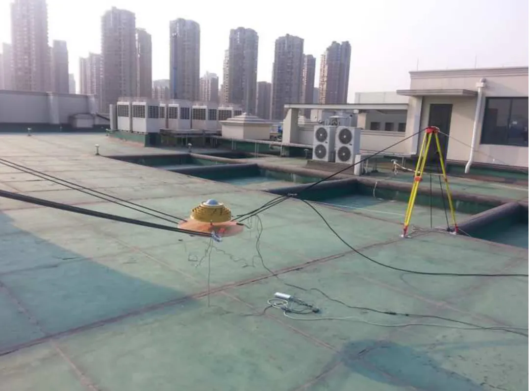
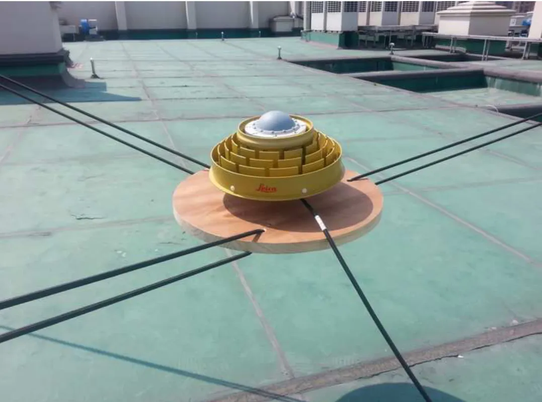
Figure 1, The Bungee Experiment located on the roof of the Science and Engineering Building, UNNC (left), and a close up view of the Leica AR25 choke ring GNSS antenna (right).

This experiment attempts to simulate, in a controlled manner, deflections similar to the ones of long span suspension bridges. Typically, large bridges have periods of movements of a few seconds, even up to 10s of seconds, resulting in frequencies as low as 0.1Hz (Roberts et al, 2014). The Forth Road Bridge, The Humber Bridge, The Severn Suspension Bridge have main vertical frequencies of 0.1055Hz, 0.116Hz and 0.1040Hz respectively (Roberts et al, 2014: Roberts et al., 2012), determined using GPS.

The bungee platform was excited by pulling it down by hand and letting it go, and then periodically exciting it by hand. The platform would then move with its own natural frequency, gradually decreasing in amplitude unless excited again either by hand or by any wind. This was carried out over a 2 hour period. There were also instances when the platform was kept static, and even placed upon a tripod in order to look at the characteristics of the GNSS noise.

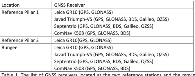
A variety of GNSS receivers were attached to the reference pillars, as well as the test rig. Multiple GNSS receivers were connected to the test rig and the main reference pillar using a GEMS antenna splitter. Table 1 illustrates the GNSS receiver layout, as well as the GNSS constellations that each receiver is capable to track and record.

Location GNSS Receiver

Reference Pillar 1 Leica GR10 (GPS, GLONASS)

Javad Triumph-VS (GPS, GLONASS, BDS, Galileo, QZSS)

Septentrio (GPS, GLONASS, BDS, Galileo, QZSS)

ComNav K508 (GPS, GLONASS, BDS)

Reference Pillar 2 Leica GR10(GPS, GLONASS)

Bungee Leica GR10 (GPS, GLONASS)

Table 1, The list of GNSS receivers located at the two reference stations and the moving bungee platform.

All the GNSS receivers gathered carrier phase and pseudorange GNSS data at a rate of 10Hz throughout the experiment. All the receivers are capable of gathering triple frequency GPS and Galileo data, and the ComNav receiver is in addition able to gather BDS triple frequency data. This paper presents data derived by processing dual frequency GPS and BDS data.

(7)

1 2 3 4 5 6 7 8 9 10 11 12 13 14 15 16 17 18 19 20 21 22 23 24 25 26 27 28 29 30 31 32 33 34 35 36 37 38 39 40 41 42 43 44 45 46 47 48 49 50 51 52 53 54 55 56 57 58 59 60 61

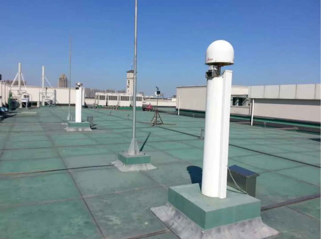
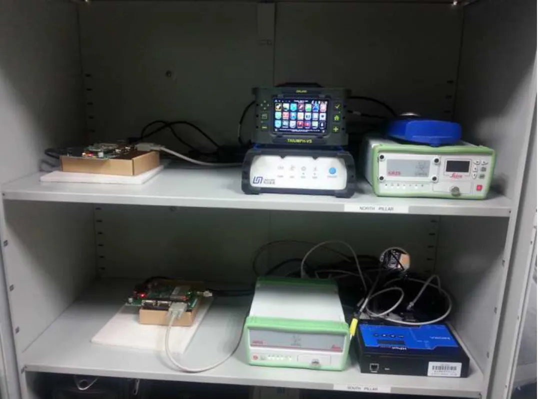
Figure 2, The GNSS pillars located on top of the UNNC Science and Engineering Building (left), and the GNSS receivers located in the GNSS laboratory (right)

Data were gathered over a 2-hour period, and the Leica and ComNav data are used in this paper.

b. Rotating Arm Experiment

The second experiment consisted of using the rotating arm rig, fabricated at UNNC. This consists of an electric motor, attached to a 3m long arm, whereby a GNSS antenna can be attached to one end, counterbalanced with a weight on the other, Figure 3. The GNSS receivers are located inside the box that sits on top of the rig, which also rotates around with the rig. This prevents the antenna cable from being tangled. All the GNSS receivers require to be battery operated when using this rig. During this experiment, Leica GR10 and Javad Triumph-VS receivers were attached to both the main reference pillar1 and the rotating arm. In fact, two Leica GNSS receivers were attached to each of the reference pillar and rotating arm, through using antenna cable splitters. This will allow further analysis of the errors through using the zero baseline at the reference station as well as a zero baseline at the rotating arm.

The electric motor on the rig was initially set up to rotate with a period of approximately 9 seconds. The movements are mainly in the horizontal directions (East and North), but there are also reduced vertical movements, mainly due to the rig not being perfectly horizontal. A Leica AR25 choke ring antenna was used on the rig, and all the data were gathered at 10Hz. The distance between the reference1 pillar and the centre of the rotating rig is of the order of 35.942m.

Figure 3, The rotating arm rig located on the roof of the Science and Engineering building. The GNSS receivers are located within the rotating box, and the GNSS antenna located at the end of the arm.

(8)

1 2 3 4 5 6 7 8 9 10 11 12 13 14 15 16 17 18 19 20 21 22 23 24 25 26 27 28 29 30 31 32 33 34 35 36 37 38 39 40 41 42 43 44 45 46 47 48 49 50 51 52 53 54 55 56 57 58 59 60

4. Results and Analysis

This section illustrates the results of the two experiments, and uses PSD analysis to calculate the dominant frequencies of the oscillating movements, as well as using a correlation function to compare the repetition of the data with itself.

a. Bungee Results

The GNSS data processed and analysed for this paper are the Leica GPS data, and the ComNav GPS and BDS data. These include the Leica Reference 1 to Reference 2 data, the Leica Reference 1 to Bungee data, as well as the ComNav Reference 1 to Bungee data. The ComNav data were processed as GPS only, BDS only and a combined GPS/BDS solutions. All the GNSS processing were carried out using RTKLib, version 2.4.2 (Takasu and Yasuda, 2009) using a combined forward and backward solution, and processing the integer ambiguities in a continuous manner. No further filtering was carried out to eliminate high rate noise, thus illustrating the resulting noise with the different solutions. The ComNav GNSS receiver is capable of gathering triple frequency GPS and BDS data, however, only dual frequency results are presented in this paper.

Figure 4 illustrates the satellite availability plot for GPS, BDS as well as the combined GPS/BDS above an elevation mask of 15. It can be seen that there are instances when the number of GPS satellites drop to only four. Due to the Geo and IGSO satellites that exist in the BDS constellation, there are always more BDS satellites than GPS over China, even with the limited number of MEO satellites currently in orbit. Further to this, the combined GPS/BDS satellite number is around 18 for the most part of this experiment.

Figure 4, The number of GPS satellites (top), BDS satellites (middle) and combined GPS/BDS satellites (bottom) seen during the bungee experiment, using an elevation mask of 15.

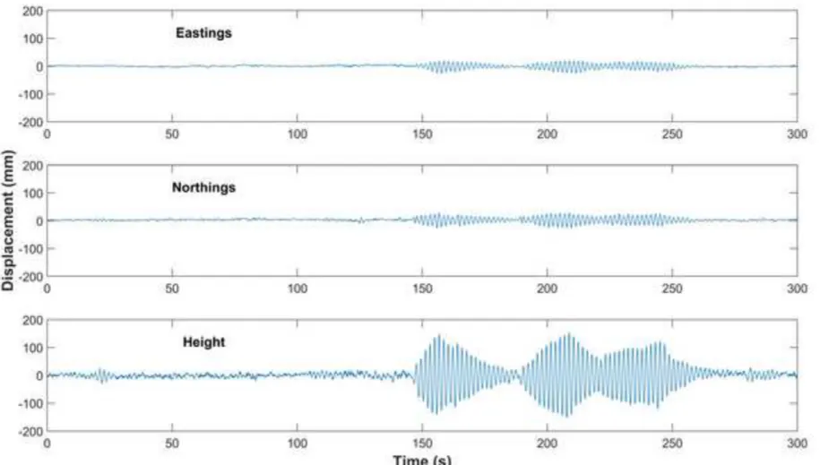
During the experiment, the platform was excited then allowed to move by itself. This meant that the magnitude of the movement decreased over a period of 10s of seconds before re-exciting was required. Figure 5 illustrates the whole of the 8,000 second period of the experiment, illustrating the times that the platform was excited. The period specifically used for analysis in this paper is highlighted in this figure.

Figure 5, The East, North and Height movements of the bungee platform during the whole dataset. The data focussed for illustrative analysis in this paper is within the box.

(9)

1 2 3 4 5 6 7 8 9 10 11 12 13 14 15 16 17 18 19 20 21 22 23 24 25 26 27 28 29 30 31 32 33 34 35 36 37 38 39 40 41 42 43 44 45 46 47 48 49 50 51 52 53 54 55 56 57 58 59 60 61

and Reference 2. Figure 6 (bottom) illustrates the PSD analysis of the same data, again illustrating that there are no relative short term movements between the two pillars. These data can be used as a control for the moving platform, giving an indication of the noise levels expected in the positional solution. There is no movement between these two locations, therefore any apparent movement seen is due to noise, and hence illustrates the noise expected at the Leica bungee solution at the same time. The noise in Figure 6 will consist of the GPS signal and receiver measurement noise, the multipath noise as well as the noise induced into the positional solution due to the geometry of the satellite constellation. The GNSS carrier phase receiver noise has been shown to be at the sub-millimetre level (Roberts et al, 2012). The multipath noise was expected to be reasonably small due to the open environment used at the experiment site, as well as the choke ring antenna used. The RMS values for Figure 6 (top) are 1.34mm, 3.92mm and 3.39mm in the East, North and Height components respectively, for the 300 second dataset. The RMS values for the whole 62,896 epochs are 2.12mm, 2.56mm and 7.36mm for the East, North and Height components respectively. The North component is a little high in the 300 second sample, but in both the North noise is higher than that of the East component. This is an expected phenomenon due to the satellite constellation, and there being gaps in the constellation in the North direction (Roberts et al., 2008).

Figure 6, Results from processing the two Leica GR10 GNSS receivers’ GPS data in an on the fly manner, resulting in 3D coordinates at a rate of 10Hz. The East, North and Height positional results (top) and the PSD analysis for the same data (bottom).

Figure 7 illustrates the Leica based GPS solution (top) and the ComNav GPS based solution (bottom) between the two GNSS receivers attached to the GNSS antenna located at Reference 1, and the two GNSS receivers located to the bungee platform. Figure 8 illustrates the ComNav BDS solution (top) and the ComNav GPS/BDS solution (bottom). It can be seen that they are all very similar in magnitude to each other.

(10)

1 2 3 4 5 6 7 8 9 10 11 12 13 14 15 16 17 18 19 20 21 22 23 24 25 26 27 28 29 30 31 32 33 34 35 36 37 38 39 40 41 42 43 44 45 46 47 48 49 50 51 52 53 54 55 56 57 58 59 60

Figure 7, The Leica GPS solution (top) and the ComNav GPS solution (bottom).

Figure 8, The ComNav BDS solution (top) and the ComNav combined GPS/BDS solution (bottom).

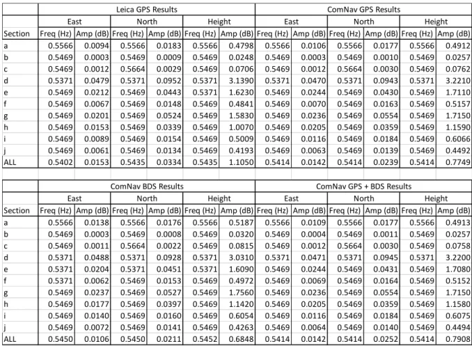
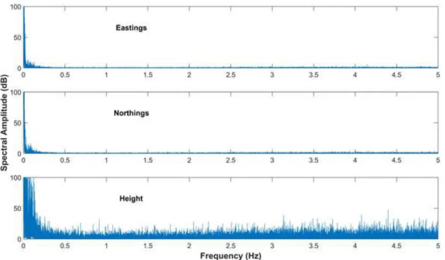
Figure 9, A sample PSD output, illustrating the main natural frequency of the East, North and Height movements of the bungee rig at 0.5469Hz.

Table 2, PSD results for 10 sections of the dataset, where the rig was excited, as well as the PSD for the whole of the dataset.

b. Rotating Arm Results

This section illustrates some of the results obtained from the rotating experiment. The data were processed using RTKLib version 2.4.2 (Takasu and Yasuda, 2009) using a forward solution, with continuous ambiguity resolution. Thus simulating a real time solution where

Section Freq (Hz) Amp (dB) Freq (Hz) Amp (dB) Freq (Hz) Amp (dB) Freq (Hz) Amp (dB) Freq (Hz) Amp (dB) Freq (Hz) Amp (dB)

a 0.5566 0.0094 0.5566 0.0183 0.5566 0.4798 0.5566 0.0106 0.5566 0.0177 0.5566 0.4912

b 0.5469 0.0003 0.5469 0.0009 0.5469 0.0248 0.5469 0.0003 0.5469 0.0010 0.5469 0.0257

c 0.5469 0.0012 0.5664 0.0029 0.5469 0.0706 0.5469 0.0012 0.5664 0.0030 0.5469 0.0762

d 0.5371 0.0479 0.5371 0.0952 0.5371 3.1390 0.5371 0.0470 0.5371 0.0943 0.5371 3.2210

e 0.5469 0.0212 0.5469 0.0443 0.5371 1.6230 0.5469 0.0244 0.5469 0.0430 0.5469 1.7110

f 0.5469 0.0067 0.5469 0.0148 0.5469 0.4841 0.5469 0.0070 0.5469 0.0163 0.5469 0.5157

g 0.5469 0.0201 0.5469 0.0524 0.5469 1.5830 0.5469 0.0236 0.5469 0.0554 0.5469 1.7150

h 0.5469 0.0153 0.5469 0.0339 0.5469 1.0070 0.5469 0.0205 0.5469 0.0359 0.5469 1.1590

i 0.5469 0.0089 0.5469 0.0154 0.5469 0.5009 0.5469 0.0116 0.5469 0.0184 0.5469 0.6066

j 0.5469 0.0061 0.5469 0.0134 0.5469 0.4193 0.5469 0.0063 0.5469 0.0139 0.5469 0.4492

ALL 0.5402 0.0153 0.5435 0.0334 0.5435 1.1050 0.5414 0.0142 0.5414 0.0239 0.5414 0.7749

Section Freq (Hz) Amp (dB) Freq (Hz) Amp (dB) Freq (Hz) Amp (dB) Freq (Hz) Amp (dB) Freq (Hz) Amp (dB) Freq (Hz) Amp (dB)

a 0.5566 0.0138 0.5566 0.0176 0.5566 0.5187 0.5566 0.0109 0.5566 0.0177 0.5566 0.4913

b 0.5469 0.0003 0.5469 0.0008 0.5469 0.0320 0.5469 0.0004 0.5469 0.0011 0.5469 0.0257

c 0.5469 0.0011 0.5664 0.0022 0.5469 0.0815 0.5469 0.0012 0.5664 0.0030 0.5469 0.0758

d 0.5371 0.0488 0.5371 0.0928 0.5371 3.0310 0.5371 0.0471 0.5371 0.0945 0.5371 3.2200

e 0.5371 0.0204 0.5371 0.0451 0.5371 1.6090 0.5469 0.0244 0.5469 0.0431 0.5469 1.7080

f 0.5371 0.0062 0.5469 0.0153 0.5469 0.4972 0.5469 0.0069 0.5469 0.0164 0.5469 0.5152

g 0.5469 0.0237 0.5469 0.0527 0.5469 1.7560 0.5469 0.0236 0.5469 0.0554 0.5469 1.7150

h 0.5469 0.0177 0.5469 0.0397 0.5469 1.1420 0.5469 0.0205 0.5469 0.0359 0.5469 1.1580

i 0.5469 0.0140 0.5469 0.0160 0.5469 0.6054 0.5469 0.0116 0.5469 0.0184 0.5469 0.6075

j 0.5469 0.0072 0.5469 0.0141 0.5469 0.4263 0.5469 0.0064 0.5469 0.0140 0.5469 0.4494

ALL 0.5450 0.0106 0.5450 0.0211 0.5452 0.6848 0.5414 0.0142 0.5414 0.0252 0.5414 0.7908

North Height

East North Height

ComNav GPS + BDS Results

East North Height

Leica GPS Results

East

East North Height

ComNav GPS Results

(11)

1 2 3 4 5 6 7 8 9 10 11 12 13 14 15 16 17 18 19 20 21 22 23 24 25 26 27 28 29 30 31 32 33 34 35 36 37 38 39 40 41 42 43 44 45 46 47 48 49 50 51 52 53 54 55 56 57 58 59 60 61

no backward processing was used. The Javad data is presented in this section. The solutions used here are the GPS only and the combined GPS/BDS solutions.

Figure 10 illustrates the GPS solution over a 600 second time span to show the detail around the time that the rig was initially static, then switched on to start rotating. Figure 11 illustrates the GPS/BDS solutions over the same 600 seconds time span.

Figure 10, the GPS solution over a 600 second time span.

Figure 11, the GPS/BDS solutions over the same 600 seconds time span.

The oscillating nature of the movements in all three components (East, North and Height) are evident in Figures 10 and 11 in particular. These two figures illustrate a section of the positional output in time domain, over a 600 second interval of the whole data. There appears to be a slight line trend on the height component in Figure 10, which doesn’t seem to appear in Figure 11, possibly illustrating an advantage of the combined solution, and improving the geometry of the satellite constellation.

Even though the data presented look similar, there are differences between the two solutions. Figure 12 illustrates the comparison between the two solutions in Figures 10 and 11 for the whole of the 48minute dataset. This includes the rotating arm being stationary up to the 550 second mark, and in a dynamic manner after this time. The RMS values in Figures 12 are 3.16mm, 4.98mm and 11.08mm in the East, North and Height components respectively.

There are anomalies seen (spikes) in Figure 12 at the 933 second, 1678 second and 2817 second marks. These are due to the solution for the GPS only result losing the integer ambiguity value and resorting to a float solution for a few epochs of data. This is not the case for the GPS/BDS solution and illustrates a benefit of the combined solution.

Figure 12, The difference between the GPS and GPS/BDS solutions in the East, North and Height components.

(12)

1 2 3 4 5 6 7 8 9 10 11 12 13 14 15 16 17 18 19 20 21 22 23 24 25 26 27 28 29 30 31 32 33 34 35 36 37 38 39 40 41 42 43 44 45 46 47 48 49 50 51 52 53 54 55 56 57 58 59 60

Figure 13, The PSD analysis results for the GPS solution (top) and the GPS/BDS solution (bottom).

Data Correlation

The rotating rig was set up to rotate at a constant speed. A data correlation function was used in order to determine the nature of the correlation of the oscillating data results. This was carried out by using a section of 500 epochs, of 10Hz data, from the start of the dataset to then correlate with successive sections of 500 epochs, advancing 90 epochs at a time. In all, 190 sections of 500 epochs were used. The total size of the dataset analysed was 33,737 epochs (3,373.7 seconds). The initial 500 epochs of the dataset were used as a reference, and the subsequent 500 epoch sample datasets were correlated against the reference. The algorithm would calculate the lag between the various datasets with the base dataset, correct for this, and directly correlate the datasets with each other. Figure 14 shows an example of the reference and sample data. Here, two of the 500 epoch datasets are illustrated against each other. The offset, lag, is evident in the figure.

Figure 14, Comparison of the reference data (blue) and a sample (red) to be correlated against.

Figure 15 illustrates a correlation example between the reference and one 500 epoch sample. Figure 15 illustrates that the reference correlates with this specific 500 epoch sample at 99.84% value. The two datasets have a 2 second delay. The algorithm is set up to that the sample’s 500 epoch window can move outside of the initial 500 epoch interval chosen, to take into account the lag.

Figure 15, An example of the output for one of the correlation results.

(13)

1 2 3 4 5 6 7 8 9 10 11 12 13 14 15 16 17 18 19 20 21 22 23 24 25 26 27 28 29 30 31 32 33 34 35 36 37 38 39 40 41 42 43 44 45 46 47 48 49 50 51 52 53 54 55 56 57 58 59 60 61

epochs of the data file, but this time during the static period, seen in Figures 10 and 11 from the 400 to 550 second marks. This would result in illustrating the output when the two datasets being compared are not correlated. Therefore, illustrating the difference between correlated and non-correlated data.

Figure 16 illustrates the normalised cross correlation coefficient derived for a number of comparisons throughout the datasets. These are for the GPS only solutions (left) and the GPS/BDS solutions (right). It can be seen that the normalised cross correlation coefficient between the dynamic reference and dynamic dataset varies throughout, but is still at a very high value. Values close to either ±1 are seen as highly correlated, and values close to zero are seen as un-correlated. PSD analysis was carried out on the same 500 epoch samples, and the frequencies in all three of the North, East and Height components were calculated as 0.1172Hz for every single sample. In a perfect scenario, the cyclic nature of the results would be consistent, and the correlation would be equal to 1 throughout. However, this is not the case. There are two main reasons for the discrepancy. The first is that the frequency of the arm’s movement fluctuates. The second is that the 3D coordinates of the position of the GNSS antenna are not precise.

The PSD analysis of all the moving section, consisting of 33,737 epochs of data (51min 13.7s), illustrate that the frequency of the oscillation in the east, north and vertical components are 0.1172Hz. In addition to this, analysis of all the 500 epoch subsets of this dynamic data also conclude that the frequency of the movement is constantly 0.1172Hz. This illustrates the constant and precise nature of the rotating rig, as well as the frequencies derived from the GNSS results.

Figure 16, The normalised cross correlation coefficients for the 190, 500 epoch long samples using the GPS solution (left) and the GPS/BDS solution (right)

Figure 17 illustrates the frequencies calculated using the GPS and BDS data over three sections of data. Test 1 sees the arm rotating at a rate of 0.1172 Hz throughout, already discussed in the paper. Test 2 at a rate of 0.03906 Hz constantly, and test 3 at a rate of 0.07813 Hz constantly are additional pieces of data again showing the consistent nature of the results. These are over periods of 51minutes and 13.7 seconds, 19 minutes and 17 seconds, and 29 minutes and 15 seconds respectively. Between the three tests, the frequency of the movement of the arm was changed, but the results again show that there is consistency in the frequencies derived from the GNSS data for each test.

(14)

1 2 3 4 5 6 7 8 9 10 11 12 13 14 15 16 17 18 19 20 21 22 23 24 25 26 27 28 29 30 31 32 33 34 35 36 37 38 39 40 41 42 43 44 45 46 47 48 49 50 51 52 53 54 55 56 57 58 59 60

5. Discussion and Conclusions

The experiments and analysis illustrate the use of frequency analysis derived from GNSS data and data correlation of displacement in order to measure the movement characteristics of dynamic platforms. The moving platform has a cyclic movement, thus simulating a structure such as a bridge.

The results illustrate that even though the positional solutions may have noise at the millimetre level, frequency analysis and correlation of various pieces of data can be used to determine whether the characteristics of the data are changing. This could be used on a structure in order to analyse changes over time, and hence be used as part of a Structural Health Monitoring system. The results indicate that analysing the displacements derived from GPS or a combined GPS and BDS solution can result in precisions at the millimetre level. The difference between the GPS derived and GPS/BDS derived solutions have RMS values of 3.16mm, 4.98mm and 11.08mm in the Eastings, Northings and vertical components respectively. These relative magnitudes of RMS are as expected, and thought to be due to the geometrical effects of the satellite constellations. This is generally best in the East-West direction and worst in the vertical direction (Meng et al., 2004).

By analysing the trends in the movement data, through using an autocorrelation technique, it can be seen that the correlation of an initial segment of the moving data compares well with subsequent segments of the whole data. The correlation of the results is of the order of 89.2%, 87.9% and 77.5% in Eastings, Northings and Height respectively when using GPS alone. The introduction of BeiDou into the solution has little effect on the plan position, but slightly improves the vertical to 78.9%. Interestingly, the Eastings are the best results, with the height being the worst, again thought to be due to the satellite geometry in particular.

The data correlation could be carried out between different epochs of the same data, or even between different measurement types, using additional sensors. Resulting in the ability to monitor any changes outside of the expected ranges of the movements.

Using a combined GPS and BDS solution introduces some improvement in the positional results, but more so in the height. This is thought to be due to the geometry of the GPS satellites being already good in the horizontal component, and hence little improvement seen here, but due to the different satellite constellation types and inclination angles of the satellite orbits improving the height component slightly more.

The equipment and test rigs have proven useful in order to gather such dynamic and cyclic data, in a controlled environment. The bungee rig, however, could be improved by adding an on-board excitation device, allowing the rig to be automated.

Acknowledgements

‘The work in this paper is supported by the Ningbo Science and Technology Bureau as Part of the Project Structural Health Monitoring of Infrastructure in the Logistics Cycle

(2014A35008)’.

References

(15)

1 2 3 4 5 6 7 8 9 10 11 12 13 14 15 16 17 18 19 20 21 22 23 24 25 26 27 28 29 30 31 32 33 34 35 36 37 38 39 40 41 42 43 44 45 46 47 48 49 50 51 52 53 54 55 56 57 58 59 60 61

Çelebi, M., Prescott, W., Stein, R., Hudnut, K., Behr, J., & Wilson, S. (1999) GPS monitoring of dynamic behavior of long-period structures. Earthquake Spectra, Journal of the Earthquake Engineering Research Institute, 15(1), 55-66.

Chen, J., Zhang, Y., Wang, J., Yang, S., Dong, D., Wang, J., Qu, W. & Wu, B. (2015) A simplified and unified model of multi-GNSS precise point positioning. Advances in Space Research, 55(1), 125-134. DOI 10.1016/j.asr.2014.10.002.

Hofmann-Wellenhof, B., Lichtenegger, H. & Wasle, E. (2008) GNSS Global Navigation Satellite Systems. SpringerWien New York. ISBN 978-3-211-73012-6.

Jin, S. (2013) Recent progresses on Beidou/COMPASS and other global navigation satellite systems (GNSS) – I. Advances in Space Research, 51(6), page 941. DOI

10.1016/j.asr.2012.12.007.

Lovse, J. W., Teskey, W. F., Lachapelle, G., & Cannon, M. E. (1995) Dynamic deformation monitoring of tall buildings using GPS technology. ASCE Journal of Surveying Engineering, 121(1), 35-40.

Meng, X., Roberts, G. W., Dodson, A. H., Cosser, E., Barnes, J. & Rizos, C. (2004) Impact of GPS Satellite and Pseudolite Geometry on Structural Deformation Monitoring: Analytical and Empirical Studies. Journal of Geodesy, 77(12), Publisher: Springer-Verlag Heidelberg, ISSN: 0949-7714 (Paper) 1432-1394, June 2004.

Nadarajah, N. Teunissen, P. J. G. Raziq, N. (2014) Instantaneous BeiDou–GPS attitude determination: A performance analysis. Advances in Space Research, 54(5), 851-862. DOI 10.1016/j.asr.2013.08.030.

Ogundipe, O., Roberts, G. W. & Brown, C. J. (2014) GPS monitoring of a steel box girder viaduct. Structure and Infrastructure Engineering: Maintenance, Management, Life-Cycle Design and Performance, 10(1), 25-40. DOI 10.1080/15732479.2012.692387. ISSN 1573-2479 print/ISSN 1744-8980 online.

Psimoulis, P.A. & Stiros, S.C. (2008) Experimental assessment of the accuracy of GPS and RTS for the determination of the parameters of oscillation of major structures. Computer-Aided Civil and Infrastructure Engineering, 23(5), 389-403. DOI 10.1111/j.1467-8667.2008.00547.x.

Psimoulis, P., Pytharouli, S., Karambalis, D, & Stiros, S. (2008) Potential of global positioning system (GPS) to measure frequencies of oscillations of engineering structures. Journal of Sound and Vibration, 318(3), 606-623. DOI 10.1016/j.jsv.2008.04.036.

Rizos, C., van Cranenbroeck, J. & Lui, V. (2010) Advances in GNSS-RTK for Structural Deformation Monitoring in Regions of High Ionospheric Activity. In Proc.: FIG Congress “Facing the Challenges – Building the Capacity”, Sydney, Australia.

(16)

1 2 3 4 5 6 7 8 9 10 11 12 13 14 15 16 17 18 19 20 21 22 23 24 25 26 27 28 29 30 31 32 33 34 35 36 37 38 39 40 41 42 43 44 45 46 47 48 49 50 51 52 53 54 55 56 57 58 59 60

Roberts, G.W. Meng, X. Dodson, A.H. (2004) Integrating a Global Positioning System and Accelerometers to Monitor the Deflection of Bridges. Journal of Surveying Engineering, American Society of Civil Engineers, 65-72, May 2004,Vol 130, No 2, ISSN 0733-9453.

Roberts, G.W. Meng, X. Brown, C.J. Dallard, P. (2008). GPS measurements on the London Millennium Bridge. Proceedings of the Institution of Civil Engineers, Civil Engineering Innovation, ISSN 1755-0890, 2(1), 15-28.

Roberts, G. W.; Brown, C. J.; Meng, X.; Ogundipe, O.; Atkins, C.; and Colford, B.; (2012). Deflection and frequency monitoring of the Forth Road Bridge, Scotland, by GPS. Proceedings Institution of Civil Engineers; Bridge Engineering, 165(2), 105-123. DOI 10.1680/bren.9.00022. ISSN: 1478-4637, E-ISSN: 1751-7664.

Roberts, G. W.; Brown, C. J.; Tang, X.; Meng, X.; Ogundipe, O.; (2014) A Tale of Five Bridges; the use of GNSS for Monitoring the Deflections of Bridges. The Journal of Applied Geodesy. 8(4), 241-264. DOI 10.1515/jag-2014-0013. ISSN 1862-9024.

Takasu, T. & Yasuda, A. (2009) Development of the low-cost RTK-GPS receiver with an open source program package RTKLIB. International Symposium on GPS/GNSS, International Convention Center Jeju, Korea, November 4-6, 2009. CD-ROM.

Teague, E. H., How, J. P., Lawson, L. G., & Parkinson, B. W. (1995) GPS as a structural deformation sensor. In Proc: The AIAA Guidance, Navigation and Control Conference, Baltimore, MD; UNITED STATES; 7-10 Aug. 1995. ISSN 0146-3705, pp 787-795.

Tu, R., Wang, R., Ge, M., Walter, T. R., Ramatschi, M., Milkereit, C., Dahm, T. (2013). Cost-effective monitoring of ground motion related to earthquakes, landslides, or volcanic activity by joint use of a single-frequency GPS and a MEMS accelerometer. Geophysical Research Letters, 40(15), 3825-3829. DOI http://dx.doi.org/10.1002/grl.50653.

Tu, R., Ge, M., Wang, R., & Walter, T. R. (2014). A new algorithm for tight integration of real-time GPS and strong-motion records, demonstrated on simulated, experimental, and real seismic data. Journal of Seismology, 18(1), 151-161. DOI http://dx.doi.org/10.1007/s10950-013-9408-x.

Vaclavovic, P. & Dousa, J. (2015) Backward smoothing for precise GNSS applications. Advances in Space Research, 56(8), 1627-1634. DOI 10.1016/j.asr.2015.07.020.

Verhagen, S. & Teunissen, P. J. G. (2014) Ambiguity resolution performance with GPS and BeiDou for LEO formation flying. Advances in Space Research, 54(5), 830-839. DOI 10.1016/j.asr.2013.03.007.

Xiao, W., Liu, W., & Sun, G. (2016) Modernization milestone: BeiDou M2-S initial signal analysis. GPS Solutions, 20(1), 125-133. DOI 10.1007/s10291-015-0496-7.

(17)

1 2 3 4 5 6 7 8 9 10 11 12 13 14 15 16 17 18 19 20 21 22 23 24 25 26 27 28 29 30 31 32 33 34 35 36 37 38 39 40 41 42 43 44 45 46 47 48 49 50 51 52 53 54 55 56 57 58 59 60 61