Computation of the Multivariate Normal Integral over a Complex Subspace

Computation of the Multivariate Normal Integral over a

Complex Subspace

Kartlos Joseph Kachiashvili1,2_{, Muntazim Abbas Hashmi}3

1_{Abdul Salam School of Mathematical Sciences, GC University, Lahore, Pakistan} 2_{Vekua Institute of Applied Mathematics, Tbilisi State University, Tbilisi, Georgia}

3_{Air University Multan Campus, Multan, Pakistan} Email: [email protected], [email protected]

Received January 25,2012; revised March 30, 2012; accepted April 6, 2012

ABSTRACT

The computation of the multivariate normal integral over a Complex Subspaceis a challenge, especially when the

inte-gration region is of a complex nature. Such integrals are met with, for example, in the generalized Neyman-Pearson criterion, conditional Bayesian problems of testing many hypotheses and so on. The Monte-Carlo methods could be used for their computation, but at increasing dimensionality of the integral the computation time increases unjustifiedly. Therefore a method of computation of such integrals by series after reduction of dimensionality to one without informa-tion loss is offered below. The calculainforma-tion results are given.

Keywords: Multivariate Normal Integral; Random Variable; Probability; Moments; Series

1. Introduction

At testing many hypotheses with reference to the pa- rameters of multivariate normal distribution, the problem of computation of multivariate normal integrals over a

Complex Subspaceof the following form arises [1]





d , , 1, , , ,

j

ij i

p p H i j S i





_

x x    j

,

(1)

where is the number of tested hypotheses

i supposing that sample

S

i θ

:

H θ xT 



x₁, , x_n



was

brought about by distribution

  

, 1, , ; , ,1







, 1,

i i i

n m i

p xθ  p x  x    p xH i ,S



where



1, ,

T

m

  

θ 

 is the vector of distribution pa-

rameters and i is the acceptance region of hypothesis

i

H from sample space , which has the fol-

lowing form

n

R



xRn













: 1,

1, ,

S

j j

j k pj Hj jk p H

j S

 

  





x x    x 





,

(2)

where 0_kj  , .

 1, , S

Such regions of hypotheses acceptance arise, for ex- ample, in the generalized Neyman-Pearson criterion, and also in conditional Bayesian problems of testing many hypotheses [2,3]. The dimensionality of these integrals often reaches several tens when practical problems are solved. For example, in ecological problems the number of controlled parameters, according to which the decision

is made, is quite often equal to several tens [4]; in the air defence problems, in particular, in the problems of tracking of flying objects using radar measurement in- formation, the dimensionality of the problem is equal to the multiplication of the number of flying objects by the number of surveys made by the radar set [5] and so on. On the other hand, the time for solution of these prob- lems is often limited and at times it plays a decisive role especially at solving the defence problems.

It is known that the complexity of realization and the obtained accuracy of numerical methods of computation of multidimensional integrals depend heavily on the di- mensionality of these integrals and the complexity of the integration region configuration. In the considered case the integration regions are nonconvex and quite complex. Therefore it is difficult to realize the numerical methods and to provide the desired accuracy of calculation even when the dimensionality of integral is greater than or equal to three [6]. The methods of computation of the multivariate normal integral on the hyperrectangle of- fered in [7-12] are unsuitable for this case because of the complexity of the integration region.

The aim of the present paper is the development of the method of computation of probability integral (1) with the desired accuracy in a minimum of time.

2. Problem Statement

Let us consider the case when the probability distribution

density of the vector x looks like





 

_2π /2 1/2_exp 1





1





_,

2 1, , ,

i

T

n i i

i i

p H

W

i S



  

 _ 

 

x

x a W x a





 _



   

0

(3)

where





2

1 12 1

2

21 2 2

1

2

1 2

, , ,

i i i

n

i i i

iT i i n

n i

i i i

n n n

a a

  

  

  

  

 _{ }

 

 

 

a W

  

   



.

For probability distribution density (3), let us rewrite decision-making region (2) as







: 1 exp



S j

j C y

  x



     , (4)

where

 

 

1 2 /2

1 2 /2

2π , ,

2π ,

n j j

n

j j

j j j

C k j

C k

 

 

 

 

W W

   





1





1 _{, , 1, ,}

2

T

y_ x a  W_ x a   j  S S

. (5)

Random variables , are squared forms

of the normally distributed random vector, and, if hypothesis

, 1, ,

y_  

i

H is true, their mathematical expectations

are equal to

















1

1

1 2 1

trace , , 1, , .

2

T

i i

i

i

E y H

i S





  

 

a a W a a

W W

 

 

  

(6)

Therefore, if hypothesis H_i is true, the random

variable y_ has noncentral distribution 2 with the

degree of freedom and with the parameter of non-

centrality equal to (6) [2,17,18]. n

It is obvious that, at i and hypothesis H_i is true,

the random variable y_i has the central 2 distribution

with the degree of freedom n.

Let us write down (1) as follows





d



1 exp







j

S j

ij i i

p p H P _C y H





_

x x



_{ }  _ 0

 

(7)

The task consists in the computation of probability (7). The method of its analytical computation is not known so far. For its computation it is possible, for example, to use

a modified Monte-Carlo method (with the purpose of

reducing the computation time) [3]. Though, at large ,

it still takes a good deal of time. The method of com- putation of probability (7) if hypotheses are formulated with reference only to the mathematical expectation of normally distributed random vector is offered in [3]. This method is unsuitable here, as the random variable

S





1 exp ,

S j

j C y

 



_  (8)

which formulates integration region (4), in [3] is the weighted sum of log-normally distributed random quan-

tities; j

C_ and are determined by formulae (5). In

our case,

y_

j

 is the weighted sum of the exponents of

negative quadratic forms of the normally distributed random vector with correlated components.

Let us consider the case . In this case, regions (2)

take the form

2

S 













1 :p H2 k p1 H ,

  x x  x 1













2 :p H1 k p2 H .

  x x  x 2

With taking into account probability densities (3), for these regions we derive



1 1



2 1 1 1





1 : 1 2 2 2 1

T T T T

W ₁₂ ,

   

  x x W x x x a W a W x



1 1



1 1 2 1





2 : 2 1 2 1 2 21 ,

T T T T

W 

   

  x x W x x x a W a W x where





1 2

1 2 1 2 1 1 1

12 1 1 2 1

2 2

2 ln T T ,

k 



 



 

 

 _{ } 

 

 

W

a W a a W a W





1 2

2 1 1 1 2 1 2

21 2 1 1 2

2 1

2 ln T T

k 



 



 

 

 _{ } 

 

 

W

a W a a W a W

.

Let us designate





1 1 2 1 1

12 1 2 2 2 1

T T T T 1

x  _{x W x x W x} _  _{ a W} _{a W} _,





1 1 1 1 2

21 2 1 2 1 2

T T T T

 _{x W x x W x} _  _{ a W} _{a W}1 _x.

Then, finally, for the required regions, we shall obtain





1 :12 1 ,

  x  2





2 :21 21

  x  .

Each of random variables 12 and 21 is the sum of

three random variables one of which is distributed by the

normal law, and the two others are distributed by the _2

law. Therefore, the probability distribution laws of ran-

dom variables ₁₂ and ₂₁ have not closed forms.

Thus, at S2, i.e. at testing two hypotheses with

bution (in contradistinction to the case when hypotheses are formulated with respect to only the vector of mathe- matical expectation [3]), the principal complexity of the considered problem does not decrease.

3. Computation of Probability Integral (7)

by Series

Let us use the expanded form of representation of the quadratic form in (8) [18,19]. Then

1 1 2 2

1 2

1 2 1 2

,

1 1 1

1 exp

2

S n n

t t t t

j

j t t

t t t t

x a x a

C

 

 

  

     

 

  _ _ 

   

 





  

  



 

 (9)

where t t_{1 2},

 _{are the coefficients determined unambi-}

guously by the elements of matrix W_ (see formula (3)).

Let pj



z|Hi



be the conditional density of pro-

bability distribution of the random variable j. Then,

for (7), we obtain





0

| d

ij j i

p 



_p z H z. (10)

Here the infinite interval



 ,



is taken as the

domain of definition of random variable j because of

the signs of coefficients j

C_ from (5).

As was mentioned above, the probability distribution

law of the random variable j has not a closed form.

Let us consider the opportunity of approximating this density by series. For this reason we need the moments

of the random variable j [19-21]. Let us consider the

problem of obtaining of these moments.

With this purpose let us calculate the initial moment of

the rth order of random variable _j provided that

hypothesis Hi is true

 













1 1

1

,

1

1 1

exp

exp ... ,

1, 2,

r r

r S

r

j i j

r j i

S S

j j

i

E H E C y H

C C E y y H

r

 



 

_{ } 

  _

 _{ } _  _

  _  _



 _  





 

 



   

 

 



r

i





 _ (11)

Expression ₁

r

y_   y_ is the sum of correlated

Quadratic Forms distributed by noncentral _2 _pro-

bability distribution laws. Because of correlation, the

property of reproducibility of the _2 _{distribution does}

not take place [2,18], and, consequently the mathematical expectation in (12) has not a closed form.

Let us use power series expansion of the exponent









 



 



 

1 1 2

1 2

1

0

0 ,. , ; 1, ,

1

exp 1

! 1

1 .

!

r r

i r

p p p

p i

y y y y y

y y y_

 





 

 



 

  

       

  







    

   

 



(12)

Let us use the expanded representation of quadratic

form (9) and be satisfied with the first M terms of ex-

pansion (12). Then expression for calculation of mo- ments (11) can be represented as follows

1 1

1 1 2

1 1 2

1 2

,

1 1 1

, { , , }; 1, , 1 1

, 1

1 1

2

1 !

,

r r

i r

S S M

j i j j

r

n n p t t

p i t t

m p p

t t p i

C C

x a

E H

  









 

 _



 





  

   







      _ _

 

 

 

   _{  } 

 

 _{ }  _

  _ _  _



  _

 









   

   

 





(13)

where  



1, , 2 , 



m_



0,1, , 2 



and

1m 2

 



 



.

Expression (13) contains product moments [17,19,20]

of the 2 ( 1, , M) orders of normalized compo-

nents of the correlated normally distributed random ob- servation vector. Therefore, they are not equal to zero [18]. A lot of works are dedicated to the problem of com- putation of product moments [see, for example, 22-28].

In [22] the following problem was solved. Let

1, , ,2 n

x x  x

tions, and let

be random variables with mutually indepen- dent distribu

1

n i i

X x







. There is found the

probability that X lies between A and B , i.e.





P AX B , by sing the central limit theo in

h which the random variable

ln n ln i

u rem

accordance wit

1

i

X 



x is approximately distributed



by the nor-

mal law. The better is this approximation the bigger is

he variance of the product of two random variables w

n.

T

as studied by Barnett (1955) and Goodman (1960), in the case when they do not need to be independent. Shel- lard (1952) studied the case when the distribution of

k

1 i

i

x





was (approximately) logarithmic-normal. The au-

1, , ,2 n

x x  x

ndent distri

thor considered the case when are random

variables with mutually indepe butions. For

finding the probability that n

1 i

i

X x







lies between A

and B, i.e. P A



X B



ach the probab

, the central limit theorem is

used appro ility distribution of the ran-

dom variable ln

to

X by normal distribution and this ap-

proach is better at increasing n. In work [25] no assump-

tion is made about the distribut k

1

i i

x





. There is dis-

ion of

K random variables,

1, , ,2 k

x x  x ,



K2



are mutu y independent, and

en not have to be independent, and

there are obtained their variance formulae. These results are generalizations of the results presented in [24].

In [26] are given exact formulae for the mathem all

atical the case wh

ex

they do

pectation of



xiXi





xjXj





xkXk



and



xiXi





xjXj





xkXk



xhXh



,



i  j k h



, where x_i is the sample mean of the

p

ith “character

pu

” in a sam le of n elements from a po-

lation of N elements and X_i is the corresponding

population m n. Formulae for estimating these product moments from the sample were also given. These estima- tions are slightly biased. In [27] the unbiased estimate of the 4-variate product moment was obtained. Asymptotic results for the 3-variate and 4-variate product moments and their estimates were also obtained.

In [28] is derived a formula for the ea product moment 1 1 p m m p EX vival functio X

 , m11, , mp1 in terms of the joint sur-

n when



X₁, ,Xp



is a non-negative

random vector. From the given re



view (of course incomplete, because th

t of the

is is not the aim of this paper) of the works dedicated to the study of product moments, it is seen that the problem considered here differs from them.

Theorem 3.1.The initial momen

r

th order of random variable j determined by (9), provided that

hypothesis Hi is t e, can be calculated with any speci-

fied accuracy y the formula ru b    

 

1 1 1 1 2

1 1 2

1 2 1

,

1 1 1

, , , ; 1, , 1 1

, ,

, , ,

0,1,2, ,2 ; 1, ,

1 1 0 1 1 1 1 2 !

, 1, 2,3,

r r

i r

i

S S M

j i j j

r

n n p t t

p i t t

p i i

t t i j j C C J d r j                                             _ _          _          _

 













               (14)

where Ji, modKi,

 

βi, 1 ; βi,2 and Ki,2 are rices of eigenvectors an

the mat d values of the in- verse covariance matrix of normalized random variables

eigen

, 1, ,

p

x a _{   ;} i,

d

p_ 

 1, ,

 _,



_{0,1, 2, , 2 ,}



 i  

1, ,

i  ,

of matrice

are the coefficients determined by the terms s βi,2 and Ki,2 and vector _bi,2 _;

1 

and _j are th initia central mome f t

first _ j

e l and nts o he

and   orders, respectively, defined by for- mulae (22), nd (24).

Proof. If hypothesis

(23) a

is true, the values ,

p p

x a 

 



 

1, 2, , ,

i

H

    are correlated normally distribut

m variables with the p ameters

ed

ran-do ar

 

 

, _,

p i p

i p i

p p

a a

E H b

              _         2 ,

2 , 1, ,

i p i p i p p x a x a

V H v

   _       _    _  _  _             ； 1 2

1 1 2 2 1 2

1 2 1

1 2 1

1 2

1 2

,

, ,

, 1 2

cov ,

, , 1, , .

p p i

i

p p p

i p p

x a x a

H v                         _{     }           _{   }  _       2 2 p 

 (15)

Thus, for calculation of moments (13), it is required to

calculate the product moments of -dimensional







1, , 2 ,   1, , M



normally distributed ran-

dom vectors for which the components of the vectors of mathe atical expectations and the covariance matrices are calculated by formulae (15).

Let us designate

  

m







₁

 _,

1

, ,

,

1 , ,

T i p i p i

b b

_

b 

1 1 1 2 1

2 1 2 2 2

1 2

, , , , , ,

1,1 1,2 1,

, , , , , ,

2,1 2,2 2,

,

, , , , , ,

,1T ,2T ,

i p p i p p i p p i p p i p p i p p i

i p p i p p i p p

v v v

v v v

v v v

           _                V       

, (16)

and the corresponding random vector—by

i.e.



1, ,



T

y y_



y  ,

1 2

1 1 2 2

1 2

1 2

1 2

p p

x a x a p

p p p

x a

y y y

              ， ，  .

For calculation of conditional product moments o e

，

f th

2-order, we have



1 2



1 2

1 2 1 2

m m m m m m

i

E y y y  H y y y 

 

 

 

_{ }

 



1, , ,2 i



d d1 2 d ,

f y y y H y y y

 

 

  

(17)

where f y y



1, , ,2  y



ability distribution

is the -dimensional

prob density vector of math-

expectations and  with the

normal

ematical the covariance matrix cal-

culated by formulae (16).

It is known that the value of integral (17) is invariant

to linear transformation of the components of vector x

[18] with the accuracy of Jacobian of Transformation. Let us designate the matrixes of eigenvectors and eigen-

values of matrix

 

_Vi, 1 _by i, i

j







 _

β and

, i i j k    , i 

K , respectively. It should be pointed out that



dimensional random vector

  

1



, , , ,

i _ i i  _ i

Z β K y b , ( )

will be uncorrelated and wi

18

ll have standard normal dis- tribution of probabilities [3,20].

From (18), we write

 

1

, , , ,

i i  i i

 

y K β Z b .

Let us introduce the following designation

 

1

.

, , , ,

i i i i

j



 _  _  

γ  K β

the following expression

n (19), for mathematical expecta- tion (17), we obtain



Then, for the elements of the vector y, we obtain

, , , ,

1 , 1 ,

i i i

t t t

y  z b 

   







  . (19)

Using transformatio

,









1 2 ,

1 2

m m m i

i

E y y y  H 

     J , , , , 1 1 , m

i i i

t t i

t

E _ __z  b_  H 

 _  _









(20)

where _Ji, _modKi,

 

_βi, 1 _{is the Jacobian}

Transformation (18).

s raise to the powers the l

n (20) and group the identical of

Let u inear forms in the right-

hand side of expressio

items. Then (20) can be written as





 

 

1 2

1m 2m m i

E y y y  H

     1 , , ,

, , 1 0,1,2, ,2 ; 1, ,

,

i

i i i

i i

d   E z  H

               





J    (21)

where, the coefficients of the identical items in (20) designated by are 1 , , , i

d__ , i



0,1, 2, , 2 ; 



i1, ,

,

i

 ;

the items of the vector Z  are determined as





,

1, , . i

z 

       _{ }  







,



, ,

1 1 ,

i p i i K y     

_

    

 b

It is known that [21,29]

 

 

, 1 0 , i i j j j

E z H

j                   _{ }          



(22)

where _ and j are the initial an

ment

d central mo-

s of  and   j

, orders, respectively, of ran-

dom variable i

z. Af se

ter simple routine transformations, for the considered ca we obtain

 

 

, ,

0, if jis odd.    (23) Here 2 !

,if is even, 2 ! 2 j i z j j j j j       

















2 1

1 2 1 2 1

1 2 , , , , , , , , 1 1 2 , , , , 1 ,

, 1 , ,

, , , , 1 , , . i i i z

i p i p i p

i i

i p i p i

i i i

i p i i i p

V z H

C D b b

C b D

C K

D K b

                                       

 







                      2 2 ,   (24)

Taking advantage of ratios (21), (22), for computation of the moments (13), we obtain expression (14).

Probability integral (10) can be computed with the help of Edgewort’s series [19-21] using formula (14) for computation of the initial moments of random variable (9). In particular, in the considered case, using well- known techniques of obtaining Edgewort’s series [30], we have









 

 

 





 

 





0 *

1 d πˆ 0 1

1

j i j i

i i

p z H z H z

     

 

 





 

 





   

 

3 _{*3 *} 4 _{*4 *2}

1 1 1 1

3/2 2

, ,

2 2

2

3 _{*6 *4 *2}

1 1 1

3 2 , 2

5 _{*5 *3 *} 3 4

1 1 1

5 2 7 2

, ,

2 2

*7 *5

1 1

1

3 6 3

3! 4!

10 _{15 45 15}

6!

1 _{10 15} 35

5! 7!

21 1

j j

j i j i

i j j i

i i i

j

j j

j i j i

z z z z

z z z

z z z

z z                        _{ }                   







 

 





 

 





 

 





 

 

3 3 *3 *

1 1 _, 3 2

2

*9 *7 *5 *3 *

1 1 1 1 1

2

6 *6 *4 *2 4

1 1 1

3 2

, ,

2 2

*8 *6 *4 *2

1 1 1 1

2 3 4 , 2 280 05 105 9!

36 378 1260 945

1 35

15 45 15

6! 8!

28 210 420 105

2100 10! i j j i i i j j

j i j i

i i j j j i

z z

z z z z z

z z z

z z z z

               _{ }                   _{ }                  





 

 







 

*10 *8 *6

1 1 1

5

4 3

*4 *2

1 1 _, 3 2

2

*12 *10 *8 *6

1 1 1 1

*4 *2 *

1 1 1

45 630

23100

3150 4725 945

12!

66 1485 13860

51975 62370 10395 ,

i j j i

z z z

z z

z z z z

z z z





* , ,

where 1 1 2

j i j

z    i ;

 

_k i

j

 , is the

th semi-invariant of the ra





1, 2,

k 

ariable

k ndom v _j provided

ypothesis

h Hi

difficu

is true (the c -invar-

ts is not lt knowing nclude-

omput all in

ation of semi itial moments i ian

ing j i,

k

 (see, for example, [21])); ,

2

j i

 is the second

o

central m ment; 

 

x is standard normal density, i.e.

 



2



x exp x 2 2π.

Satisfying the first seven terms in expansion (25), the absolute value of calculation error of the probability in- tegral is calculated by the formula



 

 





 

 





 

 





 

 

6 _{*6 *4 *2}

1 1 1

3 , 2

2

4 _{*8 *6 *4 *2}

1 1 1 1

2 , 2

2

3 4 _{*10 *8 *6 *4}

1 1 1 1

5 , 2

3 *2

1 _, 3/2

2

1

15 45 15

6!

35

28 210 420 105

8!

2100

45 630 3150

10! 23100 4725 945 12! i j j i j i i j j i i i j j j i i j j i

z z z

z z z z

z z z z

z                        _{ }                           







 

 4

*12 *10 *8 *6 *4

1 1 1 1 1

*2 *

1 1

66 1485 13860 51975

62370 10395 .

z z z z z

z  z

  

   

 

The variable is continuous

and unambiguousl 1





e of

exp

S j

j C y

 



_{ }  _

y defined for every valu x. There-

fore, the random variable j is continuous

of the random variable

. T harac-

teristic function

he c

j

 an its deri-

f any or

tio o di e d any o

vatives o s t m rder of

this random variable exist. At the same time, the chara- cteristic func n is uniformly continuous. Consequently, the distribution function of this random variable exists and is c ntinuous [21].

Theorem 3.2.The stribution function of random va- riabl

der exist, a he mo ents of

j

 exists and is u uely determined by moments

(14).

niq

Proof. For proving this theorem, it is necessary to

show that all moments j i,_{, 1, 2,}

r r

   exist and the fol-

lowing condition takes place [19,21]

 

_, 1 2

2 lim sup 2 r j i r r _r    .

The fact that all moments exist is obvious from for- mula (14) as by using it, it is possible to calculate the moments of any order with any specified accuracy. The values of these moments exist and are finite.

When solving the practical problems coefficients

take on the values bounded above; correlation matrices are positively determined matrices the determinants hich differ from zero. Therefore, coefficients

k

k_

W_

of w j

C_

are bounded-above quantities. There takes place









 





1 1 exp

, d ,

r r y y i i i

E y y H e

N        _{   } _     

 

x a W x

 

  

where ₁

r y_  y_

lly distributed

is the sum of quadratic forms of

ma -dimensional vector

nor n x at dif-

nt t atical expectations and covar-

, at changing compon ts of the or

fere iance m vect

vectors of ma atrices. Ther

hem

efore en

x from 

r

up to , the quadratic form

1

y_   y_ takes the valu om 0 to , and the

e of function

es fr 

valu



y1 yr



e   varies from 1 to 0, res-

pectively. Therefore [18]











,



d 1

i i i N     1 exp _r

E_  y  y H _



_{ }

 x a W x

Thus, taking into account (5) and (11) we can write down   

 

 

1 1 , 1 1 , r r S S

j i j j

r C C



 

1

1 2

1 1 1

2π r r S S nr r

A p H_{ }



 

  



  

 W

   where 

 

_{ }    

A is the maximum by absolute value among

coefficients j

k_ .

Assume r1, then we have

 

 

1

, ₂

1

1

2π n S

j i

A p H

  







 W



.

us designate

Let min _{{ }} 

 

min



W W . Then

 

 

1 1

, _{2 2}

1 min min

1

2π n S 2π n

j i

A p H A

    



 W



  W



.

If

 

2

min

2π n

A W , then ₁j i, 1 and it is not diffi-

to be convinced that j i, ₀

r

  at r .

Let

 

cult

2 _min

2π n

AC W , where C1. Hence

,

j i r

_r C Sr and

 





 

 

 

1 2 1 2

, 2 1/2 1 2

2

1 2 2 1

1 2 ₂

2 1

2 2

2 2 2

2 0

r r

j i r r r

r r r r r r

C S r CS r

r r r

CS C CS r           2 2

at r , which prov s the theorem.

4. Computation Results

The acc acy of this algorithm depends heavily on e

ur M -

of used items in expansion (12 n order to

the number ). I

cy of appr

increase the accura oximation of the exponent

for given M and, in general, the reliability of

putation in the tasks of hypotheses testing, it is expedient to perform first the normalization of initial data by formulae:

com-

 











,

, , 1, ,

ij ij di ci dj cj i j n

  _    _   where

i i i i

x  x c d c

are the minimum and maxi-

mum v parameter for the given set of the

considered hypotheses, i.e.

, i i

c d ,

alues o

1, ,

i  n,

f the ith

 

{ }

min j

i i

j

c  a ,

 

}

max

{

j i

j

d  ai , [3]. In this case, the values of

m and seven items

ansio

am his fact was estab-

lis odel ation vector with non-

correlated components. Unfortunately, by now the con- sidered algorithm has been realized only for such a case [31].

ulation showed that the time of exe- cution of the task (decision-making and computation of the suitable value of the risk function) by using e

Monte-Carlo method made up sec, se

and sec for the numbe ypoth

1, ,

i  n,

the parame

1, ,

j  S

ters of the algorith M 15

in exp n (25) provided the absolute error of com-

putation of integral (1) that does not exceed 0.005 for

computed ex ples (see below). T

hed by m ing for the observ

The results of sim

th c, 1.2

 r of h

4.5 

eses S

13

 3,

re ely

g equal

d co x

n table ,

respectively. Figures are pres

o ses test of the statistical software in

e a propriate method , there are ch

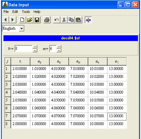
[image:7.595.308.538.86.313.2]

of the tables of these Figures. In the first colum of the

table of Figure 1 is given the vector of measurements

and in the other columns are given hypothetical values of mathematical expectation of this vector.

eanw offered here, the

and the re- noticeably less than 1 sec.

rac 4

 spectiv dimensionality of

S

S

of the whic othe

and

are

task h th r valu

5

S ,

given i

p

es of S

, the

rrelation m

s are reali osen th

the observed vector bein to n

The tested hypotheses an

8  atri

ented as the suitable form in all cases. for th

ur

zed

e suitable sub-sets e case

e 2

s

[31]. For 5

 s of Figure 1 and Fig

f hypothe

n

M hile, when using the method

computation time did not practically change sults were obtained for the time

In both cases probability integrals (7) were computed

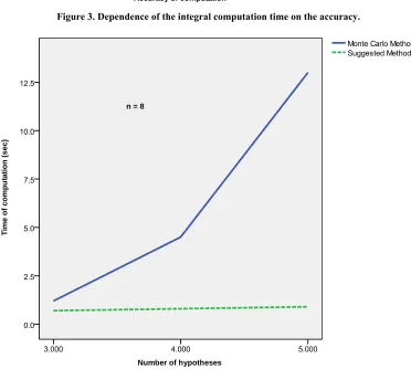
with the accuracy of 0.005. In Figures 3 and 4 are

given the dependences of the integral computation time

on the accu y and number of tested hypotheses respect-

tively.

At solving many practical problems, especially mili- tary problems [5,32], the dimensionality of the integrals

Figure 1. The form of entering the tested hypotheses and a measurement vector.

Figure 2. The form of entering the covariance matrix.

like (1) often is equal to several tens and difference bet- ween the computation time necessary for the considered methods is significantly longer than in the above men- tioned case [14], whereas the computation time for solv- ing the defence problems are of great importance.

The theoretical investigation of the dependence of the

accuracy of computation of integral (1) on M-the num-

ber of items in expansion (13) is a challenging task. There- fore, at program realization of the offered algorithm and,

[image:7.595.309.538.352.588.2]

Accuracy of computatio

n = 8, S = 5

T

ime o

f co

mp

u

tat

io

n

(s

ec

)

[image:8.595.109.483.95.514.2]

n 0.005 0.010

Figure 3. Dependence of the integral c

0.050

omputation time on the accuracy.

Number of hypotheses

T

ime o

f

compu

ta

tion

(s

ec)

n = 8

[image:8.595.109.481.385.719.2]

make parameter M and the number of items in expan-

sion (25) external parameters of the program. This allows establishing their optimal values for each concrete case by experimentation depending on the desired accuracy of computation.

5. Conclusion

The method of computation of the probability integral from the multivariate normal density over the Complex Subspace by using series and the reduction of dimen- sionality of the multidimensional integral to one without losing the information was developed. The formulae for computation of product moments of normalized normally distributed random variables were also derived. The ex- istence of the probability distribution law of the weighted sum of exponents of negative quadratic forms of the nor- mally distributed random vector was justified. The op- portunity of its unambiguous determination by the com- puted moments was proved.

REFERENCES

[1] S. Thompson, “On the Distribution of Type II Errors in Hypothesis Testing,” Applied Mathematics, Vol. 2, No. 2,

2011, pp. 189-195. doi:10.4236/am.2011.22021

[2] C. R. Rao, “Linear Statistical Inference and Its Applica-tion,” 2nd Edition, John Wiley & Sons Ltd, New York, 2006.

] K. J. Kachiashvili, “Generalization of Bayesian Rule of Many Simple Hypotheses Testing,” International Journal of Information Technology & Decision Making, Vol. 2,

No. 1, 2003, pp. 41-70. doi:10.1142/S0219622003000525 [3

[4] A. V. Primak, V. V. Kafarov and K. J. Kachiashvili, “System Analysis of Air and Water Quality Control,” Naukova Dumka, Kiev, 1991.

[5] A. I. Potapov, A. G. Vinogradov, I. A. Goritskyi and E. E. Pertsov, “About Decision-Making of Presence of Objects at Group Measurements,” Questions of Radio-Electronics,

Vol. 6, 1975, pp. 69-76.

[6] P. J. David and P. Rabinovitz, “Methods of Numerical Integration. Computer Science and Applied Mathemat-ics,” 2nd Edition, Academic Press Inc., Orlando, 1984. [7] A. Genz, “Numerical Computation of Multivariate Normal

Probabilities,” Journal of Computational and Graphical Statistics, Vol. 1, 1992, pp. 141-149.

[8] A. Genz, “Comparison of Methods for the Computation of Multivariate Normal Probabilities,” Computing Science and Statistics, Vol. 25, 1993, pp. 400-405.

[9] A. Genz and F. Bretz, “Numerical Computation of Mul-tivariate t-Probabilities with Application to Power Calcu-lation of Multiple Contrasts,” Journal of Statistical Com-putation and Simulation, Vol. 63, No. 4, 1999, pp. 361-

378. doi:10.1080/00949659908811962

[10] S. Joe, “Approximations to Multivariate Normal Rectan-gle Probabilities Based on Conditional Expectations,”

Journal of the American Statistical Association, Vol. 90,

1995, pp. 957-964.

[11] I. H. Sloan and S. Joe, “Lattice Methods for Multiple Integration,” Clarendon Press, Oxford, 1994.

[12] V. Hajivassiliou, D. McFadden and P. Ruud, “Simulation of Multivariate Normal Rectangle Probabilities and Their Derivatives: Theoretical and Computational Results,”

Journal of Econometrics, Vol. 72, No. 1-2, 1996, pp. 85-

134. doi:10.1016/0304-4076(94)01716-6

[13] J. O. Berger, “Statistical Decision Theory and Bayesian Analysis,” Springer, New York, 1985.

[14] K. J. Kachiashvili, “Bayesian Algorithms of Many Hy-pothesis Testing,” Ganatleba, Tbilisi, 1989.

[15] D. V. Lindley, “The Use of Prior Probability Distri- bu-tions in Statistical Inference and Decisions,” Proceedings of the 4th Berkeley Symposium on Mathematical Statistics and Probability, Vol. 1, 1961, pp. 453-468.

[16] L. Tierney and J. B. Kadane, “Accurate Approximations for Posterior Moments and Marginal Densities,” Journal of the American Statistical Association, Vol. 81, 1986, pp.

82-86.

[17] A. Stuart, J. K. Ord and S. Arnols, “Kendall’s Advanced Theory of Statistics. Classical Inference and the Linear Model,” 6th Edition, Vol. 2A, Oxford University Press Inc., New York, 1999.

[18] T. W. Anderson, “An introduction to Multivariate Statisti-cal Analysis,” 3rd Edition, Wiley & Sons, Inc., New Jer-sey, 2003.

nols, “Kendall’s Advanced y,” 6th Edition, Vol. 1, Oxford University Press Inc., New York, 1994. [20] H. Cramer, “Mathematical Methods of Statistics,” Prin-

ceton University Press, Princeton, 1999.

[21] M. Kendall and A. Stuart, “Distribution Theory,” Vol. 1, Charles Griffit & Company Limited, London, 1966. [22] G. D. Shellard, “Estimating the Product of Several Random

Variables,” Journal of the American Statistical Associa-tion, Vol. 47, 1952, pp. 216-221.

[23] H. A. R. Barnett, “The Variance of the Product of Two independent Variables and Its Application to an Investi-gation Based on Sample Data,” Journal of the Institute of Actuaries, Vol. 81, 1955, pp. 190-198.

[24] L. A. Goodman, “On the Exact Variance of Products,”

Journal of the American Statistical Association, Vol. 55, 1960, pp. 708-713.

[25] L. A. Goodman, “The Variance of the Product of K

Ran-dom Variables,” Journal of the American Statistical As-sociation, Vol. 57, No. 297, 1962, pp. 54-60.

[26] S. N. Nath, “On Product Moments from a Finite Universe,”

Journal of the American Statistical Association, Vol. 63, No. 322, 1968, pp. 535-541.

[27] S. N. Nath, “More Results on Product Moments from a Finite Universe,” Journal of the American Statistical As-sociation, Vol. 64, No. 327, 1969, pp. 864-869.

[28] S. Nadarajah and K. Mitov, “Product Moments of Multi-variate Random Vectors,” Communications in Statistics.

[19] A. Stuart, J. K. Ord and S. Ar

Theory and Methods, Vol. 32, No. 1, 2003, pp. 47-60.

doi:10.1081/STA-120017799

[29] S. Kotz, N. Balakrishnan and N. L. Johnson, “Continuous Multivariate Distributions. Models and Applications,” Vol. 1, 2nd Edition, John Wiley & Sons Ltd, New York, 2000. doi:10.1002/0471722065

[30] G. Szego, “Orthogonal Polynomials,” American Math , New York, 1959.

anian, “SDpro—The

e-matical Society

[31] K. J. Kachiashvili and D. I. Melikdzh

Software Package for Statistical Processing of Experi-mental Information,” International Journal Information Technology & Decision Making, Vol. 9, No 1, 2010, pp. 1-30. doi:10.1142/S0219622010003634

[32] K. J. Kachiashvili and A. Mueed “Conditional Bayesian Task of Testing Many Hypotheses,” Statistics, 2011, pp.