Complex Stochastic Boolean Systems:
New Properties of the Intrinsic Order Graph
Luis Gonz´alez
Abstract—A complex stochastic Boolean system (CSBS) is a system depending on an arbitrary number n of stochastic Boolean variables. The analysis of CSBSs is mainly based on the intrinsic order: a partial order relation defined on the set {0,1}n of binaryn-tuples. The usual graphical representation for a CSBS is the intrinsic order graph: the Hasse diagram of the intrinsic order. In this paper, some new properties of the intrinsic order graph are studied. Particularly, the set and the number of its edges, the degree and neighbors of each vertex, as well as typical properties, such as the symmetry and fractal structure of this graph, are analyzed.
Index Terms—complex stochastic Boolean system, Hasse diagram, intrinsic order, intrinsic order graph, poset.
I. INTRODUCTION
I
N many different scientific, technical or social areas, one can find phenomena depending on an arbitrarily large numbernof random Boolean variables. In other words, thenbasic variables of the system are assumed to be stochastic and they only take two possible values: either0or1. We call such a system: acomplex stochastic Boolean system(CSBS). Each one of the2npossible elementary states associated to a CSBS
is given by a binary n-tuple u = (u1, . . . , un) ∈ {0,1}n
of 0s and 1s, and it has its own occurrence probability
Pr{(u1, . . . , un)}.
Using the statistical terminology, a CSBS on nvariables
x1, . . . , xn can be modeled by the n-dimensional Bernoulli
distribution with parameters p1, . . . , pn defined by
Pr{xi = 1}=pi, Pr{xi= 0}= 1−pi,
Throughout this paper we assume that the n Bernoulli variables xi are mutually statistically independent, so that
the occurrence probability of a given binary string of length
n,u= (u1, . . . , un)∈ {0,1} n
, can be easily computed as
Pr{u}=
n
Y
i=1 pui
i (1−pi)1−ui, (1)
that is, Pr{u}is the product of factorspi ifui= 1,1−pi
if ui= 0.
Example 1.1: Let n = 4 and u= (0,1,0,1) ∈ {0,1}4. Letp1= 0.1,p2= 0.2,p3= 0.3,p4= 0.4. Then using (1), we have
Pr{(0,1,0,1)}= (1−p1)p2(1−p3)p4= 0.0504.
Manuscript received March 3, 2011; revised March 24, 2011. This work was supported in part by the Spanish Government, “Ministerio de Ciencia e Innovaci´on”, “Secretar´ıa de Estado de Universidades e Investigaci´on”, and FEDER, through Grant contracts: CGL2008-06003-C03-01/CLI and UNLP08-3E-010.
L. Gonz´alez is with the Research Institute SIANI & Department of Mathematics, University of Las Palmas de Gran Canaria, 35017 Las Palmas de Gran Canaria, Spain (e-mail: [email protected]).
The behavior of a CSBS is determined by the ordering between the current values of the 2n associated binary n
-tuple probabilities Pr{u}. Computing all these 2n
proba-bilities –by using (1)– and ordering them in decreasing or increasing order of their values is only possible in practice for small values of the numbernof basic variables. However, for large values ofn, to overcome the exponential nature of this problem, we need alternative procedures for comparing the binary string probabilities. For this purpose, in [2] we have defined a partial order relation on the set{0,1}n of all the2n binaryn-tuples, the so-calledintrinsic order between
binaryn-tuples.
The intrinsic order relation is characterized by a simple positional criterion, the so-called intrinsic order criterion (IOC). IOC enables one to compare (to order) two given binaryn-tuple probabilitiesPr{u},Pr{v}, without comput-ing them, simply lookcomput-ing at the positions of the0s and1s in the binaryn-tuplesu, v.
The most useful graphical representation of a CSBS is the intrinsic order graph. This is a symmetric, self-dual diagram on 2n nodes (denoted by I
n) that displays all the binary
n-tuples from top to bottom in decreasing order of their occurrence probabilities. Formally, In is the Hasse diagram
of the intrinsic partial order relation on{0,1}n.
In this context, the main goal of this paper is to present some new properties of the intrinsic order graph. In particu-lar, we give the set and the number of edges ofIn, the set and
the number of elements which are neighbors (adjacent) in the graph to a fixed binaryn-tupleu∈ {0,1}n, and analyze the properties of symmetry and fractal character ofIn.
For this purpose, this paper has been organized as follows. In Section II, we present some preliminaries about the intrinsic order and the intrinsic order graph, to make this paper self-contained. Section III is devoted to present the new properties of the intrinsic order graph. Finally, in Section IV, we present our conclusions.
II. BACKGROUND ININTRINSICORDER
Throughout this paper, we indistinctly denote the n-tuple
u ∈ {0,1}n by its binary representation (u1, . . . , un) or
by its decimal representation, and we use the symbol “≡” to indicate the conversion between these two numbering systems. The decimal numbering and the Hamming weight (i.e., the number of1-bits) ofuwill be respectively denoted by
u≡u(10 =
n
X
i=1
2n−iui, wH(u) = n
X
i=1 ui.
Given two binaryn-tuplesu, v∈ {0,1}n, the ordering be-tween their occurrence probabilitiesPr (u),Pr (v)obviously depends on the Bernoulli parameters pi, as the following
Example 2.1: Letn= 3,u= (0,1,1)andv= (1,0,0). Forp1= 0.1, p2= 0.2, p3= 0.3, using (1), we have:
Pr{(0,1,1)}= 0.054<Pr{(1,0,0)}= 0.056,
for p1= 0.2, p2= 0.3, p3= 0.4, using (1), we have:
Pr{(0,1,1)}= 0.096>Pr{(1,0,0)}= 0.084.
However, as mentioned in Section I, in [2] we have es-tablished an intrinsic, positional criterion to compare the occurrence probabilities of two given binaryn-tuples without computing them. This criterion is presented in detail in Section II-A, while its graphical representation is shown in Section II-B.
A. The Intrinsic Order Criterion
Theorem 2.1 (The intrinsic order theorem): Let n ≥ 1. Let x1, . . . , xn be n mutually independent Bernoulli
vari-ables whose parameterspi= Pr{xi= 1}satisfy
0< p1≤p2≤ · · · ≤pn≤0.5. (2)
Then the occurrence probability of the binaryn-tuplev, i.e.,
v= (v1, . . . , vn)∈ {0,1} n
, isintrinsicallyless than or equal to the occurrence probability of the binary n-tuple u, i.e.,
u = (u1, . . . , un) ∈ {0,1} n
, (that is, for all set {pi} n i=1
satisfying (2))if and only if the matrix
Mvu:=
u1 . . . un
v1 . . . vn
either has no 10 columns, or for each 10 column in
Mu
v there exists (at least)one corresponding preceding
0 1
column(IOC).
Remark 2.1: In the following, we assume that the pa-rameters pi always satisfy condition (2). Fortunately, this
hypothesis is not restrictive for practical applications. Remark 2.2: The 01column preceding each 10column is not required to be necessarily placed at the immediately previous position, but just at previous position.
Remark 2.3: The term corresponding, used in Theorem 2.1, has the following meaning: For each two 10 columns in matrix Mu
v, there must exist (at least) two different
0 1
columns preceding each other. In other words, for each 10 column in matrixMu
v the number of preceding
0 1
columns must be strictly greater than the number of preceding 10 columns.
Claim 2.1: IOC can be equivalently reformulated in the following way, involving only the 1-bits of u and v (with no need to use their0-bits). MatrixMu
v satisfies IOC if and
only if either uhas no 1-bits (i.e.,uis the zeron-tuple) or for each 1-bit inuthere exists (at least) one corresponding
1-bit in v placed at the same or at a previous position. In other words, eitheruhas no1-bits or for each1-bit inu, say
ui= 1, the number of1-bits in(v1, . . . , vi)must be greater
than or equal to the number of1-bits in(u1, . . . , ui).
The matrix condition IOC, stated by Theorem 2.1 or by Claim 2.1, is called the intrinsic order criterion, because it is independent of the basic probabilities pi and it only
depends on the relative positions of the 0s and 1s in the binary strings uand v. Theorem 2.1 naturally leads to the following partial order relation on the set {0,1}n [2], [3]. The so-called intrinsic order will be denoted by “”, and
whenvuwe say thatvis intrinsically less than or equal tou(or uis intrinsically greater than or equal tov).
Definition 2.1: For allu, v∈ {0,1}n vu iff Pr{v} ≤Pr{u} for all set {pi}
n
i=1 s.t.(2)
iff matrix Mvusatisfies IOC.
In the following, the partially ordered set (poset, for short) fornvariables({0,1}n,)will be denoted byIn; see [10]
for more details about posets. Example 2.2: Forn= 3:
3≡(0,1,1)(1,0,0)≡4 & (1,0,0)(0,1,1) since
1 0 0
0 1 1
and
0 1 1
1 0 0
do not satisfy IOC (Remark 2.3). Therefore, (0,1,1) and
(1,0,0)are incomparable by intrinsic order, i.e., the ordering between Pr{(0,1,1)} and Pr{(1,0,0)} depends on the basic probabilitiespi, as Example 2.1 has shown.
Example 2.3: Forn= 4:
12≡(1,1,0,0)(0,0,1,1)≡3since
0 0 1 1
1 1 0 0
satisfies IOC (Remark 2.2). For all0< p1≤ · · · ≤p4≤1 2
Pr{(1,1,0,0)} ≤Pr{(0,0,1,1)}.
B. The Intrinsic Order Graph
In this subsection, the graphical representation of the poset
In = ({0,1} n
,) is presented. The usual representation of a poset is its Hasse diagram (see [10] for more details about these diagrams). Specifically, for our poset In, its
Hasse diagram is a directed graph (digraph, for short) whose vertices are the2n binaryn-tuples of 0s and1s, and whose
edges go upward fromv touwhenever ucoversv, denoted by u . v. This means that u is intrinsically greater than v
with no other elements between them, i.e.,
u . v ⇔ uv and@ w ∈ {0,1}n s.t. uwv.
A simple matrix characterization of the covering relation for the intrinsic order is given in the next theorem; see [4] for the proof.
Theorem 2.2 (Covering relation inIn): Let n ≥ 1 and
u, v∈ {0,1}n. ThenuBv if and only if the only columns of matrix Mu
v different from
0 0
and 11
are either its last column 01 or just two columns, namely one 10 column immediately preceded by one 01column, i.e., either
Mvu=
u1 . . . un−1 0 u1 . . . un−1 1
or (3)
Mvu=
u1 . . . ui−2 0 1 ui+1 . . . un
u1 . . . ui−2 1 0 ui+1 . . . un
. (4)
(2≤i≤n)
Example 2.4: Forn= 4, we have
6.7 since M76=
0 1 1 0
0 1 1 1
10.12 since M1210=
1 0 1 0
1 1 0 0
has the pattern (4).
The Hasse diagram of the posetIn will be also called the
intrinsic order graphfornvariables, denoted as well byIn.
For small values ofn, the intrinsic order graphIn can be
directly constructed by using either Theorem 2.1 or Theorem 2.2. For instance, forn= 1:I1= ({0,1},), and its Hasse
diagram is shown in Fig. 1.
0 | 1
Fig. 1. The intrinsic order graph forn= 1.
IndeedI1 contains a downward edge from0 to1 because (see Theorem 2.1) 0 1, since matrix 0
1
has no 1 0
columns! Alternatively, using Theorem 2.2, we have that
0 B1, since matrix 01
has the pattern (3)! Moreover, this is in accordance with the obvious fact that
Pr{0}= 1−p1≥p1= Pr{1}, since p1≤1/2due to (2)!
However, for large values ofn, a more efficient method is needed. For this purpose, in [4] the following algorithm for iteratively building upIn (for alln≥2) fromI1 (depicted
in Fig. 1), has been developed.
Theorem 2.3 (Building up In fromI1): Let n ≥2. Then
the graph of the poset In={0, . . . ,2n−1} (on2n nodes)
can be drawn simply by adding to the graph of the poset
In−1 =
0, . . . ,2n−1−1 (on2n−1 nodes) its isomorphic
copy2n−1+I
n−1=
2n−1, . . . ,2n−1 (on2n−1nodes).
This addition must be performed placing the powers of2 at consecutive levels of the Hasse diagram of In. Finally, the
edges connecting one vertexuofIn−1 with the other vertex v of 2n−1+I
n−1 are given by the set of 2n−2 vertex pairs
(u, v)≡ u(10,2n−2+u(10
2n−2≤u(10 ≤2n−1−1 .
Fig. 2 illustrates the above iterative process for the first few values ofn, denoting all the binaryn-tuples by their decimal equivalents. Basically, after adding to In−1 its isomorphic
copy2n−1+In−1, we connect one-to-one the nodes of “the
second half of the first half” to the nodes of “the first half of the second half”: A nice fractal property ofIn!
0
|
1 0
|
1
|
2
|
3 0
|
1
|
2
|
3 4
|
5
|
6
|
7 0
|
1
|
2
|
3 4
|
5 8
| |
6 9
| |
7 10
|
11 12
|
13
|
14
|
[image:3.595.351.492.214.348.2]15
Fig. 2. The intrinsic order graphs forn= 1,2,3,4.
Each pair(u, v)of vertices connected inIn either by one
edge or by a longer descending path fromutov, means that
u is intrinsically greater than v, i.e., u v. For instance,
looking at the Hasse diagram of I4, the right-most one in
Fig. 2, we observe that 3≡ (0,0,1,1) 12≡(1,1,0,0), in accordance with Example 2.3.
On the contrary, each pair(u, v)of non-connected vertices in In either by one edge or by a longer descending path,
means thatuandv are incomparable by intrinsic order, i.e.,
uvandvu. For instance, looking at the Hasse diagram of I3, the third one from left to right in Fig. 2, we observe
that 3 ≡ (0,1,1) and 4 ≡ (1,0,0) are incomparable by intrinsic order, in accordance with Example 2.2.
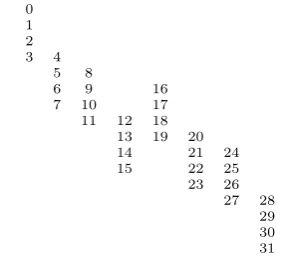
The edgeless graph for a given graph is obtained by re-moving all its edges, keeping its nodes at the same positions. In Fig. 3, the edgeless intrinsic order graph ofI5is depicted.
0 1 2
3 4
5 8
6 9 16
7 10 17
11 12 18
13 19 20
14 21 24
15 22 25
23 26 27 28
29 30 31
Fig. 3. The edgeless intrinsic order graph forn= 5.
For further theoretical properties and practical applications of the intrinsic order and the intrinsic order graph, we refer the reader to [5], [6], [7], [8], [9].
III. NEWPROPERTIES OF THEINTRINSICORDERGRAPH
When viewed as an undirected graph, the Hasse diagram is called the cover graph of the poset. We refer the reader to [1], for standard notation and terminology concerning graphs. Using Theorems 2.1, 2.2, and 2.3 we can derive many different properties of the cover graph ofIn. Here, we have
selected only a few of them.
A. Edges
LetVn andEn be the sets of vertices and edges,
respec-tively, ofIn. As usual,|A|denotes the cardinality of the set
A. As mentioned, the number of nodes of In is obviously
|Vn|=|{0,1} n
|= 2n.
Our first property gives the number of edges ofIn.
Proposition 3.1: For all n ≥ 1, the number of edges in the intrinsic order graphIn is
|En|= (n+ 1) 2n−2. (5)
Proof: The edges (going downward from u tov) in a Hasse diagram are exactly the covering relations (u B v). Hence, using Theorem 2.2, we obtain
|En|=|{(u, v)∈Vn×Vn |uBv}|
=|{(u, v)∈Vn×Vn |Mvu has the pattern (3)}|+
=|{(u, v)∈Vn×Vn |Mvu has the pattern (4)}|
=
u1 . . . un−1 0 u1 . . . un−1 1
+
=
u1 . . . ui−2 0 1 ui+1 . . . un
u1 . . . ui−2 1 0 ui+1 . . . un
[image:3.595.59.282.565.731.2]
as was to be shown.
Remark 3.1: Using proposition 3.1, we get for alln≥2
|En|= (n+ 1) 2n−2= 2·n·2n−3+2n−2= 2|En−1|+2n−2,
a recurrence relation for the number |En| of edges of In,
which could be also obtained directly from Theorem 2.2. When we use the binary representation, the set En of
all the (n+ 1) 2n−2 edges in In is given by Theorem 2.2.
The following proposition gives this set using the decimal numbering for the pairs of adjacent nodes (see Fig. 2).
Proposition 3.2: For alln≥1
En=
u(10, u(10 + 1
u(10 = 2p, 0≤p≤2n−1−1
[
n−2
[
m=0
u(10, u(10+ 2m
u(10 =q+ 2m(1 + 4r), 0≤q≤2m−1,
0≤r≤2(n−2)−m−1
.
Proof: The edges (going downward from uto v) in a Hasse diagram are exactly the covering relations (u B v). So, using Theorem 2.2, we obtain
En = u(10, v(10
∈Vn×Vn |uBv
= u(10, v(10∈Vn×Vn |Mvu has the pattern (3)
∪
u(10, v(10
∈Vn×Vn |Mvu has the pattern (4) .
On one hand, if Mu
v has the pattern (3) then we have that
v(10 =u(10+ 1, and
u(10 = (u1, . . . , un−1,0)(10
= 2 (u1, . . . , un−1)(10 = 2p 0≤p≤2
n−1−1
.
On the other hand, if Mu
v has the pattern (4) then making
the change of variable m=n−i, we get
v(10 =u(10+ 2n−i with2≤i≤n, i.e., v(10 =u(10+ 2mwith0≤m≤n−2and u(10 = (u1, . . . , ui−2,0,1, ui+1, . . . , un)(10
= (u1, . . . , ui−2,0,0,0, . . . ,0)(10 + (0, . . . ,0,0,1,0, . . . ,0)(10
+ (0, . . . ,0,0,0, ui+1, . . . , un)(10 = 2n−i+2(u1, . . . , ui−2)(10 + 2n−i+ (ui+1, . . . , un)(10
= 2m+2r+ 2m+q=q+ 2m(1 + 4r),
where, 0≤q≤2m−1 and0≤r≤2(n−2)−m−1.
Example 3.1: Letn= 4. Using Proposition 3.2, we get
A4=
u(10, u(10 + 1
u(10 = 2p,
0≤p≤2n−1−1 = 7
=
(0,1),(2,3),(4,5),(6,7), (8,9),(10,11),(12,13),(14,15)
,
B4= 2
[
m=0
u(10, u(10 + 2
m
u(10 =q+ 2m(1 + 4r),
0≤q≤2m−1, 0≤r≤22−m−1
=
(1,2),(5,6),(9,10),(13,14), (2,4),(3,5),(10,12),(11,13),
(4,8),(5,9),(6,10),(7,11)
,
where the three above rows respectively correspond to:
m= 0 : q= 0 r= 0,1,2,3 v(10 =u(10+ 20 m= 1 : q= 0,1 r= 0,1 v(10 =u(10+ 21 m= 2 : q= 0,1,2,3 r= 0 v(10 =u(10+ 22
Thus, E4 = A4∪B4 contains all the 20 edges (pairs of adjacent nodes) of the graphI4, as one can confirm looking at the right-most diagram in Fig. 2. Note that using (5) for
n= 4, we can also confirm that the cardinality of E4 is
|E4|= (n+ 1) 2n−2= 5·22= 20.
B. Shadows, Neighbors and Degrees
The neighbors of a given vertex u in a graph, are all those nodes adjacent to u (i.e., connected by one edge to
u). In particular, for (the cover graph of) a Hasse diagram, the neighbors of vertex ueither cover uor are covered by
u. This naturally leads to the following definition [10]. Definition 3.1: Let(P,≤)be a poset andu∈P. Then (i) The lower shadow ofuis the set
∆ (u) ={v∈P |v is covered byu}={v∈P |uBv}.
(ii) The upper shadow ofuis the set
∇(u) ={v∈P |v coversu}={v∈P |vBu}.
Particularly, for our poset P = In, regarding the lower
shadow ofu∈ {0,1}n, using Theorem 2.2, we have
∆ (u) ={v∈ {0,1}n |uBv}
={v∈ {0,1}n |Mvu has the pattern (3)} ∪ {v∈ {0,1}n |Mvu has the pattern (4)},
and hence, the cardinality of the lower shadow ofuis exactly
1−un (pattern (3)) plus the number of pairs of consecutive
bits(ui−1, ui) = (0,1) inu(pattern (4)). Formally:
|∆ (u)|= (1−un) + n
X
i=2
max{ui−ui−1, 0}. (6)
Similarly, for the upper shadow ofu∈ {0,1}n, using again Theorem 2.2, we have
∇(u) ={v∈ {0,1}n |vBu}
={v∈ {0,1}n |Muv has the pattern (3)}
∪ {v∈ {0,1}n |Muv has the pattern (4)},
and hence, the cardinality of the upper shadow ofuis exactly
un (pattern (3)) plus the number of pairs of consecutive bits
(ui−1, ui) = (1,0) inu(pattern (4)). Formally:
|∇(u)|=un+ n
X
i=2
max{ui−1−ui, 0}. (7)
Next proposition provides the total number of neighbors of each nodeuof the intrinsic order graphIn, the so-called
degree ofu, denoted, as usual, byδ(u).
Proposition 3.3: Letn≥1 andu∈ {0,1}n. The degree
δ(u)of u(i.e., the number of neighbors ofu) is
δ(u) = 1 +
n
X
i=2
Proof: Denoting by N(u) the set of neighbors of a vertexu∈ {0,1}n in the graph In, obviously we have
N(u) = ∆ (u)∪ ∇(u)
and from (6) and (7), we immediately obtain
δ(u) =|N(u)|=|∆ (u)|+|∇(u)|= 1 +
n
X
i=2
|ui−ui−1|,
as was to be shown.
Next proposition provides us with the set of neighbors of each node u of the intrinsic order graph In, using decimal
representation.
Proposition 3.4: Let n ≥ 1, and let u ∈ {0,1}n with Hamming weight m. Write u(10 as sum of powers of2, in
increasing order of the exponents, i.e.,
u(10 =
n
X
i=1
2n−iui= 2p1+ 2p2+· · ·+ 2pm (9)
(0≤p1< p2<· · ·< pm≤n−1).
(i) The lower shadow∆ (u)ofuis characterized as follows: (i)-(a) Ifu(10 is even (i.e., if un = 0) then
u(10+ 1∈∆ (u), i.e., u(10 . u(10+ 1.
(i)-(b) For any power 2p (0≤p≤n−2) in (9) s.t. 2p+1
does not appear in (9) then
u(10+ 2p∈∆ (u), i.e., u(10 . u(10+ 2p.
(ii) The upper shadow∇(u)ofuis characterized as follows: (ii)-(a) Ifu(10 is odd (i.e., if un = 1) then
u(10−1∈ ∇(u), i.e., u(10 −1. u(10.
(ii)-(b) For any power 2p (1≤p≤n−1) in (9) s.t. 2p−1
does not appear in (9) then
u(10 −2p−1∈ ∇(u), i.e., u(10 −2p−1. u(10.
Proof: The assertions (i)-(a) and (ii)-(a) immediately follow using pattern (3) in Theorem 2.2, for matrices Mu v
and Mv
u, respectively. The assertions (i)-(b) and (ii)-(b)
immediately follow using pattern (4) in Theorem 2.2, for matricesMu
v andMuv, respectively.
Example 3.2: Letn= 4 andu= (1,0,1,0). Then
u= (1,0,1,0)≡u(10 = 21+ 23= 10.
Using Proposition 3.4-(i), we get (note that u(10 = 10 is
even, i.e.,u4= 0)
∆ (10) ={10 + 1} ∪
10 + 21 ={11,12}
and using Proposition 3.4-(ii), we get
∇(10) =
10−20,10−22 ={6,9}.
Thus (see the graphI4, the right-most one in Fig. 2)
N(10) = ∆ (10)∪ ∇(10) ={6,9,11,12}
and using (8), we confirm that the cardinality ofN(10)is
δ(10) =|N(10)|= 1 + 4
X
i=2
|ui−ui−1| = 1 +|u2−u1|+|u3−u2|+|u4−u3| = 1 +|0−1|+|1−0|+|0−1|= 4.
C. Complementarity and Symmetry
Looking at any of the graphs in Figs. 2&3, we observe a “certain symmetry” in these diagrams. Let us formalize this fact.
Definition 3.2: Letn≥1 andu∈ {0,1}n.
(i) The complementaryn-tuple of uis then-tuple obtained by changing all its0s into1s and vice versa, i.e.,
(u1, . . . , un) c
= (1−u1, . . . ,1−un).
(ii) The complementary set of a subsetS ⊆ {0,1}n is the set of complementaryn-tuples of all the n-tuples ofS, i.e.,
Sc={uc |u∈S}.
Remark 3.2: Note that for all(u1, . . . , un)∈ {0,1} n
(u1, . . . , un) + (u1, . . . , un)c= (1, . . . ,1)≡2n−1.
Hence, the simplest way to verify that two binaryn-tuples are complementary, when we use their decimal representations, is to check that they sum up to2n−1. For instance, the binary
3-tuples 2 ≡(0,1,0) and5 ≡(1,0,1) are complementary, since2 + 5 = 7 = 23−1. Similarly, the complementary of
the binary 4-tuple 4 ≡(0,1,0,0) is 11≡(1,0,1,1), since
24−1
−4 = 15−4 = 11.
The reason underlying the symmetry of the intrinsic order graph is the duality property of the intrinsic order stated by the following proposition.
Proposition 3.5: Letn≥1 andu, v∈ {0,1}n. Then
u . v ⇔ vc. uc, uv ⇔ vcuc.
Proof: Clearly, the 00 , 11
, 01
and 10
columns in matrix Mvu, respectively become
1 1
, 00, 01 and 10 columns in matrixMvc
uc. Hence, using Theorem 2.2, we have
that u . v iff Mu
v has either the pattern (3) or the pattern
(4) iff Mvc
uc respectively has either the pattern (3) or the
pattern (4) iff vc . uc. Finally, the right-hand equivalence
immediately follows from the left-hand one and from the transitive property of the intrinsic order.
Many nice consequences can be derived from Proposition 3.5. Next corollary states only a few of them.
Corollary 3.1: Letn≥1. Letuandv be any two binary
n-tuples placed at symmetric positions (with respect to the central point) in the graphIn. Then
(i)uandvare complementaryn-tuples, i.e.,v=uc,u=vc.
(ii) The Hamming weights ofuandv sum up ton. (iii)∆ (u) =∇c(uc) =∇c(v), ∇(u) = ∆c(uc) = ∆c(v).
(iv) The sets of neighbors ofuandvare complementary. In particular,uandv have the same degree.
(v)u(10 is even (odd) ⇔v(10 is odd (even).
Proof:(i) It is a direct consequence of Proposition 3.5. (ii) It suffices to use (i) and the obvious fact that
wH(u) +wH(uc) =n.
(iii) Using Definition 3.1, Proposition 3.5 and (i), we get:
w∈∆ (u)⇔uBw⇔wcBuc⇔wc∈ ∇(uc) ⇔w∈ ∇c(uc)⇔w∈ ∇c(v)
and thus, taking complementaries, we get
∆ (u) =∇c(uc)⇒∆c(u) =∇(uc)
(iv) Using (iii), we get
N(u) = ∆ (u)∪ ∇(u) =∇c(v)∪∆c(v)
= [∇(v)∪∆ (v)]c=Nc(v)
and consequently
δ(u) =|N(u)|=|Nc(v)|=|N(v)|=δ(v).
(v) Using (i), we get
u(10 is even (odd) ⇔un= 0 (1)
⇔vn= 1 (0)⇔v(10 is odd (even)
and this concludes the proof.
Example 3.3: Letn= 4. The binary 4-tuplesu= 4and
v = 11 are placed at symmetric positions (with respect to the central point) in the graphI4 (see Fig. 2). Therefore:
(i) 4c≡(0,1,0,0)c = (1,0,1,1)≡11 4 + 11 = 24−1. (ii) wH(0,1,0,0) +wH(1,0,1,1) = 1 + 3 = 4 =n.
(iii)∆ (4) ={5,8}, ∇(11) ={7,10}, {5,8}c ={7,10}. ∇(4) ={2}, ∆ (11) ={13}, {2}c ={13}.
(iv) N(4) ={2,5,8},N(11) ={7,10,13},
{2,5,8}c={7,10,13} andδ(4) = 3 =δ(11). (v) 4 is even,11 is odd.
D. Isomorphic Subgraphs and Fractal Structure
A bisection of a graph is a partition of its vertex set into two (disjoint) subsets with half the vertices each [1]. The most natural way of bisecting the intrinsic order graph
In is the following. The first and second half, respectively,
of {0,1}n will be the subsets of binary n-tuples whose first component is u1 = 0 and u1 = 1, respectively. This
procedure can be reiterated by successively bisecting, in the same way, each of the so-obtained subgraphs.
Let n≥1,1 ≤k≤n and let u¯1, . . . ,u¯k ∈ {0,1} be k
fixed binary digits. From now on,Iu¯1,...,u¯k
n denotes the subset
of bitstrings of{0,1}nwhose first or left-mostkcomponents are fixed, namely u1 = ¯u1, . . . , uk = ¯uk; while its last or
right-mostn−kcomponents,uk+1, . . . , un, take all possible
values (0 or 1). More precisely, Iu¯1,...,u¯k
n is the set
n
(¯u1, . . . ,u¯k, uk+1, . . . , un)
(uk+1, . . . , un)∈ {0,1}
n−ko
and its cardinality is |I¯u1,...,u¯k
n |=
{0,1}
n−k
= 2
n−k.
Let us recall that two graphsG(V, E)andG∗(V∗, E∗)are said to be isomorphic if there exists an isomorphism of one of them to the other, i.e., an edge-preserving bijection [1]. That is, a graph isomorphism is a one-to-one mapping between the vertex setsΦ :V →V∗, which preserves adjacency, i.e.,
u, vare adjacent inGif and only ifΦ (u),Φ (v)are adjacent inG∗.
The self-similarity property or fractal structure that one can observe in Figs. 2&3, is an immediate consequence of the following proposition.
Proposition 3.6: Letn≥1and1≤k≤n. The2k equal-sized subgraphsIu¯1,...,u¯k
n (each with2
n−k nodes), obtained
after k successive bisections of the intrinsic order graph
In, are pair-wise isomorphic, and indeed all of them are
isomorphic to the intrinsic order graphIn−k.
Proof:Consider the following one-to-one mapping
Iu¯1,...,u¯k
n
Φ
−→ In−k
(¯u1, . . . ,u¯k, uk+1, . . . , un) 7−→ (uk+1, . . . , un)
Using Theorem 2.2, we have
(¯u1, . . . ,¯uk, uk+1, . . . , un).(¯u1, . . . ,u¯k, vk+1, . . . , vn)
if and only if
(uk+1, . . . , un).(vk+1, . . . , vn),
so thatΦis an isomorphism of graphs, since it preserves the edges (covering relations).
For instance, letn= 5andk= 3. Afterk= 3successive bisections of the intrinsic order graph I5, the 2k = 8
subgraphs are the8 isomorphic “columns” (each containing
2n−k= 4 nodes) depicted in Fig. 3. Moreover, any of these
“column”-subgraphs ofI5(5-tuples) is isomorphic toI2 (2
-tuples), the second graph from the left in Fig. 2.
IV. CONCLUSION
The behavior of a CSBS depends on the current values of the 2n binary n-tuple probabilities and on the ordering
between them. In this sense, the intrinsic order graph In
provides us with an useful representation of a CSBS, by displaying all the bitstrings in decreasing order of their occurrence probabilities. In this paper, several new properties of the digraph In have been stated and rigorously proved
(e.g., number of edges, neighbors and degrees of each vertex, symmetry, fractal structure, etc.). Each of these properties has been illustrated with a simple example and with the corresponding graph. Since many different technical systems in Reliability Engineering are indeed CSBSs, then our results can be applied to develop new (or to improve already known) algorithms –based on the intrinsic order– for evaluating the unavailability system. From a theoretical point of view, this paper suggests the search of new graph-theoretic and order-theoretic properties of the intrinsic order graphIn.
REFERENCES
[1] R. Diestel,Graph Theory, 3rd ed. New York: Springer, 2005. [2] L. Gonz´alez, “A New Method for Ordering Binary States Probabilities
in Reliability and Risk Analysis,”Lect Notes Comp Sc, vol. 2329, no. 1, pp. 137-146, 2010.
[3] L. Gonz´alez, “N-tuples of 0s and 1s: Necessary and Sufficient Condi-tions for Intrinsic Order,”Lect Notes Comp Sc, vol. 2667, no. 1, pp. 937-946, 2003.
[4] L. Gonz´alez, “A Picture for Complex Stochastic Boolean Systems: The Intrinsic Order Graph,”Lect Notes Comp Sc, vol. 3993, no. 3, pp. 305-312, 2006.
[5] L. Gonz´alez, “Algorithm comparing binary string probabilities in com-plex stochastic Boolean systems using intrinsic order graph,” Adv Complex Syst, vol. 10, no. Suppl. 1, pp. 111-143, 2007.
[6] L. Gonz´alez, “Complex Stochastic Boolean Systems: Generating and Counting the Binaryn-Tuples Intrinsically Less or Greater thanu,” in
Lecture Notes in Engineering and Computer Science: World Congress on Engineering and Computer Science 2009, pp. 195-200.
[7] L. Gonz´alez, “Partitioning the Intrinsic Order Graph for Complex Stochastic Boolean Systems,” in Lecture Notes in Engineering and Computer Science: World Congress on Engineering 2010, pp. 166-171. [8] L. Gonz´alez, “Ranking Intervals in Complex Stochastic Boolean Sys-tems Using Intrinsic Ordering,” in Machine Learning and Systems Engineering, Lecture Notes in Electrical Engineering, vol. 68, B. B. Rieger, M. A. Amouzegar, and S.-I. Ao, Eds. New York: Springer, 2010, pp. 397410.
[9] L. Gonz´alez, D. Garc´ıa, and B. Galv´an, “An Intrinsic Order Criterion to Evaluate Large, Complex Fault Trees,” IEEE Trans on Reliability, vol. 53, no. 3, pp. 297-305, 2004.