Low Flow Trends and Frequency Analysis in the Blue Nile Basin, Ethiopia

http://www.scirp.org/journal/jwarp ISSN Online: 1945-3108

ISSN Print: 1945-3094

DOI: 10.4236/jwarp.2018.102011 Feb. 28, 2018 182 Journal of Water Resource and Protection

Low Flow Trends and Frequency Analysis in

the Blue Nile Basin, Ethiopia

Kidist Assefa

_{, Mamaru A. Moges}

1_{Amhara Water Irrigation and Energy Bureau, Bahir Dar, Ethiopia}

2_{Faculty Civil and Water Resources Engineering, Bahir Dar Institute of Technology, Bahir Dar University, Bahir Dar, Ethiopia}

3_{Blue Nile Water Institute, Bahir Dar University, Bahir Dar, Ethiopia}

Abstract

Low flow analysis provides crucial information for the planning and design water resource development, risk assessment and environmental flow man-agement. Understanding the low flow regimes and evaluating the magnitudes for incorporating in water resources management is vital for the countries like Ethiopia where demand for water is increasing. However, there were hardly enough studies in understanding the trends of low flow and frequency analy-sis. Therefore, this study focuses on evaluation of the trends in low flows and regional low flow analysis in the Blue Nile Basin, Ethiopia. In order to carry out the study, 15 river sub-basins in the Blue Nile Basin were selected based on the long term data availability and presence of quality of data. The 3-day sustained low flow (3d-slf), the 7-day sustained low flow (7d-slf) and the 14-day sustained low flow (14d-slf) models were used to extract the data from the daily time series stream data obtained from MoWIE. Trends in low flow were analyzed separately by using Mann-Kendall (MK) trend test. Low flow frequency analysis was used to estimate the long term low flow quantiles. In addition, regional analysis for estimating the quantiles for ungaged catch-ments was also developed based on the regional growth curve and catchment characteristic of drainage basins. The results indicated that 3d-slf, 7d-slf and 14d-slf models of low flow series indicated no significant difference for each station at 95% CI. Out of the 15 selected stations, 12 of stations have indicated decreasing; two stations indicated increasing and remaining one station with no trend. Mainly decreasing trend was associated with the land cover and cli-mate change which results in increasing runoff and evapotranspiration re-spectively. Weibull distribution—GEV and LGN was found best fit based on the L-Moment Ratio Diagram (L-MRD). Hence quantile estimations have in-dicated diminishing magnitudes of low flow quintiles for 2 - 500 years return

How to cite this paper: Assefa, K. and Moges, M.A. (2018) Low Flow Trends and Frequency Analysis in the Blue Nile Basin, Ethiopia. Journal of Water Resource and Protection, 10, 182-203.

https://doi.org/10.4236/jwarp.2018.102011

Received: January 26, 2018 Accepted: February 25, 2018 Published: February 28, 2018

Copyright © 2018 by authors and Scientific Research Publishing Inc. This work is licensed under the Creative Commons Attribution International License (CC BY 4.0).

DOI: 10.4236/jwarp.2018.102011 183 Journal of Water Resource and Protection

periods. Regional low frequency analysis has provided a very good relation-ship between discharge and catchment characteristics with an R2 _{of 0.72.}

Where area (A) and rainfall (R) followed by slope were found sensitive to compute in developing the regional region equations between mean low flows and the physiographic data. This study indicated that there needs to be a new water management scenario and adaptation mechanism of climate change and land use land cover dynamics for utilizing water resource in the Blue Nile Basin.

Keywords

Mann-Kendall, Low Flow, L-MRD, PWM, Regionalization, Blue Nile Basin

1. Introduction

Low flow is the smallest sustained average daily flow rate or volume with time

[1]. It is an important part of the natural flow regime of rivers where the water resource planning and design consider its spatial and temporal variability. Low flow analysis is important for basin management, river abstraction, effluent dilu-tion, navigation purposes, ecosystem protection and environmental flow limit

[2].Sometimes it uses as an indicator of hydrological drought during the conti-nuous low-flow period in one year [3]. According to [2] low flow information is needed in three situational cases 1) for water resource development, 2) to ex-ecute the daily decisions on managing the water resource development during operational phases, and 3) when there is a current need to decide on the opera-tions based on the estimaopera-tions of the future stream flows. Nevertheless, very of-ten in most part of the rivers the low flows are indicating signs of decreasing flow rate and volume.

Decreasing in low flow would impact the environmental flow in a given eco-system and affect multi-purpose operations which depend on that water eco-system such as river and lakes. It could happen due to different ways, for instance groundwater pumping close to the head of a perennial river during the dry sea-son [4], due to the dynamics in vegetation cover as a result of deforestation [5], due to the an expansion of irrigation which requires withdrawal of water from rivers in dry seasons [6]. Reduced low flow may also cause an impairment of water quality, and affect river ecological status and navigation and power supply sectors [7]. To understand the causes and take remedial action for the sustaina-ble utilization of the low flows the dynamics in low flows in a river system should be evaluated, which could include quantifying the trend of low flow quantiles, and developing regional curves (ungaged catchments) is a very im-portant approach for proper management of the water resources.

geo-DOI: 10.4236/jwarp.2018.102011 184 Journal of Water Resource and Protection

graphical regions and to variations in upstream sub-basin characteristics. Low flow frequency analysis and predictions generally have to deal with the inade-quacy or deficiency of observations for the site of interest [8]. Information for an ungaged site may be obtained either by means of deterministic models or by re-gionalization techniques based on available observed flow records from gauged stations.

In the Blue Nile Basin an increase in population over the past few years has put great pressure on the natural resources, where it has led to increase in de-mand for more water and agricultural land and resulting deforestation [9][10] [11]. In the under this study, recently there are observations on drying out of some rivers, where the low flow is becoming no flows. However there have not been many studies carried out especially in evaluating trends and estimation technique for long term quintiles of low flow. Hence understanding the low flow trends and develop estimation techniques for ungaged catchments is paramount. In addition evaluation of low flow is important for water resource development and management for sustainable and proper utilization of water resource and maintaining the environmental flows. Therefore this study presents trends and frequency analysis of the low flow in the selected rivers in the Blue Nile Basin, Ethiopia. In addition regional low flow analysis to estimate the low flow quan-tiles from the ungaged catchments was also carried out in this study.

2. Materials and Methods

2.1. Description of the Study Area

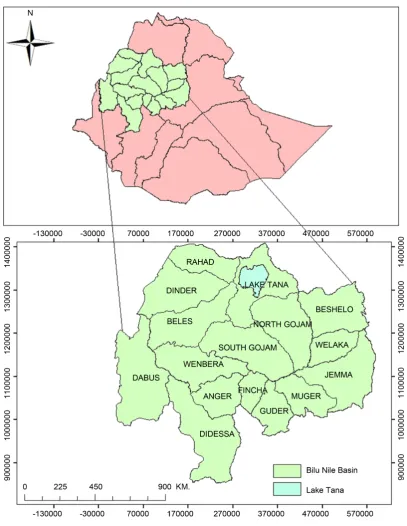
The Upper Blue Nile River “Abbay” basin (Figure 1) lies in the western part of Ethiopia between latitudes of 7˚45'N and 12˚46'N and longitudes of 34˚05'E and 39˚45'E. The basin has an estimated area of 199,812 km2_{. The basin covers 17%}

land area of the country and lies in three national regional states where 46% of the basin area is Amhara, 32% in Oromia and 22% in Binishangul-Gumuz. It Locally the climate in the basin is subdivide as the dry season “Bega” from Oc-tober to the end of February; the short rain period “Belg” from March to May and the long rainy period “Kiremt” from June to September, highest amount of rainfall in July and August. The average annual rainfall ranges from 1200 mm/year - 1800 mm/year [12]. The rivers flow in the basin was described by the rainfall variability [13]. The 100 year mean annual flow volume of the Blue Nile river (monitored at El Diem) was nearly 50 Bm3 [14] where 8% flow volume was observed at Bahir Dar (at Cherechra gaging station) and 32.9% was at Kessie

[12]. Annual stream flow variability in the basin ranges up to maximum of 20%

DOI: 10.4236/jwarp.2018.102011 185 Journal of Water Resource and Protection Figure 1. Location map of the study area.

basic rocks (dominantly basalts) and the lowland part near the Sudanese border was composed of basement complex rocks and metamorphic rocks [17].

2.2. Methodology

DOI: 10.4236/jwarp.2018.102011 186 Journal of Water Resource and Protection

3) low frequency analysis for selected station in the basin and 4) regionalization of the low flow for estimating the quantiles for the ungaged catchments.

2.2.1. Data Availability

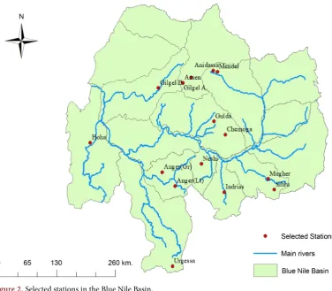
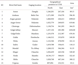
Data needed for this study were collected from different organization in order to use for low flow trends, frequency and regional frequency analysis. Limited record length was typically a major challenge interpret the results of trend analy-sis, as there are often few homogeneous records on which the statistical analysis could be carried out. The stream flow data used for the low flow analysis was obtained from the Ministry of Water Irrigation and Electricity (MoWIE). Among the functional stream flow stations in the basin 15 river gaging stations (Figure 2, Table 1) were selected. The selection was based on 1) the long record of data, less missing records and functionality and 2) consideration of the spatial distributions of gaging stations and sub basins in the basin. Duration of data availability for the low-flow analysis used for this study ranged with 10 to 42 years of record length. The missing data in the daily stream flow was carried out based on the extent of missing data. Station-average method (for missing data less 10%) and normal ratio method (missing data higher than 10%) has been used [18] to infill the missed data. The low flow data extraction was based on the 3 day sustained low flow (3d-slf), the 7 day sustained low flow (7d-slf) and the 14 day sustained low flow (14d-slf) for the selected stations.

DOI: 10.4236/jwarp.2018.102011 187 Journal of Water Resource and Protection Table 1. Data availability and source for the selection of stations.

ID River/Sub basin Gaging location

Geographical

position in UTM Area

North East km2

1 Amen Dangila 1,246,201 267,104 89.15

2 Andassa Bahir Dar 1,271,589 334,578 596.38

3 Angar-greater Nekemte 1,060,930 220,413 1099.03

4 Angar-lower Nekemte 1,032,779 249,835 619.66

5 Chemoga Debremarkos 1,138,754 361,295 364.25

6 Gelgel abbay Marawi 1,257,136 285,380 1656.00

7 Gelgel beles Mandura 1,235,578 212,387 676.56

8 Gulda Dembecha 1,166,512 335,870 249.28

9 Hoha Asossa 1,122,346 678,950 161.12

10 Indris Guder 1,019,788 358,631 118.13

11 Mendel Tis Abbay 1,268,152 364,364 91.35

12 Muger Chancho 1,056,459 443,536 549.49

13 Neshi Shambo 10,781,717 308,031 322.43

14 Sibilu Chancho 1,028,748 467,164 380.12

15 Urgessa Gembe 897,894 232,531 19.11

2.2.2. Trends in Low Flow

Evaluating the presence and absence of trends in low flow for the selected sta-tions was carried out by using the Mann and Kendall (MK) trend test [19]. MK trend test (Equations (1)-(3)) evaluates and indicates the absence and presence of the monotonic increasing/decreasing trend. MK trend test was a non-parametric rank-based [12] method which was widely used to test the randomness against trend in hydro-climatologically time series data [20]. The existence of trend was explained as no trend, increasing trend and decreasing trend based on the signi-ficance level of test static [21]. It does not require assumptions about the statis-tical distribution of the data. The test statistic, S (Equation (1)) calculates as the sum of the difference between data points and the associations between samples which is referred as Kendal tau to show the presence or absence of trend. A posi-tive value of S indicates an increasing trend while a negative value shows a de-creasing trend [22].

(

)

1

1 1

sgn

n n

j i

i j i

S x x

−

= = +

=

∑ ∑

where xj and xiare the daily values in days’ j and i, j > i, respectively and

(

)

sgn 0 if 0

1 if 0

j i

j i j i

j i

x x

x x x x

x x

 − >



− = − =

− − <



If n < 10, the value of |S| is compared directly to the theoretical distribution of

DOI: 10.4236/jwarp.2018.102011 188 Journal of Water Resource and Protection

( )

( )

if 0

0 if 0

1 if 0 S S S V S Z S S S V S −  _>    =_ =  ₊  <  (2)

The MK trend test ZS statistics (Equation (2)) determines the presence of

de-creasing or inde-creasing trend if is negative and positive respectively. The test sta-tistic ZS is also used a measure of significance of trend. If |Zs| is greater than Zα/2,

where α represents the chosen significance level (e.g.: 5% with Z0.025 = 1.96)

im-plying that the trend is significant [23] and V(S), the variance of statistic was given as in Equation (3).

( )

(

)(

)

(

)(

)

1 2 5 1 2 5

m

i i i

t

n n n t t t

V S

N

=

− + − − −

=

∑

2.2.3. Low Frequency Analysis

The purpose of low frequency analysis in this study was to estimate the long term quantiles of for different return periods and regionalize estimations in or-der to compute the low flows for ungaged estimates. Detail procedure of the frequency analysis used in this study was presented as follows.

1) Selection of low flow models

The K days sustained low flow method of data extracting was used to prepare the data for low flow trends and frequency analysis for the selected stations. Where the lowest K day’s stream flow data per year has been averaged to obtain k days sustained (mean) low flow (Kd-slf) as presented in equation 4. Three dif-ferent models have been used for selecting the low flow data series for this study including the three days-sustained low flow (3d-slf) model, the seven days-sustained low flow (7d-slf) model and the fourteen days sustained low flow (14d-slf) model. 2 Kd-slf n i i n x K = −

=

∑

where K is the number of sustained days, n is the number of data in time series (365 and 366 in leap years) and Xi the daily time series of stream flow (m3/s)

2) Data quality analysis

DOI: 10.4236/jwarp.2018.102011 189 Journal of Water Resource and Protection

3) L-moments

[27] stated that the L-moments as the summary statistics for probability dis-tributions and data samples. Which are analogous to ordinary moments and provide measures of location, dispersion, skewness, kurtosis, and other aspects of the shape of probability distributions or data, where these are computed from linear combinations of the ordered data. It`s properties hold in a wide range of practical situations [27]. For instance the asymptotic approximations for sam-pling distributions are better for L-moments than the ordinary moments. It also provides better identification of the parent distribution generated by a particular data sample. L-moments can characterize a wider range of distributions, com-pared to the conventional moments. For this study the L-moments have been used for selecting the best fit probability distribution and during parameter es-timation for each station.

4) Selection probability distribution a) L-Moment Ratio Diagram (L-MRD)

One of the main applications of L-moments is identification of the probability distribution of the observed phenomena using the L-MRD. This was based on relationships between the L-moment ratios [28]. A theoretical diagram based on

L-Cs (τ3) versus L-Ck (τ4), was used similar to the conventional MRDs to

identi-fy appropriate distributions. For a given region, the sample L-moment ratios τ3

and τ4 for each station as well as their regional average are plotted on the

L-moment ratio diagram. A suitable parent probability distribution was identi-fied which averages the scattered data and around which the data spread consis-tently. For this study the L-moments were used to identify the parent probability distributions. Since the L-MRD was based on unbiased sample quantities which have to be corrected for bias. L-MRD plot as fairly well separated groups and permit better discrimination between the distributions.

5) Selection of parameter estimation method

After selecting the best fit probability distribution for each station the para-meters of probability distribution could be estimated in a number of estimation techniques. Some of methods of parameter estimation [28] indicated the most commonly used parameter estimation methods were a) Method of Moments (MOM), b) The Maximum Likelihood Method (MLM), c) The Probability Weighted Moments (PWM) methods. For this study Probability Weighted Mo-ment (PWM) [29] method of parameter estimation was chosen due to its appli-cability and ease of implementing for regional parameter and quantile estima-tion [28]. The method was often defined by plotting position estimates of M1,o,s

and M1,r,0 in Equations (5)-(6).

(

)

1, , 1

1

1 s

N

s s o s i i

a M F X

N

α ₌

= = = =

∑

1, ,0 1

1 N r

r r r i i

b M Fi X

N

β ₌

= = = =

∑

DOI: 10.4236/jwarp.2018.102011 190 Journal of Water Resource and Protection

0 0

α =β β0=α0

1 0 1

α =β −β β α₁= ₀−α₁

2 0 2 1 2

α =β − β β+ β2=α0−2α α1+ 2

3 0 3 1 3 2 3

α =β − β + β −β β₃=α₀−3α₁+3α α₂− ₃

F in Equations (5)-(6) can be estimated from the plotting position formulas among the many for this specific study it was estimated by [27]as indicated in Equation (7). 1 2 i a N F a − + −

= ₍₇₎

Hosking (1986 and 1990) indicated the L-moments, which are linear functions of PWMs and defined in terms of the PWMs α and β by Equations (8)-(11)

1 0 0

l =α =β (8)

2 0 2 1 2 1 0

l =α − α = β β− (9)

3 0 6 1 6 2 6 2 6 1 0

l =α − α + α = β − β β+ (10)

4 0 12 1 30 2 20 2 20 3 30 2 12 1 0

l =α − α + α − α = β − β + β β− (11)

where the ratio of L-moments (τr) used in this study were analogous to

conven-tional moment ratios as defined by [27] as indicated in Equations (12) and (13)

2

1

l l

τ = ₍₁₂₎

1

r r

l l

τ = for r≥3 (13)

where ll is a measure of location, τ is a measure of scale and dispersion (LCv), τ3

is a measure of skewness (LCs), and τ4 is a measure of kurtosis (LCk) defined by

Equations (14)-(16)

L-Coefficient of variation (LCv) = 2 1

l l

τ = ₍₁₄₎

L-Coefficient of skewness (LCs) = 3 3

2

l l

τ = ₍₁₅₎

L-Coefficient of kurtosis (LCk) = 4 4

2

l l

τ = ₍₁₆₎

6) Quantile estimation of low flows

The estimated parameters for specific probability distributions were used to calculate quantiles of low flows for different return periods. This was carried out by using the distribution function, in which the parameters of the distribution were replaced by their estimates and the relationship between return periods (T) and probability of exceedance (F). In low flow frequency analysis the assumption for the relationship between the low flows quantiles with return period was based on the exceedance probability as indicated in Equation (17).

1

F T

DOI: 10.4236/jwarp.2018.102011 191 Journal of Water Resource and Protection

where F is the probability distribution function and T is the return period

2.3.4. Regional Low Flows for Ungaged Catchments

In order to carry out the regional low flow analysis initially the homogeneous group of stations has to be identified and categorized by using the L-MRD and coefficient of variation of coefficient of variation (C-C) test. The station year method was used for estimating the standardized long term quantiles for devel-oping the regional frequency curve. The station year methods pull the standar-dized low flow values as one station for each homogenous group. The best probability distribution for each homogenous group (pulled standardized data) was fit by using similar to procedures as discussed in above sections. Using this probability distribution, the long term standardized quantiles was estimated for various return periods such as 2, 10, 25, 50, 100, 200 and 500 years. The regional growth curve was established as the relationship between the standardized quan-tiles and return periods for each return period. Hence the estimated standar-dized quantile was used to compute the normal low flow quantiles for both gaged and ungaged stations was using the relationship under Equation (18).

*

T T

Q =Q X (18)

where QTis the low flow for T-years of return period, Q is the n-day sustained

average annual low flow, XT standardized quantile of for T years return period.

To compute the low flow quantiles for ungaged catchment using equation 18, the relationship between the n-day sustained average annual low flow of gaged stations and physical catchment characteristics has to be set up. Developing the relationship between the sustained average annual low flow and the catchment characteristics was also used for predicting the low flow quantiles at any point where the regional frequency curve was derived. In order to carry out the pre-diction, there are a number of measurable physical characteristics of catchments that could have significant relationship with the n-day sustained average low flow. Several physical catchment characteristics have been used for developing models to simulate the n-day sustained annual low flows for the ungaged catch-ments. The non-linear regression (Equation (19)) was used to develop a rela-tionship between the average annual low flow for ungaged catchments in Blue Nile River basin. For this study the mainly used(easily measurable) physical cat-chment characteristics such as area (A), rainfall (R), slope (S), stream length (L) and shape factor (F) was considered as independent variables.

a s r t t

Q=CA S R L F (19)

where Q is the average n day sustained low flow each station, A is the drainage

of the selected station in square kilometers, S is average Slope expressed in per-centage, R is the mean annual rainfall in millimeters, L is the length of stream, F

DOI: 10.4236/jwarp.2018.102011 192 Journal of Water Resource and Protection

3. Results and Discussion

3.1. Data Analysis and Quality

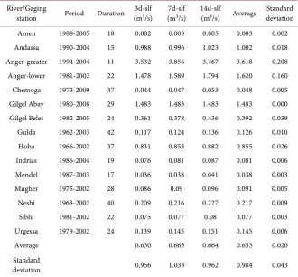
The three low flow data extraction models (3d-slf, 7d-slf and 14d-slf) in the se-lected 15 stations have been summarized and presented in Table 2. Descriptive statistics of low flow data was presented in Table 2. The maximum low flow has been observed in Anger-greater station with an average 3.61 m3_{/sec and the}

low-est observation in Amen station with 0.003 m3_{/sec. The standard deviation of the}

average of the low flow models provided 0.71 with maximum observed 3.01 at Anger-greater station and the minimum at Amen station with standard devia-tion of 0.0013. The results of low flow data series selecdevia-tion using the 3d-slf, 7d-slf and 14d-slf has indicated in-significant variation based on the ANOVA (Table 3) analysis for all of the stations under this study. Hence the averages of the three data selection models have been used for trends and frequency analysis.

Table 2. Low flows for the selected stations in the Blue Nile Basin.

River/Gaging

station Period Duration 3d-slf (m³/s) (m³/s) 7d-slf 14d-slf (m³/s) Average Standard deviation

Amen 1988-2005 18 0.002 0.003 0.005 0.003 0.002

Andassa 1990-2004 15 0.988 0.996 1.023 1.002 0.018

Anger-greater 1994-2004 11 3.532 3.856 3.467 3.618 0.208

Anger-lower 1981-2002 22 1.478 1.589 1.794 1.620 0.160

Chemoga 1973-2009 37 0.044 0.047 0.053 0.048 0.005

Gilgel Abay 1980-2008 29 1.483 1.483 1.483 1.483 0.000

Gilgel Beles 1982-2005 24 0.361 0.378 0.436 0.392 0.039

Gulda 1962-2003 42 0.117 0.124 0.136 0.126 0.010

Hoha 1966-2002 37 0.831 0.853 0.882 0.855 0.026

Indrias 1986-2004 19 0.076 0.081 0.087 0.081 0.006

Mendel 1987-2003 17 0.036 0.038 0.041 0.038 0.003

Mugher 1975-2002 28 0.086 0.09 0.096 0.091 0.005

Neshi 1963-2002 40 0.209 0.216 0.227 0.217 0.009

Siblu 1981-2002 22 0.075 0.077 0.08 0.077 0.003

Urgessa 1979-2002 24 0.139 0.145 0.151 0.145 0.006

Average 0.630 0.665 0.664 0.653 0.020

Standard

deviation 0.956 1.033 0.962 0.984 0.043

Table 3. ANOVA for 3d-slf, 7d-slf and 14d-slf data for the selected stations.

Source of

Variation SS dof MS F P-value F-crit

Between Groups 0.077813 2 0.039 0.015 0.98 3.22

Within Groups 105.402 42 2.51

DOI: 10.4236/jwarp.2018.102011 193 Journal of Water Resource and Protection

The outliers found from the low flow data tie series were very few in numbers and was decided and was removed before further analysis. From all of the sta-tions there were not higher outlier greater than the upper bound and the fewer existing ones in four stations were below the lower bound. Where one lowest outliers were found from the stations of Anger-lower, Hoha, Mendel and Neshi stations. The minimum of sustained low flow value’s in Anger-lower data series was 0.03 m3_{/s (in 1983) which was far below the lower outlier (X}

L) bound

(0.08358 m3_{/s). In Hoha station sustained low flow (0.001 m}3_{/s) recorded in 1978}

was lower than the outlier (XL) bounds (0.00273 m3/s). Similarly in Mendel

sta-tion the minimum sustained low flow was 0.0017 m3_{/s recorded in 2003, which}

was lower than the lower outlier (XL) bound (0.0023 m3/sec). In Neshi station XL

the lowest low flow value was 0.049 m3_{/sec observed in the year of 1981 lower}

than the lower outlier (XL) bound (0.056 m3/s). Hence these values were

re-moved from the data series of each station.

An independence test where the assumption in the use of statistical distribu-tion for extreme flow analysis of the sample data should be random without any serial correlation. It helps describes the strength of the relationship between a value in a series and that preceding it by one-time interval. Based on the W-W test all the selected stations sustained low flow data series was found indepen-dent. Hence the data series was accepted for the trend and frequency analysis of the low flows. All of the selected stations low flow data series were not stationary and homogenous except one station namely Gilgel Belles which likely could be the presence of trends.

3.2. Low Flow Trend Analysis Results

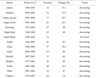
The trend test on low flow for the selected stations were carried out by using the Mann-Kendall (MK) test as discussed in the methodology section. As presented in Table 4 and Table 5 nearly 12 of the selected station shave indicated decreas-ing trend s of low flows. The decrement change of the low flows ranges from the selected stations range from 24.1% in Angar-great and extend to the maximum in 85% in Gulda stations. Two of the stations (Angar_lower and Hoha) from the selected stations have indicated an increasing trend with the positive change of low flow values of 43.3% and 10.1% (Figure 3). Unlike the other stations Gilgel Belles station has also indicated no significant trend.

There could be several reasons for decreasing of low flows in the Blue Nile Ba-sin. Some of this includes change in physical characteristics of catchment such as the land cover change in rivers basins. For instance, the change of the forest to agricultural land could largely increase runoff in the rainy season and reduce the low flows in dry seasons. This has been indicated in some of the Blue Nile Basin in different studies such as [30] land cover change in three micro watersheds (Ene-chilala, DebreMawi and Mizwa) in the Blue Nile Basin indicated that the land cover change from forest to Agriculture was 36% from 1973 to 2013. [31]

DOI: 10.4236/jwarp.2018.102011 194 Journal of Water Resource and Protection Table 4. Summary statics of the Mann-Kendall trend test for the 7d-slf trend analysis with α = 0.05.

River/Gaging

station Kendall’s tau S Var(S) (two-tailed) p-value Sen’s Slope

Amen −0.494 −38 266.67 0.023 −2E−4

Andassa −0.559 −50 330.00 0.007 −0.033

Anger-greater −0.556 −25 0.00 0.029 −1.584

Anger-lower 0.595 91 0.00 0.000 0.288

Chemoga −0.513 −40 0.00 0.015 −0.007

Gilgel Abay −0.604 −180 1829.33 0.0001 −0.062

Gilgel Belles 0.336 85 0.00 0.026 0.023

Gulda −0.566 −397 6325.00 0.0001 −0.005

Hoha 0.322 203 5389.00 0.006 0.006

Indrias −0.446 −68 696.00 0.011 −0.007

Mendel −0.433 −52 0.00 0.020 −0.003

Mugher −0.275 −95 2289.67 0.049 −0.003

Neshi −0.744 −58 0.00 0.000 −0.024

Siblu −0.418 −84 1064.67 0.011 −0.002

Urgessa 0.325 68 1094.67 0.043 0.003

Table 5. Trends in the low flow for the selected stations in the Blue Nile Basin.

Station Period (G.C) Duration Change (%) Trend

Amen 1988-2005 18 57.1 decreasing

Andassa 1990-2004 15 33.3 decreasing

Anger_greater 1994-2004 11 24.1 decreasing

Anger_lower 1981-2002 22 43.3 Increasing

Chemoga 1973-2009 37 98 decreasing

Gilgel Abay 1980-2008 29 68 decreasing

Gilgel Belles 1982-2005 24 - No trend

Gulda 1962-2003 42 85 decreasing

Hoha 1966-2002 37 10.1 Increasing

Indris 1986-2004 19 80 decreasing

Mendel 1987-2003 17 60 decreasing

Mugher 1975-2002 28 60 decreasing

Neshi 1963-2002 40 72.5 decreasing

Siblu 1981-2002 22 47 decreasing

Urgessa 1979-2002 24 78 decreasing

DOI: 10.4236/jwarp.2018.102011 196 Journal of Water Resource and Protection Figure 3. Trends in the 7d-slf from the river stations (a)-(o).

Basin). [32] estimated the change in land cover from forest to agricultural and from 1973 to 2005 by 43.2% and indicated a decrease in low flows during this time period [33] 1957 to 1995 in the Dembecha (part of upper Blue Nile Basin) area with decrease in forest cover from 27% in 1957 to 2% in 1982 and to 0.3% in 1995. In general, the change in land cover and poor agricultural practices in-creased the runoff and were one of the causes in reducing reduction the base flow and ultimately the lowest sustained low flows in the rivers of the Blue Nile which supports most of the results found in this study.

In addition, climate change could also be responsible due to an increasing temperature in the region which increases open water and soil water evapora-tion. This reduces the low flow to go down due to decrease of soil water in the ground water due to increasing evaporation. In Blue Nile Basin there were sev-eral sub basin specific studies which indicated an increase in trends of tempera-ture causing an increasing evapotranspiration such studies include National Meteorological Agency [34] and [35] in the Blue Nile Basin [36] and [37] over Lake Tana basin, [38] and [39] in Gilgel Abay watershed and [40] in the upper Blue Nile Basin.

3.3. Low Flow Frequency Analysis

DOI: 10.4236/jwarp.2018.102011 197 Journal of Water Resource and Protection 3.3.1. L-Moment Ratio Diagrams

For this specific study the moment ratio diagrams were used for two purposes 1) to identify the best fit probability distribution for each station and 2) to select homogeneous regions based on the best fit probability distributions and statis-tical tests for regionalization purpose. Based on the results from the L-MRD (Figure 4) from the selected 15 stations it was found that 10 stations were fitted with Weibul probability distribution for 7d-slf data. The stations were Amen, An-ger-greater, Anger-lower, Gilgel Beles, Gilgel Abay, Indrias, Mendel Neshi and Urgessa. Similarly, Andassa and Gudla stations were best fit with Log normal probability distributions. Hora, Mugher and Chemoga river stations were best fit for General Parent probability distributions (Table 6).

Figure 4. L-MRD for the selected flow gaging stations in the Blue Nile Basin.

Table 6. Probability distributions for the selected stations used in this study.

Stations Probability distribution

Amen Weibull

Andassa Log Normal (LGN)

Anger (Gr) Weibull

Anger (Lt) Weibull

Chemoga Generalized Extreme Value (GEV)

Gilgel Abay Weibull

Gilgel Beles Weibull

Gulda Log Normal (LGN)

Hoha Generalized Extreme Value (GEV)

Indrias Weibull

Mendel Weibull

Mugher Generalized Extreme Value (GEV)

Neshi Weibull

Siblu Weibull

Urgessa Weibull

0 4 8 12 16 20

0 0.5 1 1.5 2

L

_

Ck

L_Cs

GPAR

GLOG

GEV

P(3)

LOGN

Weibull

DOI: 10.4236/jwarp.2018.102011 198 Journal of Water Resource and Protection 3.3.2. Parameter Estimation

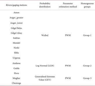
As discussed in the methodology section the parameter for the selected probabil-ity distributions, parameter has been estimated by using the PWM as summa-rized in Table 7. For all of the selected stations under for three groups of proba-bility distributions the Probaproba-bility Weighted Moment was used to estimate the parameters for computing the quantiles. Where 10 of the stations were fitted Weibull probability distribution while the reaming 2 and 3 stations with LNG and GEV with group 2 and 3 respectively (Table 7) as group of homogenous region.

Table 7. Low flow best fit probability distributions with parameter estimation techniques.

Rivers/gaging stations _distribution Probability _{estimation method} Parameter Homogenous _groups

Amen

Weibul PWM Group-1

Anger_greater Anger_lower

Gilgel Beles Gilgel Abay Indrias Mendel Neshi

Siblu Urgessa Andassa

Log Normal (LGN) PWM Group-2

Gulda Hora

Generalized Extreme

Value (GEV) PWM Group-3

Mugher Chemoga

3.3.3. Quintiles Estimations

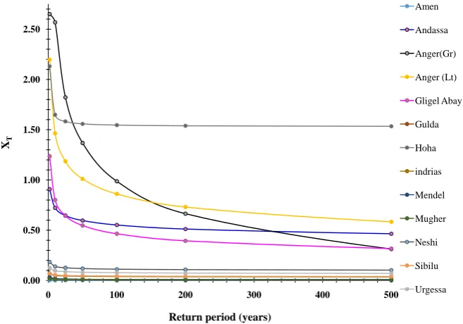
DOI: 10.4236/jwarp.2018.102011 199 Journal of Water Resource and Protection Figure 5. Quantile estimation of 7d-slf for the selected station in the Blue Nile Basin.

3.4. Regional Low Flow Analysis

The first step in regionalization was identifying the homogeneous regions or clustering based on different techniques. In this study the moment ratio diagram specifically the L-MRD was used for identifying the homogeneous groups. In addition the Coefficient of Variation of Coefficient of Variation (C-C) test was also carried out to further verify the homogenous regions. Based on the results from the L-MRD and CC based test the homogeneous regions were categorized as indicated in Table 8, where 10 stations were assigned as homogenous region group-1 with Weibull as the best fit probability distribution. While the remain-ing 2 and 3 stations assigned homogenous groups 2 and 3 with Log Normal (LGN) and Generalized Extreme Value (GEV) as the best fit probability distri-bution. Based on each homogenous group and best fit probability distribution the regional low flow curve equations to quantify the standardized quantiles of each group are provided in Table 8. Hence the regional standardized equations could be used for estimating standardized quantile for any ungaged site in the homogenous region and further to estimate the stream flow quantiles from the catchment characteristics derived average stream flow.

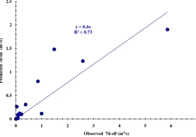
Using the catchment characteristics as in order to drive the low flows the best fit nonlinear regression was established. The relation between the predicted and observed low flows indicated a good predicting capability with an R2 _{of 0.73}

(Figure 6). The sensitive parameters during calibration of non-linear regression equation were area of drainage basins and rainfall sequentially followed by slope of the watershed. Hence using the regional growth curves under Table 8 and Equa-tion (20)could help to estimate long term quantiles for ungaged catchment.

1.0412 0.013 1.089 0.074

0.201

Q= A S− R− F (20)

0.00 0.50 1.00 1.50 2.00 2.50

0 100 200 300 400 500

XT

Return period (years)

DOI: 10.4236/jwarp.2018.102011 200 Journal of Water Resource and Protection Figure 6. Predicted and observed 7d-slf using catchment characteristics.

Table 8. Summary of regional growth curve equation.

Stations Probability Best fit distribution

Regional low flow Growth curve equations.

Amen

Weibull

( )

0.059 1.039 log 1

T

Q = + _ T _

Anger_Great Anger_Lower Gilgel Beles Gilgel Abay Indrias Mendel Neshi

Siblu Urgessa Andassa

Log Normal (LGN)

(

)

0.073 0.653 1 log1

T

Q = + _ − − T _

Gulda Hoha

Generalized Extreme Value (GEV)

0.33 0.468

e U

T

Q = +

Mugher Chemoga

4. Conclusion

The results in this study have indicated mainly a decrease in low flows values for the selected stations in the Blue Nile Basin. This was attributed to the catchment dynamics especially land cover change and climate change over the river basins. In addition to that, the current vegetation cover in basin is largely converted to

y = 0.4x R² = 0.73

0 0.5 1 1.5 2 2.5

0 1 2 3 4 5 6 7

P

re

d

ic

te

d

7

d

-s

lf

(m

3/s)

DOI: 10.4236/jwarp.2018.102011 201 Journal of Water Resource and Protection

the eucalyptus tree which consumes high water from the soil due to large evapo-transpiration. Hence watershed management targeting the main changes in wa-tersheds mentioned above with afforestation and climate adaptation should be in place to mitigate and keep the health of rivers. The L-Moment ratio diagram provides a practical method to identify the underlying distribution for a given station. The use of the L-Moment ratio diagram was very convenient that one can compare the fit of several distributions using which are superior to conven-tional moment ratios because L-moments are less biased than ordinary mo-ments. Low flow frequency analysis has indicated that the long term low flow quantiles for short and long term return periods indicted by large decreasing low flow quantiles even in some of the stations were found the “no flow”. Using the growth curve and the relation between low flows with catchment characteristics could help for estimating the low flows quantiles for water resource planning and management.

References

[1] Smaktin, V.U. (2001) Low Flow Hydrology: A Review. Journal of Hydrology, 240, 147-186.https://doi.org/10.1016/S0022-1694(00)00340-1

[2] World Meteorological Organization WMO (2008) Manual on Low-Flow: Estima-tion and PredicEstima-tion. OperaEstima-tional Hydrology Report No. 50.

[3] Tallaksen, L.M., Madsen, H. and Clausen, B. (1997) On the Definition and Model-ing of Stream Flow Drought Duration and Deficit Volume. Hydrological Sciences Journal, 42, 15-33.https://doi.org/10.1080/02626669709492003

[4] Bickerton, M., Petts, G., Armitage, P. and Castella, E. (1993) Assessing the Ecologi-cal Effects of Groundwater Abstraction on Chalk Streams: Three Examples from Eastern England. River Research and Applications, 8, 121-134.

https://doi.org/10.1002/rrr.3450080115

[5] Meier, K.B., Brodie, J.R., Schulze, R.E., Smithers, J.C. and Mnguni, D. (1997) Mod-elling the Impacts of Riparian Zone Alien Vegetation on Catchment Water Re-sources using the ACRU Model. Proceedings of the Eighth South African National Hydrology Symposium, Pretoria, 1 November 1997, 13.

[6] Eheart, J.W. and Tornil, D.W. (1999) Low-Flow Frequency Exacerbation by Irriga-tion Withdrawals in the Agricultural Mid-West under Various Climate Change Scenarios. Water Resources Research, 35, 2237-2246.

https://doi.org/10.1029/1999WR900114

[7] Middelkoop, H., Daamen, K., Gellens, D., Grabs, W., Kwadijk, J.C.J., Lang, H., Parmet, B., Schadler, B., Schulla, J. and Wilke, K. (2001) Impact of Climate Change on Hydrological Regimes and Water Resources Management in the Rhine Basin.

Climate Change, 49, 105-128.https://doi.org/10.1023/A:1010784727448

[8] Wagener, T., Sivapalan, M., McDonnell, J., Hooper, R., Lakshmi, V., Liang, X. and Kumar, P. (2004) Predictions in Ungaged Basins as a Catalyst for Multidisciplinary Hydrology. Eos Transaction American Geophysical Union, 85, 451-457.

[9] Bewket, W. and Sterk, G. (2005) Dynamics in Land Cover and Its Effect on Stream Flow in the Chemoga Watershed, Blue Nile Basin, Ethiopia. Hydrological Processes, 19, 445-458.https://doi.org/10.1002/hyp.5542

DOI: 10.4236/jwarp.2018.102011 202 Journal of Water Resource and Protection Use and the Driving Forces in the Beressa Watershed, Highlands of Ethiopia. Jour-nal of Environmental Management, 83, 448-459.

https://doi.org/10.1016/j.jenvman.2006.04.010

[11] Fisseha, G., Heluf, G., Kibebew, K., Birru, Y. and Bobe, B. (2011) Analysis of Land Use/Land Cover Changes in the Debre-Mewi Watershed at the Upper Catchment of the Blue Nile Basin, North West Ethiopia. Journal of Biodiversity and Environmen-tal Sciences, 1, 184-198.

[12] Temesgen, E., Meseret, B.A., Adugnaw, T., Debebe, L.Y., Azalu, A.G., Seifu, A.T., Mengiste, A.M., Fasikaw, A.Z., Mamaru, A.M. and Tammo, S. (2014) Biohydrology of Low Flows in the Humid Ethiopian Highlands: The Gilgel Abay Catchment. Bi-ologia, 69, 1502-1509.https://doi.org/10.2478/s11756-014-0462-9

[13] Conway, D. (2005) From Headwater Tributaries to International River: Observing and Adapting to Climate Variability and Change in the Nile Basin. Global Envi-ronmental Change, 15, 99-114.https://doi.org/10.1016/j.gloenvcha.2005.01.003 [14] Sutcliffe, J.V. and Parks, Y.P. (1999) The Hydrology of the Nile (No. 5).

Interna-tional Association of Hydrological Sciences, Wallingford.

[15] Conway, D. (2000) The Climate and Hydrology of the Upper Blue Nile River. The Geographical Journal, 166, 49-62.

https://doi.org/10.1111/j.1475-4959.2000.tb00006.x

[16] Conway, D. (1997) A Water Balance Model of the Upper Blue Nile in Ethiopia. Hy-drological Sciences Journal, 42, 265-286.

https://doi.org/10.1080/02626669709492024

[17] Yasir, S.A., Crosato, A., Mohamed, Y.A., Abdalla, S.H. and Wright, N.G. (2014) Se-diment Balances in the Blue Nile River Basin. International Journal of Sediment Research, 29, 316-328.https://doi.org/10.1016/S1001-6279(14)60047-0

[18] McCuen, R.H. (1998) Hydrologic Design and Analysis. Prince Hall, Newark, 814. [19] Kendall, M.G. (1975) Rank Correlation Methods. 4th Edition, Charles Griffin,

Lon-don.

[20] Kahya, E. and Kalayci, S. (2004) Trend Analysis of Streamflow in Turkey. Journal of Hydrology, 289, 128-144.https://doi.org/10.1016/j.jhydrol.2003.11.006

[21] Lu, X. (2005) Spatial Variability and Temporal Change of Water Discharge and Se-diment Flux in the Lower Jinsha Tributary: Impact of Environmental Changes. Riv-er Research and Applications, 21, 229-243.https://doi.org/10.1002/rra.843

[22] Partal, T. and Kahya, E. (2006) Trend Analysis in Turkish Precipitation Data. Hy-drological Process, 20, 2011-2026.

[23] Arun, M., Sananda, K. and Anirban, M. (2012) Rainfall Trend Analysis by Mann-Kendell Test: A Case Study of North-Eastern Part of Cuttack District, Orissa.

International Journal of Geology, Earth and Environmental Sciences, 2, 70-78. [24] Grubbs, F. and Becks, G. (1972) Extension of Sample Sizes and Percentage Points

for Significance Test of Outlying Observations. Technometrrics, 14, 847-854. [25] Wald, A. and Wolfowitz, J. (1943) An Exact Test for Randomness in the

Nonpara-metric Case Based on Serial Correlation. The Annals of Mathematical Statistics, 14, 378-388.https://doi.org/10.1214/aoms/1177731358

[26] Mann, H.B. and Whitney, D.R. (1947) On the Test Whether One of Two Random Variables in Stochastically Larger than the Other. The Annals of Mathematical Sta-tistics, 18, 50-60.https://doi.org/10.1214/aoms/1177730491

[27] Hosking, J.R.M. (1986) The Value of Historical Data in Flood Frequency Analysis.

DOI: 10.4236/jwarp.2018.102011 203 Journal of Water Resource and Protection [28] Rao, A.R. and Hamed, K.H. (2000) Flood Frequency Analysis. CRC Press, Boca

Ra-ton.

[29] Greenwood, J.A., Landwehr, J.M., Matalas, N.C. and Wallis, J.R. (1979) Probability Weighted Moments: Definition and Relation to Parameters of Several Distributions Expressible in Inverse Format. Water Resources Research, 15, 1049-1054.

https://doi.org/10.1029/WR015i005p01049

[30] Asres, R.S., Tilahun, S.A., Ayele, G.T. and Melesse, A.M. (2016) Analyses of Land Use Land Cover Change Dynamics in the Upland Watersheds of Upper Blue Nile Basin. In: Melesse, A.M. and Abtew, W., Eds., Landscape Dynamics, Soil and Hy-drological Processes in Varied Climates, Springer, Cham, 73-91.

https://doi.org/10.1007/978-3-319-18787-7_5

[31] Chakilu, G. and Moges, M.A. (2017) Assessing the Land Use/Cover Dynamics and Its Impact on the Low Flow of Gumara Watershed, Upper Blue Nile Basin, Ethiopia.

Hydrology: Current Research, 7, 268.https://doi.org/10.4172/2157-7587.1000268 [32] Haile, A., Rientjes, T., Kebede, E., Mannaerts, C., Habib, E. and Steenhuis, T. (2011)

Changes in Land Cover, Rainfall and Stream Flow in Upper Gilgel Abbay Catch-ment, Blue Nile Basin—Ethiopia. Hydrology and Earth System Sciences, 15, 19-79. [33] Zeleke, G. and Hurni, H. (2001) Implications of Land Use and Land Cover

Dynam-ics for Mountain Resource Degradation in the Northwestern Ethiopian Highlands.

Mountain Research and Development, 21, 184-191.

https://doi.org/10.1659/0276-4741(2001)021[0184:IOLUAL]2.0.CO;2 [34] National Meteorological Agency, NMA (2009) Annual Technical Report.

[35] Taye, M.T., Ntegeka, V., Ogiramoi, N.P. and Willems, P. (2011) Assessment of Cli-mate Change Impact on Hydrological Extremes in Two Source Regions of the Nile River Basin. Hydrology and Earth System Sciences, 15, 209-222.

https://doi.org/10.5194/hess-15-209-2011

[36] Setegn, S., Rayner, D., Melesse, A., Dargahi, B. and Srinivasan, R. (2011) Impact of Climate Change on the Hydroclimatology of Lake Tana Basin, Ethiopia. Water Re-sources Research, 47, W04511.https://doi.org/10.1029/2010WR009248

[37] Deksyos, T. and Abebe, T. (2008) Assessing the Impact of Climate Change on the Water Resources of Lake Tana Sub-Basin. Research Report, Addis Abeba.

[38] Abdo, K., Fiseha, B., Rientjes, T., Gieske, A. and Haile, A. (2009) Assessment of Climate Change Impacts on the Hydrology of Gilgel Abay Catchment in Lake Tana Basin, Ethiopia. Hydrological Processes, 23, 3661-3669.

https://doi.org/10.1002/hyp.7363

[39] Habtom, M. (2009) Evaluation of Climate Change Impact on Upper Blue Nile Basin Reservoir. Doctoral Dissertation, MSc Thesis, Case Study on Gilgel Abay Reservoir. [40] Girma, Y., Andreja, J. and Ann, V. (2009) Hydrological Response of a Catchment to