http://www.scirp.org/journal/jamp ISSN Online: 2327-4379
ISSN Print: 2327-4352
DOI: 10.4236/jamp.2018.62031 Feb. 8, 2018 321 Journal of Applied Mathematics and Physics
Bayesian Diagnostic Checking of the Capital
Asset Pricing Model
Jun Li
1, Shaun S. Wulff
21Dun & Bradstreet, Short Hills, NJ, USA
2Department of Statistics, University of Wyoming, Laramie, WY, USA
Abstract
The capital asset pricing model (CAPM) is a commonly used regression mod-el in finance to modmod-el stock returns. Bayesian methods have been devmod-eloped for the CAPM to account for market fluctuations within the industry. How-ever, a Bayesian model checking procedure is needed to assess the CAPM in terms of the usual regression model assumptions of independence, homo-geneity of variance, and normality. This paper develops Bayesian residuals and Bayesian p-values to check these model assumptions as well as to suggest model extensions to the CAPM.
Keywords
Finance Model, Model Expansion, Linear Regression, Normality, Outlier, Residual
1. Introduction
Asset pricing models are used to model the excess return of individual stocks which is defined as the difference between the stock return and that for the whole market. Many pricing models have been developed in the finance litera-ture. One of the most popular models is the multifactor Capital Asset Pricing Model (CAPM) [1]. This model is based upon a linear regression of the excess return with three explanatory variables representing the market-wide factors: the market premium, the return of a portfolio of small stocks in excess of the return on a portfolio of large stocks, and the return of a portfolio of stocks with high ra-tios of book value to market value in excess of the return of a portfolio of stocks with low book-to-market ratios. Bayesian methods have been applied to the CAPM to incorporate both information concerning market fluctuations within the industry and the uncertainty of the decision maker about the accuracy of the How to cite this paper: Li, J. and Wulff,
S.S. (2018) Bayesian Diagnostic Checking of the Capital Asset Pricing Model. Journal of Applied Mathematics and Physics, 6, 321-337.
https://doi.org/10.4236/jamp.2018.62031
Received: December 30, 2017 Accepted: February 5, 2018 Published: February 8, 2018
Copyright © 2018 by authors and Scientific Research Publishing Inc. This work is licensed under the Creative Commons Attribution International License (CC BY 4.0).
http://creativecommons.org/licenses/by/4.0/
DOI: 10.4236/jamp.2018.62031 322 Journal of Applied Mathematics and Physics model [2]. Model accuracy is reflected in the regression coefficient for the inter-cept which represents the mispricing in the CAPM. The decision maker can in-corporate uncertainty about model accuracy through the prior variance of this intercept term.
However, Bayesian inference is model dependent as it is also based upon the set of specific assumptions associated with the CAPM. A violation of the under-lying assumptions can have special implications in financial applications. For example, if stock returns have serial correlation across time, the serial depen-dence is a violation of the random walk hypothesis [3]. Likewise, if the returns do not have constant variance, the change in pattern may require a conditional heteroscedastic model to model the stock volatility [4]. Returns also may not follow a normal distribution. Empirical studies have shown that the returns tend to be skewed to the right and there is a need to also model those “rare” events.
Thus, it is important to be able to check and evaluate regression models, such as the CAPM, within the Bayesian context. A Bayesian model checking tech-nique based upon the posterior predictive distribution was used to show that the CAPM could be inconsistent with the long-horizon returns of initial public of-ferings [5]. Specifically, various percentiles computed from both the observed returns and replicated returns simulated from the posterior predictive distribu-tion were compared, and substantial differences between the two sets of percen-tiles were used as evidence to question the validity of the chosen model for the long-horizon return data. However, knowing the validity of a proposed model is not the end of the analysis. Additional diagnostic checks can provide strategies for model expansion or modification if the current model is deemed inadequate. Thus, the purpose of this research is to develop a Bayesian diagnostic metho-dology suitable for the CAPM that can reveal violations of the model assump-tions. This methodology consists of residual diagnostics and tail area probability calculations to quantity the violation. The diagnostic methods are performed on stock return data to illustrate how to assess the CAPM assumptions and how to identify suitable adjustments to the CAPM that accommodate violations of the assumptions. The proposed techniques would also be useful for assessment of the model assumptions for other regression models or even for the general linear model.
This paper is organized as follows. Section 2 introduces the CAPM and re-views the Bayesian methods that have been used to perform model fitting and posterior inference. Section 3 develops Bayesian diagnostic approaches and dis-cusses computational strategies. Section 4 applies the methodology to modeling a series of monthly returns of a stock from a pharmaceutical company. Section 5 provides concluding remarks.
2. Bayesian Analysis of the CAPM
2.1. The CAPM
DOI: 10.4236/jamp.2018.62031 323 Journal of Applied Mathematics and Physics First, for average investors, return of an asset is a complete and scale-free sum-mary of the investment opportunity. Second, return series are easier to handle, and have more attractive statistical properties [6]. The monthly return at time t is calculated using the definition of one-period simple return, which is the per-centage of change between the close prices of two neighboring months of t and
1
t− [4]. That is,
(
)
(
1 1)
100
t t t t
r = × p −p− p− (1) where r and p denote the return and price of a stock.
The CAPM quantifies the insight that riskier assets should offer higher ex-pected returns to the investors [1]. The model is given by
, 1, ,
t t t
y =x′β+ε t= T. (2)
In Equation (2), yt denotes the excess return of the stock, which is the
dif-ference between the stock return, as calculated in Equation (1), and that of the market portfolio. The vector of predictors is xt′ =1 rm t, −rf t, SMBt HMLt
which is a collection of three market-wide macroeconomic risk factors defined as follows. The term rm−rf stands for the difference between the market return
and the risk-free return, and is also called the market premium. The predictor SMB is called “small minus big”, which is the return of a portfolio of small stocks in excess of the return on a portfolio of large stocks. The predictor HML denotes “high minus low”, and is the return of a portfolio of stocks with high ratios of book value to market value in excess of the return of a portfolio of stocks with low book-to-market ratios. The subscript t indexes the values at time t, and T is the total number of observations. The regression coefficient vector, denoted by
β
, represents the impact of market premium, SMB, and HML on stock perfor-mance.A matrix form of the CAPM is given by
(
2)
, ~N ,σ T
= +
y Xβ ε ε 0 I , (3)
where y is a T × 1 vector of returns, X is a T × 4 matrix containing all factor information, and ε is the vector of regression errors which is assumed to be independent and normally distributed with common variance σ2.
2.2. A Bayesian Approach
A Bayesian approach can be used to incorporate market information through prior distributions [2]. These priors are based upon a normal-inverted-gamma distribution that is typical for regression parameters:
( )
(
)
2 2 0
0 2
0 0
2
| ~ , , ~ IG ,
2 N
s υ
σ σ σ
υ
V
β β . (4)
DOI: 10.4236/jamp.2018.62031 324 Journal of Applied Mathematics and Physics covariance matrix V0
( )
σ , which is( )
( )
( )
[
]
( )
[
]
2
11 12 13 14
2
0
* 12 13 14
V V V V
E E
V V V E σ σ σ σ σ σ σ = ′ V V
. (5)
Let V be the 4 4× covariance matrix obtained by computing the sample covariance matrix of
β
from all stocks in the industry. Then V V V12, 13, 14 stand for the corresponding elements in the matrix V , while V* is the 3 3× sub-matrix of Vcorresponding to the covariance matrix ofβ
associated with the three factors. The terms E( )
σ2 and( )
E σ are the averages of all estimates of
2
σ and σ in the industry. Hence, σ2 is the only unknown parameter in
( )
0 σ
V . This special construction is applied to represent an empirical finding in finance that the variability of all terms associated with the intercept is typically in line with the magnitude of the variance of the error.
2.3. Bayesian Computation
The prior specification in Equations (4) and (5) is not the conjugate specification for the regression model ([7], Section 3.2). Under the conjugate prior, σ2 can be factored out of the covariance matrix, unlike in Equation (5) where only those terms related to the intercept are associated with σ2. Thus, a brief discussion is provided of the Markov chain Monte Carlo (MCMC) technique used to obtain the posterior estimates of
β
and σ2.Two of the typical MCMC procedures, the Metropolis-Hastings (M-H) algo-rithm [8] and the Gibbs sampler [9] are used in this study. The purpose of the M-H algorithm is to generate a sequence of samples from a distribution f
( )
⋅ that is difficult to directly sample. An alternative is to take candidate draws from a proposal density q( )
⋅ that is easy to sample, and these draws are then ac-cepted with a suitable acceptance probability in such a way that the result is a Markov chain converging to the target distribution f( )
⋅ . Let θ( )j denote thejth element of the parameter vector. The Markov chain
{ }
θ( )j is formed asAl-gorithm 1. Algorithm 1:
1) Given θ( )j−1 , draw θ( )j from a proposal distribution
(
( ) ( )1)
|
j j
q θ θ − . 2) Accept the candidate θ( )j
with probability ( ) ( )
(
)
( )
( )
( )( )(
(
( )( ) ( )( ))
)
1 1 1 1 |, min 1,
|
j j j
j j
j j j
f q
f q
θ θ θ
α θ θ
θ θ θ
− − − − = .
Otherwise, reject and let θ( )j =θ( )j−1 .
Con-DOI: 10.4236/jamp.2018.62031 325 Journal of Applied Mathematics and Physics sider the case where the parameter has p components. The updating is achieved as stated in Algorithm 2.
Algorithm 2:
Given ( )1
(
( )1 ( )1)
1 , ,j j j
p
θ θ
− = − −
θ , obtain 1( )
j
θ
from(
( )1 ( )1)
1 1| 2 , ,j j
p
f θ θ − θ − , ob-tain 2( )
j
θ
from(
( ) ( )1 ( )1)
2 2| 1 , 3 , ,j j j
p
f θ θ θ − θ − , , obtain θ( )pj from
( ) ( ) ( )
(
| 1 , 2 , , 1)
j j j
p p p
f θ θ θ θ − .
If θ denotes the vector of all model parameters under CAPM, then it equals 2
β σ ′
. A hybrid algorithm is recommended to obtain the posterior draws [2]. Based on Equations (3) and (4), the joint posterior distribution can be derived as
(
)
(
)
( )
(
)
(
)
(
)
0 2 2 2 1 2 20 0 2 0
1 1
, | exp
2
1 ˆ ˆ
ˆ
v T
f
v s T σ σ σ σ σ σ + + − ∝ − ′ ′ ′ × + + − − + − − y
V X X
β
β β β β β β β β
(6)
where ˆ
(
′)
−1 ′ = X X X yβ and σˆ2 =
(
− ˆ) (
′ − ˆ)
y Xβ y Xβ . Note that Equation (6) can also be treated as an expression for the conditional posterior distribution
(
2)
| ,
f β yσ or f
(
σ2| ,y β)
when σ2 orβ
is known. Therefore, σ2 is updated by the M-H procedure in Algorithm 1. The proposal distribution q( )
⋅ is set to be the conditional posterior distribution for σ2 that arises whenβ
and σ2 are made independent in the normal-inverted-gamma prior. For a givenβ
, the target f( )
⋅ is the conditional distribution f(
σ2| ,y β)
, which is proportional to the right-hand side of Equation (6). Given σ2 from the last step,β
is updated using the conditional distribution(
2)
| ,
f β yσ via Gibbs sampling in Algorithm 2. This approach will be called the “hybrid” algorithm since the parameters are updated using the different MCMC procedures de-scribed in Algorithm 1 and Algorithm 2.
3. Bayesian Model Diagnostic Checking
In the frequentist setting, model diagnostic checking is an integral part of data analysis. Bayesian methods, however, have been criticized as being strong for in-ference under an assumed model, but weak for the development and assessment of models [10]. The purpose of model diagnostics is to assess the assumptions of a posited model and to identify troublesome features of the model. Bayesian analysis typically conditions on the whole probability model making it crucial to check whether or not the posited model fails to provide a reasonable summary of the data.
3.1. Bayesian Residuals
DOI: 10.4236/jamp.2018.62031 326 Journal of Applied Mathematics and Physics For Bayesians, the predicted value has a distribution called the posterior pre-dictive distribution [12]. Let yrep denote the value of the response that could
have been observed under the values of the parameter θ and with the collec-tion of explanatory variables X . The subscript arises from the fact that it is the data that “could appear if the experiment that produced y today were repli-cated tomorrow with the same model” [13]. The posterior predictivedistribution,
(
)
post rep|
f y y , is given by
(
)
(
)
(
)
post rep| rep| | d
f y y =
∫
f y θ f θ y θ, (7) where f(
θ|y)
is the density function of the posterior distribution and(
rep|)
f y θ is the density function of the sampling distribution evaluated at
rep
y . The Bayesian residual vector mentioned by [14] is defined as
(
)
Bayes = −E rep|
e y y y . (8) Equation (8) reflects the difference between the observed value and the pre-dicted value, but here the prepre-dicted value corresponds to the expectation of the posterior predictive distribution in Equation (7). The residuals in Equation (8) can be standardized by dividing each value by the square root of the variance of the posterior predictive distribution for that corresponding observation.
Numerically, the residuals can be calculated using a value of yrep that is
generated from Equation (3) where values of
β
and σ2 are taken from a draw of the M-H and/or Gibbs algorithms ([12], p. 76). These values are gener-ated for all draws and the value of E y(
rep|y)
is taken to be the mean of allrep
y . The Bayesian residuals can then be obtained according to Equation (8). Other residuals can be calculated using draws from the posterior distribution. Let
β
( )jdenote the jth draw for
β
. The observed residuals can be computed as( ) ( )
obs
j = − j
e y X
β
. (9) Alternatively, the realized residuals can be computed from the jth draw fromthe posterior predictive distribution, say rep( )
j
y . In this case,
( ) ( ) ( )
rep rep
j = j − j
e y Xβ . (10) The residuals in Equations (9) and (10) can be standardized by dividing by the square root of σ2( )j where σ2( )j denotes the
jth draw for σ2. The standar-dized values of from Equations (9) and (10) represent a form of observed and realized measures of discrepancy [13]. Averages of Equations (9) and (10) across the posterior draws produce a single set of residuals, denoted eobs and erep,
respectively. These averages approximate expectations of Equations (9) and (10) with respect to the posterior distribution. The values of eobs correspond to those in Equation (8) since yrep is sampled from a normal distribution with
mean ( )j
Xβ at the jth draw. The values of rep( )
j
e at the jth draw can also be ob-tained by sampling independently from a normal distribution with mean 0 and variance σ2( )j
.
3.2. Bayesian P-Values
DOI: 10.4236/jamp.2018.62031 327 Journal of Applied Mathematics and Physics of a tail-area probability to quantify inconsistency between the data and the proposed model. A test statistic D y
( )
based upon the classical residuals is chosen to investigate a certain discrepancy from the model assumption. Without loss of generality, assume large values of D indicates incompatibility with the model. The classical p-value is( )
( )
(
)
classical Pr rep |
p = D y ≥D y θ . (11) The unknown parameter θ is handled by substituting some estimate θˆ. A p-value close to zero indicates a lack of fit in the direction of D y
( )
under the current model. The probability function, denoted by Pr in Equation (11), is cal-culated with respect to the sampling distribution of y that generates yrep. However, the classical p-value ignores the uncertainty in the estimation of θ, and is not suitable in the Bayesian setting where θ is not assumed to be fixed. Several Bayesian p-values have been developed and their difference lies in the reference distribution used for the tail area computation.The posterior predictive p-value (ppp) accounts for the distribution of θ using the posterior predictive distribution in Equation (7) [13][15]. The ppp is defined as
( )
( )
(
)
(
)
post Pr rep | | d
p =
∫
D y ≥D y θ f θ y θ. (12) It can be generalized by replacing D y( )
with a parameter-dependent test statistic D y(
,θ)
[13][15]. Equation (12) shows that ppost is the expected valueof the classical p-value in Equation (11) with respect to the posterior distribution. This p-value is calculated from the MCMC algorithm using the following steps:
Algorithm 3:
1) For given draw θj from the posterior distribution, obtain
rep
j
y from
(
| j)
f y θ .
2) Compute
(
rep,)
j j
D y θ and D y
(
,θj)
. The former quantity is called the“realized discrepancy”, and the latter is called the “observed discrepancy”. 3) Repeat step 1 and step 2 a large number of times. The posterior predictive p-value is estimated by the proportion of times in which
(
rep,) (
,)
j j j
D y θ >D yθ .
A criticism of the posterior predictive p-value is the double use of data since observations are first used to produce the posterior distribution, and then used again to compute the tail area probability. This results in a conservative p-value where the distribution of the ppp is more concentrated around ½ as has been demonstrated for both small samples [16] and large samples [17].
The partial posterior predictive p-value (partial-ppp) was created to combine the advantages of the prior and posterior predictive p-values [16][18]. The par-tial-ppp is
(
)
(
)
(
)
*( )
partial Pr rep, , d
p =
∫
D y θ ≥D yθ f θ θ, (13)( )
(
) ( )
(
(
) ( )
)
* |
| ,
|
f f
f f D f
f D
∝ y ∝ y θ θ
θ θ θ
DOI: 10.4236/jamp.2018.62031 328 Journal of Applied Mathematics and Physics Equation (13) is similar to Equation (12) except that the posterior predictive probability density function is replaced by *
( )
f
θ
. The reference distributionfor the probability in Equation (14) is f*
( )
D = f(
|) ( )
f* d∫
y θ θ θ. As indi- cated by the numerator of the right-hand side of Equation (14), the partial-ppp is still based upon the posterior distribution of θ . However, it avoids the double use of data by conditioning on the test statistic, so the contribution of D to the posterior is removed before θ is eliminated by integration [18]. Intui-tively, the act of conditioning on D has the effect of splitting the information contained in the data set into two parts where the first part computes D and the remaining information in the second part forms the distributionπ θ
*( )
. A si-mulation study found that the partial-ppp is asymptotically uniform [17].The partial-ppp can be calculated using Algorithm 3 with a modification of step 1. When drawing θj, it should be taken from *
( )
f D which is the
post-erior distribution of parameters conditioning on the test statistic D. Generating
( )
*
f D can be done in two ways [16] [18]. The first method is to construct a
Metropolis chain based upon draws from the full posterior distribution
(
|)
f θ y . Using it as the proposal density, the simulation moves from a current draw θ( )j−1 to a new draw θ( )j with probability corresponding to the mini-
mum of
{
(
( )
( )1)
(
( )
( ))
}
1,f D y |θ j− f D y |θ j . When f D y
(
( )
|θ)
is highly va- riable in θ, the posterior distribution f(
θ|y)
may not be a good probing distribution for *( )
f
θ
[16]. In that case, the second method is preferred. Thisprocedure is as follows: Algorithm 4:
1) Given θ( )j−1 , draw θ( )j
from the posterior distribution. Draw u from the Uniform(0,1) distribution. The candidate draw is
( ) ( )
(
)
* MLE cMLE ˆ ˆ j j u = + −θ θ θ θ .
2) Replace the current *( ) ( )
(
)
MLE cMLEˆ ˆ
j j
u
= + −
θ θ θ θ with θ*( )j with
proba-bility
( )
( )(
)
( )
( )(
)
( )( )
( )(
)
( )( )
( )( )
( )(
)
( )(
)
( )(
)
( )(
)
* 1 * 1 * 1
* * 1 * 1
| | |
min 1,
| | |
j j j j j
j j j j j
f D f f
f D f f
π π π π − − − − −
y y y
y y y
θ θ θ θ θ
θ θ θ θ θ .
The quantities θˆMLE and θˆcMLE are the maximum likelihood estimator
(MLE) and the conditional MLE, respectively. The MLE is defined as
(
)
MLE
ˆ =arg maxf y|
θ
θ
and the conditional MLE is defined as(
) ( )
cMLE
ˆ =arg max f y| f t|
θ
θ
θ
[16]. The modification in step 1 of Algorithm 4 moves the draws from the posterior distribution by adding a portion of the difference between the two estimates, θˆMLE−θˆcMLE. This quantity is meant topush simulations lying around MLEs, which are regions of low probability if the model is incompatible with the data, to regions with high probability according to the distribution of π
( )
θ* [19].DOI: 10.4236/jamp.2018.62031 329 Journal of Applied Mathematics and Physics a test statistic that is a pivotal quantity where the distribution of D y
(
,θ)
does not depend on the parameter θ . If D y(
,θ)
is a pivotal quantity, then(
, 0)
D yθ θ=
and D
(
y,θ θ= ( )j)
are identically distributed where θ0 is the true data-generating value of the parameter and θ( )j denotes a parametervec-tor drawn from the posterior [20]. With this property, the trouble of evaluating
( )
( )(
| j)
f D y θ at each posterior draw is circumvented as D y
(
,θ( )j)
has the same known distribution as D y(
,θ)
under the proposed model.As for the choice of the discrepancy statistic D, any test statistic can be formed as the check function. The general guideline is that it “formalizes questions that any competent statistician would raise having been presented with the supposed form of the model and the data” [21]. Specific choices for the CAPM will be presented in Section 4.2. The discrepancy statistic calculated at the jth draw is a
function computed using the observed residuals,
(
( )obs,)
j
D e θ , and the realized residuals,
(
rep( ),)
j
D e θ .
4. Example from the Pharmaceutical Industry
In this section, the CAPM is fit to the series of excess returns for stock Serono, S.A. (ticker symbol SRA) using the Bayesian approach described in Section 2.2. Diagnostic checks are performed to check for potential problems with the model assumptions. The series consist of 52 monthly observations between September 2000 and December 2004. The firm is a pharmaceutical company specializing in drug production and medical research. Thus, information from the pharma-ceutical industry, represented by all the 30 pharmapharma-ceutical companies listed in the New York Stock Exchange, is used to form the prior distributions.
4.1. Fit of the CAPM
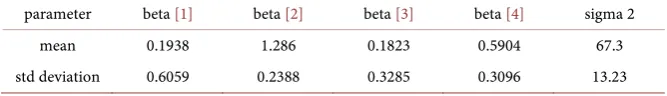
The hybrid algorithm described in Section 2.3 is used to generate simulations from the posterior distributions. After discarding the initial 500 draws for the burn-in, 10,000 draws are used for posterior inference. The posterior estimates (mean and standard deviation) of the model parameters are given in Table 1.
The Deviance Information Criteria (DIC) is commonly used for Bayesian model selection. The DIC is formed as the posterior mean of the deviance, which is -2 times the loglikelihood, along with a penalty for the effective number of pa-rameters ([12], Section 6.7). A second measure is the expected squared error loss (ESSE) given by
(
)
2, 1
T
t t obs
t
E y y
=
−
[image:9.595.206.540.677.725.2]
∑
, (15)Table 1. Posterior estimates of the CAPM for the SRA data.
DOI: 10.4236/jamp.2018.62031 330 Journal of Applied Mathematics and Physics where the expectation is respect to the posterior predictive distribution [22]. The quantity in Equation (15) corresponds to the posterior mean of the error sum of squares and does not include a penalty for model complexity. For the CAPM model fit result of this particular stock, the DIC is 366.6 and the ESSE is 3102.73.
[image:10.595.60.536.570.690.2]4.2. Evaluation of Fit of the CAPM
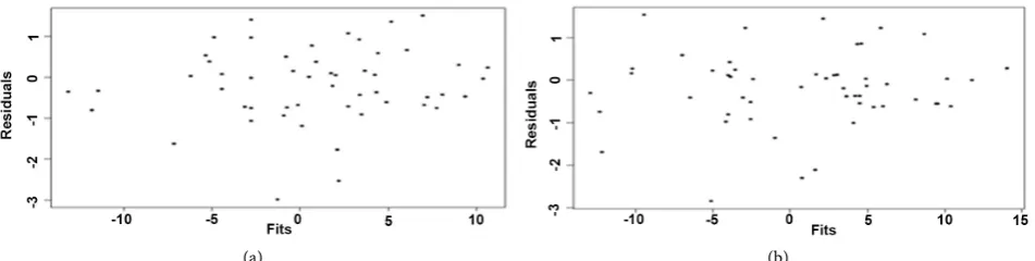
Figure 1 shows a plot of standardized Bayesian residuals in Equation (8) against the posterior mean values for each of the 52 monthly time points. This figure does not suggest any obvious departures from the homogeneity of variances as-sumption. However, it does show a few residuals with extreme negative values.
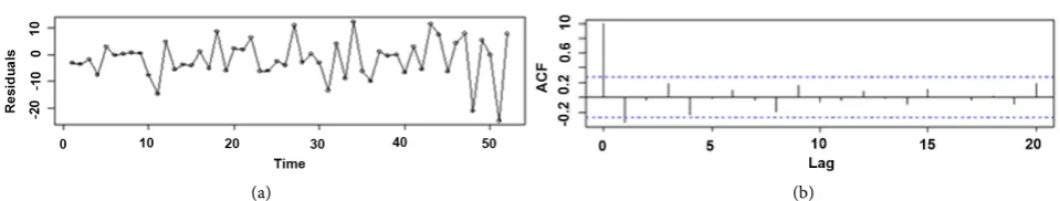
Figure 2 shows a plot of the residuals versus time as well as a plot of the auto-correlation function (ACF). In particular, the ACF plot in Figure 2 suggests the model errors may contain autocorrelation of order 1 since the ACF exceeds this threshold at lag 1. Figure 3 contains a histogram and normal quantile-quantile (QQ) plot of the standardized residuals. Both plots also highlight the extreme negative residual values. These small residual values are the only ones that tend to substantially deviate from the requisite line.
The three p-values in Section 3.2 can be used to quantify the degree to which model fit deviates from the required model assumptions. The classical p-value is computed by plugging in the posterior mean of the parameters as an estimate of θ in Equation (11). The ppp is calculated using Algorithm 3. The partial-ppp is calculated based upon Algorithm 4 as all test statistics are expected to be highly variable across the posterior draws.
A number of pivotal quantities could be used as measures of discrepancy
( )
,D eθ from the model assumptions. To quantify violations of independent errors, the Portmanteau test on the residuals is used. The associated Ljung-Box test statistic follows a Chi-squared distribution ([23], p. 541). To assess possible violation of the homogeneity of variance assumption, the Breusch-Pagan La grange multiplier test statistic is applied to the residuals. The test statistic is known to follow a Chi-squared distribution ([23], p. 510). To assess the assump-tion of normality, the Wilk-Shapiro test is applied to the residuals. With a
(a) (b)
DOI: 10.4236/jamp.2018.62031 331 Journal of Applied Mathematics and Physics (a) (b)
Figure 2. Time series plot and ACF plot of Bayesian residuals for the CAPM.
[image:11.595.65.541.188.273.2](a) (b) Figure 3. Histogram and normal Q-Q plot of Bayesian residuals for the CAPM.
normalizing transformation, the test statistic follows a standard normal distribu-tion [24].
The p-values presented in Table 2 confirm that there is no evidence against the homogeneity of variance assumption. There is some evidence against the normality assumption, though the ppp and partial-ppp show the evidence is not strong. The lack of normality is likely attributable to the two smallest residual values. The classical p-values and the partial-ppp show evidence against the as-sumption that the model errors are independent. The ppp appears to be a bit more conservative for this test. The Portmanteau test is used to detect that there is evidence that the model errors have lag 1 autocorrelation.
4.3. Fit of the CAPM with Autocorrelated Errors
The evaluation of the model fit in Section 4.2 revealed some evidence of a dis-crepancy from the assumption of independent model errors. The approach of
[25] can be used to incorporate autocorrelation into the CAPM. This approach will be used in this subsection to model first-order autocorrelation (AR(1)). Thus, the model in Equation (2) is now represented as
t t t
y =x′β+ε , with εt=φεt−1+at, and
(
)
2
~ 0,
t
a N σ . (16) It is convenient to reparameterize the model in Equation (16) using the Prais- Winsten transformation [26]. Under this reparameterization,
* *
t t t
y =x′β+a, with *
1
t t t
y =y −φy− , and xt*=xt−φxt−1. (17) The model errors at for this transformed model should satisfy the usual
as-sumptions listed in Equation (16) for t=2,,T. This model can be written in
the same form as Equation (3), but with *
y in place of y and X* in place of X .
DOI: 10.4236/jamp.2018.62031 332 Journal of Applied Mathematics and Physics Table 2. P-Values for the fit of the CAPM to the SRA data.
check classical ppp partial-ppp
Lag 1 Corr. 0.0364 0.0791 0.0460
Equal Var 0.8915 0.8216 0.8791
Normality 0.0623 0.1049 0.0953
( )
(
2)
1 2 ~ 1f φ −φ − . Thus, the parameter vector θ is now β σ φ ′2 . The posterior simulation is performed using the hybrid algorithm involving both the M-H procedure and Gibbs sampling as follows. The updating of
β
andφ
is conducted via the Gibbs sampler in Algorithm 2 using the full conditionals from[25]. The updating of σ2 is conducted via the M-H procedure described in Algorithm 1.
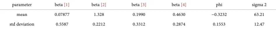
After discarding the initial 500 draws for burn-in, 10,000 draws are used to obtain the posterior estimates. These estimates are given in Table 3. The new model has a DIC of 364.6 and squared error loss of 3075.09. Based upon these goodness-of-fit measures alone, the Prais-Winstern reparameterization of the CAPM would be preferred. The next section provides diagnostic checks on this proposed model.
4.4. Evaluation of Fit of the CAPM with Autocorrelated Errors
The residuals in Equations (9) and (10) can also be used for the CAPM with au-tocorrelated errors given in Equation (16). These residuals are based upon *y and *
X defined in Section 4.3. Figure 1 shows the plot of the corresponding standardized Bayesian residuals against the posterior mean values for each of the 52 monthly time points based upon the CAPM with autocorrelated errors. This figure does not suggest any obvious departures from the homogeneity of va-riances assumption. However, there are again a few residuals with extreme nega-tive values. Figure 4 shows a plot of the residuals versus time as well as a plot of the autocorrelation function (ACF). The plot of the residuals against time in
Figure 4 looks similar to Figure 2. However, the ACF plot in Figure 4 no longer suggests the presence of autocorrelation of any order. Figure 5 contains a histo-gram and a normal quantile-quantile plot of the residuals. Both plots show the extreme negative residual values. The distribution of the model errors may have tails that are too heavy for the normal assumption to hold.
DOI: 10.4236/jamp.2018.62031 333 Journal of Applied Mathematics and Physics Table 3. Posterior estimates of the CAPM with autocorrelated normal errors for the SRA data.
parameter beta [1] beta [2] beta [3] beta [4] phi sigma 2
mean 0.07877 1.328 0.1990 0.4630 −0.3232 63.21
[image:13.595.59.540.175.347.2]std deviation 0.5587 0.2212 0.3312 0.2874 0.1553 12.47
Table 4. P-Values for the fit of the CAPM with autocorrelated normal errors to the SRA data.
check classical ppp partial-ppp
Lag 1 Corr. 0.6397 0.5080 0.4073
Equal Var 0.4337 0.4352 0.2108
Normality 0.0142 0.0750 0.0471
[image:13.595.70.534.386.467.2](a) (b) Figure 4. Time series plot and ACF plot of Bayesian residuals for the CAPM with corrrelated normal errors.
(a) (b)
Figure 5. Histogram and normal Q-Q plot of Bayesian residuals for the CAPM with corrrelated normal errors.
4.5. Fit of the CAPM with Autocorrelated
t
Errors
In order to address the problem of heavy tails in the fit of the CAPM with auto-regressive normal errors, one approach is to use the t-distribution to model the likelihood. A modification of Equation (17) to accommodate the t-distribution is given by
* *
t t t
y =x′β+a , with at~Tdf
(
0,σ2)
. (18) The proper degrees of freedom (df) for the t-distribution can be determined using an exploratory method assuming the non-informative prior density( )
1df ~ Uniform 0,1 . This form of prior is recommended over the more obvious choice of df ~ Uniform 1,
( )
∞ because the latter essentially has all its mass neardf = ∞ ([27], p. 193). For the SRA data, the posterior distribution of df
cen-ters around the value of 10 which is taken to be the value for the degrees of free-dom.
DOI: 10.4236/jamp.2018.62031 334 Journal of Applied Mathematics and Physics for each at can be represented as
(
)
| ~ 0,
t t t
a h N h and ht~ IG
(
df,σ2)
, (19) where the variables ht are auxiliary variables that cannot be directly observed.There is no direct way to compute ht, but it is straightforward to obtain the
conditional posterior distribution ([12], p 303) as
(
)
2
2
2 * *
1 2
| , , , ~ IG ,
2
t
t t
df h
df y
σ φ
σ
+
⋅ + −
y
x β
β . (20)
The posterior simulation can be performed using a hybrid algorithm involv-ing both the M-H procedure and Gibbs samplinvolv-ing. The updatinvolv-ing of
β
,φ
, htis done via the Gibbs sampler in Algorithm 2. The updating of σ2 is achieved via the M-H procedure described in Algorithm 1. All prior distributions remain the same for this model. The software program WinBUGS is used to obtain 10000 posterior draws after the 500 burn-in draws. Estimates under this model are given in Table 5. For the goodness-of-fit measures, DIC is 364.7 and the squared error loss is 3087.24. According to these criteria, the performance of this model is better than the CAPM in Section 4.1 and similar to the CAPM with au-tocorrelated normal errors in Section 4.3.
4.6. Evaluation of Fit of the CAPM with Autocorrelated
t
Errors
According to Equation (18), the model errors should have a t-distribution. Note that this corresponds to the marginal distribution of at across the values of htin Equation (19). Given values of ht, the conditional distribution of a ht| t is
normal. Thus, for each draw from the posterior distribution, observed residuals are calculated using Equation (9). Values of ht are also drawn according to
Equation (20). Then the observed residuals are standardized by dividing by ht
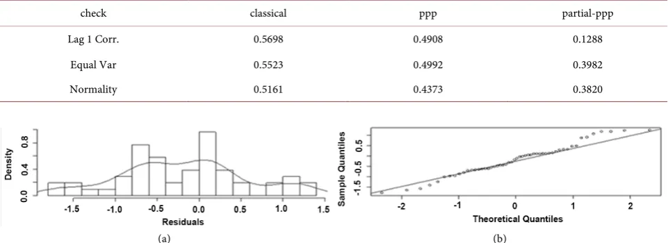
as opposed to a function of σ based upon the t-distribution in Equation (18). The histogram and normal quantile-quantile plot of these standardized residuals are shown in Figure 6. The normal quantile-quantile plot shows some of the same deviations from the requisite line in the tails as that observed in Figure 5. However, the scaling from the t-distribution has substantially reduced the mag-nitude of these deviations at the tails. As a result, these residuals are closer to the reference line required for the normality assumption.
The p-values are provided in Table 6. The p-values for the test of normality show no evidence against the normality assumption. The p-values also show no evidence against the homogeneity of variance assumption or the independence assumption.
5. Conclusions
DOI: 10.4236/jamp.2018.62031 335 Journal of Applied Mathematics and Physics Table 5. Posterior estimates of the CAPM with autocorrelated t errors for the SRA data.
parameter beta [1] beta [2] beta [3] beta [4] phi sigma 2
mean 0.1708 1.336 0.1875 0.5036 −0.2830 54.55
[image:15.595.58.539.178.353.2]std deviation 0.5320 0.2243 0.3507 0.2944 0.1577 11.68
Table 6. P-Values for the fit of the CAPM with autocorrelated t errors to the SRA data.
check classical ppp partial-ppp
Lag 1 Corr. 0.5698 0.4908 0.1288
Equal Var 0.5523 0.4992 0.3982
Normality 0.5161 0.4373 0.3820
(a) (b) Figure 6. Histogram and normal Q-Q plot of Bayesian residuals for the CAPM with corrrelated t errors.
include the use of (standardized) observed residuals and (standardized) realized residuals as discrepancy statistics. The Bayesian residuals can be plotted to vi-sualize possible violations of the model assumptions. Posterior probabilities can be used to quantify the amount of discrepancy. Specific assessments in this study included checks of autocorrelated errors, heterogeneous variances, and non- normality. Such Bayesian diagnostic approaches would be suitable for other li-near regression models and for general lili-near models that have correlated ob-servations.
[image:15.595.57.539.178.352.2]DOI: 10.4236/jamp.2018.62031 336 Journal of Applied Mathematics and Physics
Acknowledgements
This research was supported in part by a Basic Research Grant from the College of Arts and Sciences at the University of Wyoming, Laramie, WY USA. The au-thors would also like to thank an anonymous referee for their comments and suggestions.
References
[1] Fama, E.F. and French K.R. (1993) Common Risk Factors in the Returns on Stocks and Bonds. Journal of Financial Economics, 33, 3-56.
https://doi.org/10.1016/0304-405X(93)90023-5
[2] Pastor, L. and Stambaugh, R.F. (1999) Cost of Equity Capital and Model Mispricing.
Journalof Finance, 54, 67-121. https://doi.org/10.1111/0022-1082.00099
[3] Lo, A.W. (2000) Finance: A Selective Survey. Journal of American Statistical Asso-ciation, 95, 629-635. https://doi.org/10.1080/01621459.2000.10474239
[4] Tsay, R.S. (2002) Analysis of Financial Time Series. John Wiley & Sons, New York. https://doi.org/10.1002/0471264105
[5] Brav, A. (2000) Inference in Long-Horizon Event Studies: A Bayesian Approach with Application to Initial Public Offerings. The Journal of Finance, 55, 1979-2016. https://doi.org/10.1111/0022-1082.00279
[6] Campbell, J.Y., Lo, A.W., and MacKinlay, A.C. (1997) The Econometrics of Finan-cial Markets. Princeton University Press, New Jersey.
[7] Zellner, A. (1971) An Introduction Bayesian Inference in Econometrics. John Wiley & Sons, New York.
[8] Hastings, W.K. (1970) Monte Carlo Sampling Methods Using Markov Chains and Their Applications. Biometrika, 57, 97-109. https://doi.org/10.1093/biomet/57.1.97 [9] Gelfand, A.E. and Smith, A.F.M. (1990) Sampling-Based Approaches to Calculating
Marginal Densities. Journal of the American Statistical Association, 85, 398-409. https://doi.org/10.1080/01621459.1990.10476213
[10] Little, R. (2006) Calibrated Bayes: A Bayes/Frequentist Roadmap. American Statisti-cian, 60, 213-223. https://doi.org/10.1198/000313006X117837
[11] Pettit, L.I. (1986) Diagnostics in Bayesian Model Choice. The Statistician, 35, 183-
190.https://doi.org/10.2307/2987522
[12] Gelman, A., Carlin, J.B., Stern, H. and Rubin, D.B. (2003) Bayesian Data Analysis. 2nd Edition, Chapman and Hall, London.
[13] Gelman, A., Meng, X.L. and Stern, H. (1996) Posterior Predictive Assessment of Model Fitness via Realized Discrepancies. Statistica Sinica, 6, 733-807.
[14] Carlin, B.P. and Louis, T.A. (2000) Bayes and Empirical Bayes Methods for Data Analysis. 2nd Edition. Chapman and Hall/CRC, Boca Raton.
https://doi.org/10.1201/9781420057669
[15] Meng, X.L. (1994) Posterior Predictive P-values. The Annals of Statistics, 22, 1142- 1160.https://doi.org/10.1214/aos/1176325622
[16] Bayarri, M.J. and Berger, J.O. (2000) P Values for Composite Null Models. Journal of the American Statistical Association,95, 1127-1142.
https://doi.org/10.2307/2669749
DOI: 10.4236/jamp.2018.62031 337 Journal of Applied Mathematics and Physics 95, 1143-1156.
[18] Bayarri, M.J. and Berger, J.O. (1999) Quantifying Surprise in the Data and Model Verification. In: Bernardo, J.M., Berger, J.O., Dawid, A.P. and Smith, A.F.M., Eds.,
Bayesian Statistics 6, Oxford University Press, Oxford, 53-82.
[19] Bayarri, M.J., Castellanos, M.E. and Morales, J. (2006) MCMC Methods to Ap-proximate Conditional Predictive Distributions. Computational Statistics & Data Analysis, 51, 621-640.https://doi.org/10.1016/j.csda.2006.01.018
[20] Johnson, V.E. (2007) Bayesian Model Assessment using Pivotal Quantities. Bayesian Analysis, 2, 719-734.https://doi.org/10.1214/07-BA229
[21] Box, G.E.P. (1980) Sampling and Bayes’ Inference in Scientific Modeling and Ro-bustness. Journal of the Royal Statistical Society, Series A, 143, 383-430.
https://doi.org/10.2307/2982063
[22] Gelfand, A.E. and Ghosh, S.K. (1998) Model Choice: A Minimum Posterior Predic-tive Loss Approach. Biometrika, 85, 1-11.https://doi.org/10.1093/biomet/85.1.1 [23] Greene, H.W. (2000) Econometric Analysis. 4th Edition, Prentice Hall, Upper
Sad-dle River.
[24] Royston, J.P. (1982) An Extension of Shapiro and Wilk’s W Test for Normality to Large Samples. Applied Statistics, 31, 115-124.https://doi.org/10.2307/2347973 [25] Chib, S. (1993) Bayesian Regression with Autoregressive Errors—A Gibbs Sampling
Approach. Journal of Econometrics, 58, 275-294. https://doi.org/10.1016/0304-4076(93)90046-8
[26] Prais, S.J. and Winsten, C.B. (1954) Trend Estimators and Serial Correlation. Cowles Commission Discussion Paper, No. 383.