Probing with low frequency electric currents

Probing With

Low Frequency

Electric Currents

A thesis

submitted for the degree of

Doctor of Philosophy in Electrical Engineering

from the

University of Canterbury,

Christchurch~

New Zealand

A. D. SEA GAR, B.E.(Hons)

."

LIBRARY THESIS

( i) ABSTRACT

Four aspects of probing with low frequency electric currents are considered.

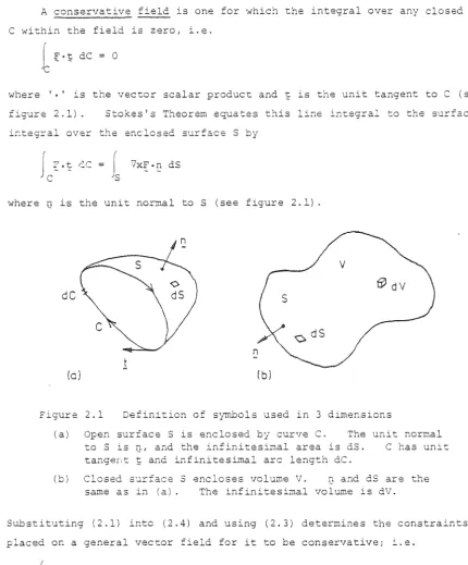
Applications of probing with electric currents in geophysics and medicine are reviewed. The theory of conservative fields is reviewed, and is discussed in relation to low frequency electric currents and other

physical phenomena to which i t applies.

The resolution with which a conductivity distribution can be recon-structed from electrical measurements is examined. Relationships are derived which relate the accuracy of the measurements to both the spatial resolution and conductivity resolution of the distribution. These relation-ships are obtained for conductivity distributions within both circular and half plane regions. It is found that the spatial resolution and conduct-ivity resolution at any point depend on both the location and the conduct-ivity of that point. It is experimentally verified that the best theor-etical value of spatial resolution, for measurements having a particular accuracy, can be closely approached in practice.

The relationship between two-dimensional circularly s~uetric conduct-ivity distributions and electrical probing measurements performed on them is studied. Two approaches are employed. One treats these distributions as smooth and the other treats them as piecewise constant. Two techniques are developed for reconstructing the conductivity distributions from the measurements. One technique is iterative whereas the other is direct. Examples are given in which these techniques are applied to a variety of simulated and experimental measurements. These examples show how we~.l conductivity distributions, reconstructed by these techniques, can be expected to represent the actual conductivity distributions.

The relationship between electrical probing measurements and general two-dimensional conductivity distributions is examined. These distributions are represented both as being smooth and piecewise continuous. Equations are developed relating the measurements on the boundary of a region to the conductivity distribution therein. The conditions on such measurements,

(ii)

different portions of the region can be neglected. These circumstances are experimentally verified. A direct technique is developed for inter-preting measurements in terms of a particular type of conductivity distrib ution. This technique is applied successfully to both experimental and simulated measurements.

ACKNOWLEDGEMENTS

I wish to express my sincere gratitude to my supervisor, Professor R. H. T. Bates, for all the support and encouragement he has provided throughout the course of this study. The benefit of his experience has contributed significantly to all stages of the work involved. I also wish to offer special thanks to Professor J. M. Gibbs and Dr. F. M. Davis of the Department of Anaesthesia of the Christchurch Clinical School of Medicine. Their guidance, insight and assistance was of great value to the medical aspects of this study.

Many thanks also to Dr. G. C. McKinnon, S. Fountain, L. S. Chan and M. J. Henderson for contributions to various aspects of the work reported in this thesis. I am also grateful to my colleagues at the Electrical Engineering Department who have provided companionship and shown interest in my research. In particular I wish to thank Don Mackay, Dr. Brent Robinson, Dr. Phil. Bones, Dr. Rick Millane, Richard Fright and Kathy Garden, with whom I have had helpful discussions.

(v) PREFACE

Information about a physical system is often obtained by interacting some form of energy with the system and measuring the resulting effects. Different forms of energy may be chosen according to the particular system being observed and the particular information desired about that system. The measurements themselves do not usually present the information in a manner which is readily understood, so that some form of processing is needed to uncover the wanted information. This thesis is concerned with obtaining information by interacting low frequency electric currents with physical systems. Two types of system are considered.

The first type of system is one which can be represented as a two-dimensional region in which the electrical conductivity is a function of position. This type of system is of particular relevance for geophysical prospecting and medicine. For the former, the conductivity distribution throughout a region of the earth is related to the minerals, rocks, liquids and gases of which the region is composed. Similarly, in medical applic-ations, the conductivity distribution throughout a region of the human body is related to the tissues and fluids of which the region is composed.

In both geophysics and medicine the objective of making electrical measure-ments is to obtain the conductivity distribution, and then from that to infer the material composition of the region. In geophysics this inform-ation may be used to locate regions of particular interest, such as certain geological structures or types of rock. In medicine the information is potentially useful as an aid to diagnosis of certain medical conditions.

Chapter 1 of this thesis contains a review of the different electrical probing techniques used in both geophysics and medicine. The literature indicates that in both of these areas there is at present an interest in imaging two-dimensional conductivity distributions from electrical measurements. Chapter 2 contains a review of the theory pertaining to conservative fields. It is this theory which describes

flow of low frequency electrical currents through conductive regions. Conservative field theory applies to a wider range of situations than just electrical measurements on conductive regions, as is explained in detail in Chapter 2. The original work presented in this thesis is described in Chapters 3 to 6.

The accuracy to which a conductivity distribution can be imaged is the main factor determining the practical usefulness of an image of the distribution. This accuracy is always limited by experimental errors in the measurements. In Chapter 3 the manner in which such errors limit both the spatial resolution and conductivity resolution of an image are examined. These limits are determined for conductivity distributions existing within regions whose shapes are either circles or half planes. The limits apply-ing to the former type of region are of particular relevance to medical probing, whereas those applying to the latter region are of particular

relevance to geophysical probing. The imaging accuracy may also be limited by incompleteness of measurements or assumptions about the geometry of the conductive region. These limits are also investigated in Chapter 3.

Two methods for imaging two-dimensional circularly symmetric

conductivity distributions are examined in Chapter 4 as a precursor to the study of general two-dimensional conductivity distributions. One of the methods is iterative and the other is direct. These methods are used to

image distributions from both simulated and experimental measurements. Using such measurements, case studies are performed in order to evaluate the effects which different factors have on the images. The effects of premature terminatior. of the iterative method and the effect of noise in the measurements are examined.

(vii)

regions. It is important to ensure that these conditions are fulfilled when making probing measurements, otherwise i t is not possible to uniquely determine the conductivity distribution being probed. A series of case studies are examined in order to draw useful conclusions about the relation-ship between the conductivity distribution and the measurements. In partic-ular, the effects of neglecting coupling between different regions within the distribution are examined. A direct technique is developed for imaging a particular type of conductivity distribution. This technique is applied to measurements obtained both from experiments and simulations.

In Chapters 3, 4 and 5 results based on both simulations and experi-ments are presented. The simulations were performed using the theory derived in the earlier sections of those chapters. The experiments were performed using a system developed for that purpose. This system is described in Appendices 1 and 2.

Venous occlusion plethysmography is a technique which is a useful aid in the diagnosis of peripheral venous disease. This technique involves interrupting the venous bloodflow out of a limb without affecting the arterial bloodflow into the limb. The limb increases in volume as blood collects in it. After 30 to 60 seconds the interruption is removed and the volume of the limb returns to normal. In Chapter 6 a model is developed for interpreting these changes in limb volume. The model is designed so that i t has parameters which are related as closely as possible to the physio-logy of the circulatory system within the limb. This approach allows the values of the model parameters, for which the model mimics a particular

change in limb volume, to be readily interpreted in terms of limb circulation. The model is also designed to be sufficiently simple for the values of the model parameters to be uniquely determined from such changes in volume. The model is shown to be related to alternative methods of interpreting the changes in limb volume, and i t is discussed in relation to these methods. The experimental measurements reported in this chapter were made using an impedance plethysmograph, which was designed and built as part of this study. The impedance plethysmograph is described in Appendix 2. The plethysmograph also forms part of the measurement system referred to above.

During the course of the work presented in this thesis the follow-ing papers and presentations were prepared.

R. H. T. Bates, G. C. McKinnon and A. D. Seagar. 1980.

"A Limitation on Systems for Imaging Electrical Conductivity". IEEE. Transactions on Biomedical Engineering, V27 #7 July pp418-420.

A. D. Seagar, J. M. Gibbs and R. H. T. Bates. 1980.

"Impedance Imaging and Plethysmography". Presented at the 20th Conference on Physical Sciences and Engineering in Medicine and Biology, Christchurch, New Zealand, August 1980. Abstract: Conference Proceedings p49.

K. L. Garden and A. D. Seagar. 1982.

"Low Frequency Electrical Current Measurements as an Aid to Medical Diagnosis". Presented at NZIE Annual Conference, Christchurch, New Zealand, February 1982. Abstract: Conference Papers p17.

R. H. T. Bates, J. H. T. Bates, P. J. Bones, R. P. Millane and A. D. Seagar. 1982.

"Computational Aspects of Physiological System Modelling". Presented at the Australian National Bio-Medical Engineering Conference, Melbourne, Australia, November 1982. Abstract: Book of Abstracts p4.

J. H. T. Bates, W. R. Fright, R. P. Millane, A. D. Seagar, A. E. McKinnon and R. H. T. Bates. 1982.

"Subtractive Image Restoration III: Some Practical Applications". Optik, V62 #4 pp333-346.

A. D. Seagar, J. M. Gibbs and F. M. Davis. 1982.

"Interpretation of Venous Occlusion Plethysmographic Measurements using a Simple Model". Submitted to Medical and Biologi..cal Engineering and Computing.

F. M. Davis, ,J. A. Floate, V. G. Laurenson, W. J. Gillespie and A. D. Seagar. 1982.

TABLE OF CONTENTS

ABSTRACT

ACKNOWLEDGEMENTS

PREFACE

CHAPTER 1 1.1

1.2

1.3

1.4

1.5

CF..APTER 2 2.1 2.2 2.3

PROBING WITH ELECTRIC CURRENTS Introduction

1.1.1 Probing Geophysical Probing 1. 2.1

1.2.2 1.2.3 1.2.4 1.2.5

Electrical Properties of the Earth Measurements on the Earth

Simplified Models

Interpretation of Measurements Uniqueness and Resolution Medical Probing

1.3.1 1. 3.2 1. 3.3

Electrical Properties of Tissue Impedance Plethysmography

Medical Uses of Plethysmography Impedance Imaging

Projection Images 1.4.1

1.4.2 1.4.3

Back Projection

Iterative Model Fitting Discussion

CONSERVATIVE FIELDS Introduction

Potential, Flux and Sources Electric and Magnetic Fields 2.3.1 _{Static Electric Field} 2.3.2 _{Static Magnetic Field} 2.3.3 _{Static Electric Field}

in

in

a Dielectric

a Conductor 2.3.4 _{Quasi-static Electric and Magnetic Fields} 2.3.5 _{Current Flow in a Quasi-static Electric Field}

(ix)

PAGE

(i)

( i i i )

I

(xl

2.4

2.5 2.6

Other Kinds of Fields 2.4.1

2.4.2 2.4.3

Fluid Flow

Diffusion and Heat Conduction Gravitation

Tabulated Summary

Integral Equation Representation 2.6.1

2.6.2 2.6.3

Greens Function for Poisson's Equation Equation for Continuously Varying Regions Equation for Piecewise Homogeneous Regions 2.7 Laplaces Equation

2.7.1 2.7.2

Separation of Variables Conformal Mapping

CHAPTER 3 LIMITATIONS ON IMPEDANCE IMAGING 3.1

3.2

Introduction

The Circularly Symmetric Conductivity Distribution 3.2.1

3.2.2

Visibility and Spatial Resolution

Sensitivity and Conductivity Resolution

3.3 Conformal Transformation to Other Conductivity Distributions 3.3.1

3.3.2 3.3.3

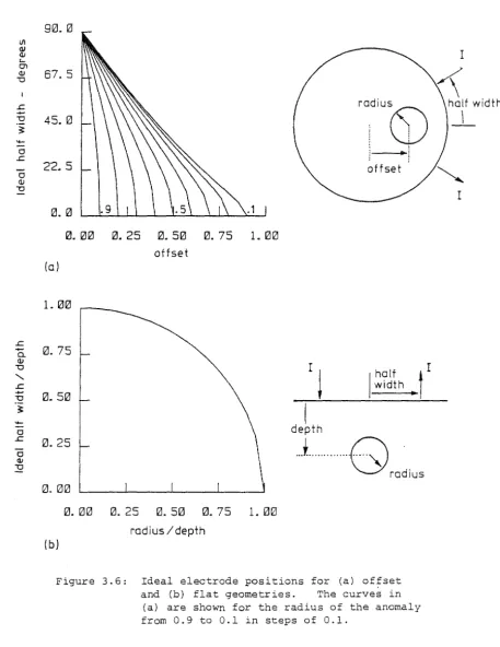
Ideal Electrode Positions

Maximum Visibility and Sensitivity Visibility Attained in Practice 3.4 Further Limitations of the Flat Geometry

3.5

CHAPTER 4 4.1

3.4.1 3.4.2

Incomplete Measurements

Approximation to a Curved Geometry Discussion

CIRCULARLY SY~.METRIC CONDUCTIVITY DISTRIBUTIONS Piecewise Constant Distributions

4.1.1

4.1. 2

Comparison Between Experimental and Simulated Measurements

Multiple Ring Models for Iterative Modelling 4.2 Smooth Conductivity Distributions

4.2.1

4.2.2

Comparison of Smooth and Piecewise Constant Distributions

Imaging Smooth Distributions

4.3

4.4

CHAPTER 5 5.1

5.2

5.3

5.4 5.5

Case Studies 4.3.1

4.3.2 4.3.3 4.3.4 4.3.5

Model Sensitivity to Data Fit

Effect of Random Noise in Measurements Alternative Choice of Models

Measurement Noise in Practice

Experimental Measurements Interpreted Using Three Models

Discussion

GENERAL CONDUCTIVITY DISTRIBUTIONS Smooth Distributions

5.1.1 5.1. 2 5.1. 3 5.1.4 5.1.5 5.1.6 5.1. 7 5.1.8

Description of Approach

Manipulating Poisson's Equation

Matching the Voltage Boundary Conditions Matching the Current Density Boundary Conditions

Relation Between Boundary Voltage and Current Density

Calculating the Transfer Impedances from Measurements

Receprocity in Relation to the Transfer Impedances

Simple Current Distributions for Making Measurements

Piecewise Constant Distributions 5.2.1

5.2.2

5.2.3

5.2.4 5.2.5

The Multiple Offset Anomaly Distribution Relation Between Boundary Voltage and Current Density

Three Components Contributing to Boundary Voltage

The Single Offset Anomaly Distribution

Direct Inversion for a Single Offset Anomaly Case Studies

5.3.1 5.3.2 5.3.3 5.3.4

Voltage Measurements and Transfer Impedances Transfer Impedances and Visibilities

Coupling Effects Between Two Anomalies Multiple Offset Anomalies and Coupling Single Offset Anomaly Reconstructions

CHAPTER 6

6.1 6.2

6.3

6.4

CHAPTER 7 7.1 7.2 7.3 7.4 7.5

MODELLING LIMB VOLUME CHANGES MEASURED DURING VENOUS OCCLUSION PLETHYSMOGRAPHY

Venous Thrombosis and Pulmonary Embolism The Model of the Limb Circulation

6.2.1 Using the Model to Represent Measurements Experimental Studies

6.3.1

6.3.2

6.3.3

Comparison of Model of Limb Circulation with Human Limbs

Relating the Model Parameters to Physiological Quantities

Modelling Limb Bloodflow, Compliance and Resistance Discussion

CONCLUSIONS AND SUGGESTIONS FOR FUTURE RESEARCH Limitations on Impedance Imaging

Circularly Symmetric Conductivity Distributions General Conductivity Distributions

Conservative Field Imaging

Modelling Limb Volume Changes Measured During Venous Occlusion Plethysmography

PA 15 15 15 16 16 16 16 16' 16'

17 ~ 17' 171 171 17(

17(

APPENDIX l ' SYSTEM FOR ELECTRICALLY PROBING CONDUCTIVITY DISTRIBUTIONS 18:

APPENDIX 2 INSTRUMENTATION

A2.1 Impedance Plethysmograph A2.1.1 Specifications A2.1.2 Circuitry A2.2 Analogue Multiplexer

APPENDIX 3 TECHNIQUES EMPLOYED FOR MODEL FITTING A3.1 Newton Methods

A3.2 The M0cre Penrose Generalised Inverse A3.3 Orthogonal Decomposition

A3.4 The Procedures Employed

APPENDIX 4 A POWER SERIES REPRESENTATION FOR THE QUOTIENT OF TWO POWER SERIES

APPENDIX 5

APPENDIX 6

REFERENCES

DETAIL OF SECTION 5.1.2

A DIRECT METHOD FOR ESTIMATING A SINGLE EXPONENTIAL CURVE FROM MEASUREMENTS

(xiii)

PAGE

203

209

1. PROBING WITH ELECTRIC CURRENTS

1.1 INTRODUCTION

Probing and sensing techniques are used in many areas of scientific and technical importance to gain useful or interesting information. This thesis is concerned with using low frequency electric currents to determine useful information from the spatial or temporal variation of conductivity.

(Low frequency means low enough for a conservative field approach to be applicable. See §2.3.4). Two areas in which electrical probing finds major application are geophysical prospecting and medical diagnosis.

Usually, the conductivity is only a convenient intermediary from which some other property is inferred. Where this is the case electrical probing may be only one of a variety of possible techniques. In geophys-ical prospecting the subsurface composition of the earth is sought, and an alternative method to probing with electric currents is to drill a hole and collect rock samples for analysis. One difference between the electrical method and such an alternative is that the former is non-invasive. This is not necessarily an advantage in geophysical prospecting, but i t is very much an advantage in medical diagnosis, where patient welfare is of paramount importance. This chapter serves as an introduction to, and a review of, electrical probing techniques used in geophysical prospecting and in medical diagnosis.

1.1.1 Probing

The generalised probing (or scattering) problem (cf. Bates and McKinnon 1980) is conveniently described with reference to figure 1.1. An incident emanation

W.

1 which is generated by a source (transmitter)

l

impinges upon and interacts with a region R of unknown physical properties

A,

giving rise to a perturbed ("scattered" is often an appropriate term) emanation ~ _s . The total emanation ~

=

~. + ~ is measured with a receiver

l s

(detector) and contains all

0=

the observable information about

A.

Forward probing involves finding ~ when ~. and

A

are known.

l Inverse

proting involves finding

A

when ~. and ~ are known. When the source is l

2

SOURCE RECEIVER

0

--

₀

lfJj

[image:15.600.135.495.130.522.2]

""

/

lfls

Figure 1.1: Generalised Probing (Scattering) Problem. Incident emanation ~. interacts with region R, which has physical characteristics

A,

and gives rise to scattered wavefunction ~s.

Inverse probing is mathematically more difficult to solve than forward probing. This is because the mathematical descriptions of physical phenomena are usually based on forward probing, and in many

situations i t is not clear how to manipulate such descriptions to solve inverse problems.

1.2 GEOPHYSICAL PROBING

1.2.1 Electrical Properties of the Earth

Electromagnetic fields can be useful for probing in geophysics

because different earth materials exhibit significant differences in conduct-ivity (or resistconduct-ivity p), permittconduct-ivity and permeability. The various

minerals found in the earth allow metallic conduction (e.g. native metals,

p

=

10-7 to 104

~m),

semicoDductor conduction (e.g. sulphides, p

=

10-4 to

a a

The electrical properties of the earth are seldom isotropic. Rock which is composed of a sequence of layers of isotropic constituents is effectively anisotropic because the current passes through a parallel com-bination of the constituents when flowing parallel to the layers, but passes through a series combination when flowing perpendicular to the layers. The ratio of perpendicular to parallel resistivity ranges from 1 to 25 (Keller 1971 §4.1). Even when rock is not composed of layers i t may be anisotropic because of some preferred orientation of texture.

1.2.2 Measurements on the Earth

The electrical techniques used to determine the electrical properties of the earth may be classed according to (i) the types of incident and

perturbed emanations used to perform the probing, (ii) the information contained in the measurements, and (iii) the particular source-receiver geometry used to obtain the measurements. There are many alternatives in each of these classifications, with any particular measurement technique comprising one alternative from each of (i), (ii) and (iii) above. There-fore there are many different measurement techniques.

Alternative Choices of Emanation

The types of emanation used to perform geophysical probing fall into 3 groups. There are conservative emanations (i.e. low frequency conduction currents), natural source non-conservative emanations (i.e. telluric electro-magnetic fields), and man made non-conservative emanations (i.e. man made electromagnetic fields).

Direct current and induced polarisation (also called overvoltage) techniques employ low frequency electric currents passed through the earth using suitable electrodes. Frequencies below 100 Hz are used because this enables a conservative field approach to be adopted (see §2.3.4). Direct current techniques use either a direct current source which is periodically reversed in polarity, or a low frequency sinusoidal waveform (Keller and

Frischknecht 1966 §16). Their purpose is to measure the spatial distribution of the electrical characteristics of the material beneath the earth's surface. Induced polarisation techniques make use of either the transient behaviour in the time domain (cf. Seigel 1959) or the steady state behaviour in the

4

and conduction current. Alternative parameters called the "metal factor" and the "frequency effect" a:!:"e also used.

Magnetotelluric and telluric methods make use of the currents induced in the earth by the natural variations in the earth's magnetic field. At frequencies above 1 Hz the variations are primarily caused by lightning strokes, and below 1 Hz are thought to be caused by the interaction between radiation or particulate matter from the sun and the earth's atmosphere and magnetosphere (Keller and Frischknecht 1966 §28). In turn, the currents

induced in the earth give rise to time varying electric and magnetic fields. Using the magnetotelluric method the variations in the magnetic field and electric field are measured at one site. In contrast, when using the tell-uric method the electric field alone is measured at a number of sites. The former method allows the conductivity at a given site to be determined (cf. Larsen 1981; Oldenburg 1979), while the latter allows the conductivity at various sites to be compared. When the conductivity at one site is known by some independent means i t can be used as a reference, in which case the tell-uric method also permits the conductivity to be measured (Yungul 1966).

Electromagnetic methods are those in which artificially gene:!:"ated time varying electromagnetic fields are used to probe the earth. These methods are further subdivided according to whether the receiver is in the near field or far field of the source. Induction methods are those in which the fields are transmitted and received by ?oils, and the wavelength of the fields in air exceeds the source-receiver spacing. Frequencies between 100 Hz and 5 kHz are used (cf. Keller and Frischknecht 1966 §34). Radio wave methods use electric dipoles for source and receiver, with wavelengths in air being less than the source-receiver spacing (cf. Keller and Frischknecht 1966 Ch.7). Both conductivity and permittivity can be estimated by electromagnetic methods

(the permeability is usually 1) since the frequencies used are hi.gh enough for displacement current flow in ·the earth to be significant in comparison with conductive current flow, This is in contrast to the telluric and magneto-telluric methods, where only the conduction current in the earth is significan

There are many different electromagnetic techniques which measure diffe ent characteristics of the electric and magnetic fields. The wave t i l t metho uses the vertical and horizontal electric fields at one site (cf. Lytle et al 1976), whereas the ground wave attenuation method uses the amplitude of a trav elling electric field measured at different sites (cf. Maley 1971 §2.4).

spatial Information Content

Measurements of the total emanation ~, are made in order to determine the spatial distribution of the earth's electrical characteristics. Often the spatial distribution is assumed to vary only in one dimension. Measure-ment techniques which are used to derive information which depends solely on the electrical characteristics as a function of depth, are called sounding techniques. Similarly, profiling techniques are those used for estimating lateral variations of the electrical characteristics. Those measurement techniques used to derive information about the electrical characteristics varying in at least two dimensions are called imaging techniques.

Source-Receiver Geometry

The conductivity distribution and the geometrical relationship between the transducers (i.e. electrodes or antennas) used for injecting signals into the earth and for sensing their effects are both intimately related to the effects measured. The injecting transducers are called sources, and the sensing transducers are called receivers. Several source-receiver configur-at ions have become standard, and they are referred to as arrays. Figure 1.2 shows the Wenner, Schlumberger, Eltran and dipole-dipole arrays, which are examples of arrays used for the direct current and induced polarisation techniques. The dipole-dipole array also applies to the electromagnetic methods which employ electric and/or magnetic dipoles.

Apparent Resistivity

The apparent resistivity P

a is a quantity often inferred from measure-ments made using the various electrical probing techniques (cf. Keller and Frischknecht 1966 §17). The values actually obtained for the apparent resistivity depend upon both the resistivity of the earth and the particular technique employed. It is defined as the resistivity of a uniform region which would give rise to the same measurements as those obtained over the actual region being probed. The relationship between the apparent resist-ivity and the measurements is defined differently for each measurement technique. For the direct current technique i t is written as

KV/I, (1.1)

6

(0)

(b)

~~

~a-- 0 " 0 -(e)

\\\\\\ \ \ \ \ \ \ \ \ \ \ \ \ \ \ \ \ \ \ \ \ \ \ \

\\\\\\\\\'\\\\\\\\\® ~,,\\\\\\\\\\\\\\\\\\\\\\

1-0---1

o)b

;rr~

--e--

.-.b--(d)

o»e

F~gure 1.2: Arrays for Direct Current and Induced Polarisation geophysical probing. 'I' is a current source and

'V' is a voltage detector. The distance 'a' is called the array spacing.

(a) Wenner array

(b) Schlumberger array (c) Eltran array

(d) Dipole-Dipole array.

The apparent resistivity calculated from measurements over a uniform region is equal to the actual resistivity of that region. When the region is not uniform, the apparent resistivity is a convenient way of character-ising the measurements. However i t is worth emphasising that the apparent resistivities obtained using different measurement techniqyes over the same nonuniform region are not necessarily the same.

Depending on whether measurements are being made for sounding, profil-ing or imagprofil-ing, the apparent resistivity is measured with respect to one or more independent variables. Suitable variables are the frequency of the

is defined in figure 1.2) and the lateral position of the array on the earth's surface.

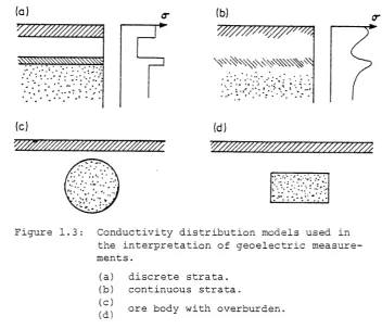
1.2.3 Simplified Models

In order to calculate the apparent resistivity of a region of the earth having a particular conductivity distribution, i t is necessary in general to be able to solveMaxwell'sEquations (see §2.3) in a nonhomogeneous anisotropic medium. As a mathematical simplification i t is often assumed that the earth conducts electricity isotropically. To further simplify the mathematics the conductivity distribution is often modelled in a simple

manner. Models with particular geological significance are the horizontally stratified earth and the isolated orebody with an overburden (see figure 1.3).

Many methods are available for calculating the apparent resistivity from conductivity distributions. These are divided here into 4 categories of modelling: (i) explicit, (ii) approximate, (iii) integral equation, and

(iv) scale.

(a)

(e)

~

.-.

,':'»-;::::",' .'

".:". _'. :

_.

.. ~'.,' .. :

~

.

'~

.

...

:.

~ .. , "

...

~'.~ ." ': " .

.... ~-.: ~

..

(b)

(d)

Figure 1.3: Conductivity distribution models used in the interpretation of geoelectric measure-ments.

(a) (b) (c) (d)

discrete strata. continuous strata.

[image:20.595.104.457.431.734.2]

8

Explicit Hodels

Explicit solutions of Haxwell's Equations are limited to relatively simple models. Nevertheless many useful solutions are known. The for-ward solution for direct current techniques over horizontally stratified media was originally developed for discrete strata (Stefanesco et al 1930; Keller and Frischknecht 1966 §23a) and has since been extended to allow for transition layers having a linear change in resistivity with depth (Hallick and Roy 1968; Koefoed 1979). Forward solutions for plane electromagnetic waves incident on stratified media have been developed for the calculation of magnetotelluric and telluric model data (Cagniard 1953; Wait 1981b Ch. 2,3) . The electromagnetic responses to various magnetic and electric sources over stratified media (Wait 1962 Ch.2; Dey and Ward 1970), over orebody models (Ogunade 1981) and over laterally inhomogeneous earth models

(Hill and Wait 1981) have been calculated to help with the interpretation of data gathered using electromagnetic methods.

Approximate Hodels

Smooth conductivity distributions are often approximated by piecewise constant distributions, as in finite element modelling (Coggon 1971; Kisner and Della Torre 1974; Pridmore 1981). The alternative finite difference modelling technique approximates the differential equation for the voltage

(see §2.3) by a difference equation (Hufti 1976, 1978; Dey and Harrison 1979). Transmission line (or network) modelling represents a multi-dimensional contin° uous conductivity distribution as a multi-dimensional mesh (or network) of one· dimensional resistors (Johns and Rowbotham 1981, Dines and Lytle 1981). The so-called alpha centre approach (which applies only to conservative fields) models the square root of the conductivity as a sum of continuous functions

(Stefanescu 1974; Petrick et al 1981). Solutions to the forward problem are facilitated by choosing these functions from appropriate sets.

Integral Equation Hodels

integ-Scale Models

Electromagnetic scale modelling involves building a model of the conductivity distribution and performing measurements on the model (cf. Frischknecht 1971). The model may be as complicated as desired. Scale modelling is particularly useful for providing experimental data to compare with calculated values obtained from any of the other three modelling methods discussed above.

1.2.4 Interpretation of Measurements

Curve Matching

The earliest method developed for the interpretation of sounding

measurements is called curve matching (cf. Keller and Frischknecht 1966 §20). The apparent resistivity is plotted as a function of the array spacing

(defined in figure 1.2), and the graph is compared to apparent resistivity curves for various stratified earth models (see figure 1.3a). The earth model with the apparent resistivity most closely matching that measured is taken to represent the region of the earth which is being sounded. In practice the curve matching technique is only capable of predicting two or three strata, since the number of possible models increases rapidly as the number of strata is increased.

Iterative Model Fitting

Any of the methods suitable for calculating the forward problem may be used as the basis of an iterative inverse method. Interpretation is performed indirectly by solving for the apparent resistivity for many para-meter values of a particular model. The set of parameters for which the apparent resistivity best fits the measurements is taken to be the solution. Any of the techniques available for function minimisation (cf. Gill and Murray 1974) are suitable for finding such a solution by minimising the difference (perhaps in a least squares sense) between the measured and cal-culated values for the apparent resistivity.

technique is largely arbitrary.

The choice of minimisation

Often there is insufficient independence in the data (perhaps due to noise) to arrive at a unique model. Regularisation techniques help to overcome this by selecting a solution subject to predetermined constraints

10

Stable iterative techniques have been developed for interpreting measurements in terms of stratified (i.e. one-dimensional) earth models. The models represent either continuous strata (Oldenburg 1978, 1979) or discrete strata (Parker 1971; Wu 1968; Glenn et al 1973; Rijo et al 1977; Meinardus 1970; Petrick et al 1977; Inman 1975; Vozoff 1958; Inman et al 1973) . These models are able to represent any earth stratification.

Iterative techniques which interpret measurements in terms of two and three-dimensional models have also been developed (Brass et al 1981; Pelton et al 1978; Petrick et al 1981), but they can only be applied to very simple kinds of conductivity distributions.

Ray Approximations

When the wavelength of an electromagnetic signal is small compared to any inhomogeneities in the refractive index, the propagation can be usefully approximated in terms of rays. Using this approach the reconstruction of two-dimensional cross sections is achieved in X-ray computed tomography (cf. Lewitt and Bates 1978a,b,c; Lewitt et al 1978; Kak 1979), ultrasound trans-mission tomography (Greenleaf et al 1974, 1975; Kak 1979), and in geophysical probing (Lytle and Dines 1980, Dines and Lytle 1979). In the latter situ-ation i t is more difficult to obtain the necessary data, since access to the entire circumference of the region being probed is not possible. Where ray curvature is important, due to changes in refractive index, correction schemes can be devised, although i t is far from clear at present whether they can be expected to be generally useful (cf. McKinnon and Bates 1980).

Direct Interpretation

Langer (1933) derives an analytical solution for the conductivity of a continuously stratified earth by relating a series representation of the con-ductivity to a function derived from the measurements. Slichter (1933) uses Langer's solution to compare the interpretation of some examples of conduct-ivity distributions. Langer's solution has been extended to allow for discon-tinuities in either the conductivity or its derivative (Langer 1936).

Pekeris (1940) develops a direct graphical technique to determine the conductivity of a discretely stratified earth. This technique is based on the asymptotic behaviour of the measurements at high spatial frequency (small array spacing). Beginning at the earth's surface and progressing downward each stratum is determined sequentially. This method has been automated

(Koefoed 1976) and modified to make i t more able to cope with noisy data

A third method, fundamentally different from the two described above, is that devised by Coen et al (1981) and Weidelt (1972). Nonlinear trans-formations are used to change the problem into an inverse scattering problem for the Schrodinger Equation. This can then be solved by the method of Gelfand and Levitan (1955).

1.2.5 Uniqueness and Resolution

The accuracy to which a conductivity distribution can be estimated, from data measured to a given accuracy, is not well understood. Often many significantly different conductivity distributions can be found, all of which are consistent with the measured data according to the accuracy of the measure-ments. This has been referred to as "non-uniqueness" or "equivalence".

Several methods are available for estimating the accuracy of the solution. Inman (1975) estimates the standard deviations of the model para-meters from the effect on the data of perturbations in the model. Altern-atively, Backus and Gilbert (1968) consider all solutions which when convolved with a point spread function are still consistent with the data.

mum width of the point spread function indicates the resolution.

The maxi-Roy and Apparao (1971) compare for different electrode arrays the contribution to the measurements given by a thin horizontal stratum (layer). This provides a measure of the relative ability of the various arrays to detec~ horizontal strata as a function of both depth and array spacing, thereby indicating the vertical resolution. Apparao and Gangadhara Rao (1974) use the same tech-nique for linear (as opposed to point) electrodes.

The accuracy to which a conductivity distribution is estimated can be improved when two different measurement techniques are used. This is achieved by interpreting both sets of measurements jointly, rather than each set

separately (Vozoff and Jupp 1975) .

1.3 MEDICAL PROBING

1.3.1 Electrical Properties of Tissue

I

1

12

lowest resistivity, e.g. 64 to 65 ~m for cerebrospinal fluid, and 61 to 67 ~cm for blood plasma (blood without the red blood cells). Amongst the poorest conductors are lung (140 to 2400 ~cm) f fat (1000 to 5000 ~cm) and bone (2000 to 16000 ~cm).

Materials of particular interest are skeletal muscle and blood. The resistivity of blood depends on the hematocrit (percentage of red blood cells) and on the velocity of the blood flow. It also depends on whether measurement is perpendicular or parallel to the direction of flow (Frewer 1974) f apparently being related to the spatial distribution and orientation of the red blood cells in the blood vessel. Typically the resistivity of blood is from 150 to 170 ~m. In contrast the resist-ivity of skeletal muscle is from 1 to 15 times higher than that of blood. Skeletal muscle is composed of many long parallel cells. Measured para-llel >lith the long axis of the cells the resistivity is from 150 to 408 ~cm, while in the perpendicular direction i t is from 675 to 2300 ~cm.

The cells of nerve and muscle tissue have membranes which are said to be electrically excitable (Katz 1966) . In the resting state an excit-able cell maintains an ionic concentration gradient across the cell mem-brane. This results in a resting potential difference, so that the membrane is said to be polarised. When the membrane is electrically stimulated its ionic permeability changes and allows the ionic concentrat-ions to equilibrate across the membrane. The resting potential disappears and the membrane is said to have depolarised. After a refractory period, during which the merrillrane is not excitable, or at least relatively insen-sitive to excitation, the cell membrane restores the ionic concentration difference and the resting potential returns. The variation with respect to time of the transmembrane potential, during the depolarisation and repolarisation of the membrane, is called the action potential.

found to be useful are the electromyogram (from skeletal muscle), the electroretinogram (being the response of the retina to visual stimulus), the electrooculogram (which is the variation in corneal-retinal potential accompanying eye motion), and the electrogastrogram (from the peristaltic movements of the gastrointestinal tract). These biologically produced potentials range from 10 ~V to 4 mV and from direct current to 100 Hz; or for the electromyogram up to 3 kHz (Cromwell et al 1973 Ch.3).

It is important that artificial electric potentials generated within the body for determining tissue conductivity do not interfere with the normal function of the body. Interference can cause effects such as ventricular fibrillation, where the muscle cells forming the ventricular chambers of the heart depolarise asynchronously so that the heart does not pump sufficient blood to maintain bodily function. Experiments on humans and other animals indicate that the threshold current required to elicit observable effects (such as the threshold of sensation, slowing of the heart due to interference with the vagus nerve, and ventricullar fibrillation) increases with the frequency of the applied current (Geddes et al 1969).

Electrical currents which do interfere with bodily functions can also induce beneficial effects. A large current pulse through the heart depolarises all ventricular tissue simultaneously allowing a heart undergoing ventricular fibrillation to return to normal synchronous operation.

Electrodes placed near nerves can be used to block the propagation of action potentials and induce an anaesthesia-like state (Geddes 1965).

The conductive properties of tissue can be measured in a variety of ways. Magnetic induction (cf. Tarjan and McFee 1968; McDonald 1979 Ch. 9), the attenuation of radio waves (Maini et al 1980) and the voltage resulting from current flowing through the tissue can all be used to find the conduct-ivity. The latter method requires electrodes to be connected to the tissue, and is widely applied in plethysmography (see §§1.3.2 and 1.3.3).

When using electrodes the useful frequency range of currents is limited, apart from the need for patient safety, by chemical effects at the electrode-electrolyte (tissue) boundary. A transfer of ions from the electrode into solution creates a static voltage, which in equilibrium balances the tendency of further ions to enter solution. This ionic

elect-14

rode connected via its saturated ionic solution to an abraded patch of tissue, to reduce the resistive component of impedance. When measuring high frequency voltages the capacitive component is negligible (Nowotny and Nowotny 1980) and elec~rode preparation is not so important.

1.3.2 Impedance Plethysmography

Plethysmography is the name given to any technique used for measur-ing those volume changes of the human body which are associated with some physiological event. Plethysmography is used on either a particular body segment (e.g. limb, digit, torso) or on the whole body. There are many alternative plethysmographic techniques. The changes in volume can be measured by enclosing the body segment in a rigid box and measuring changes in volume or pressure of the fluid within the box, or flow of the fluid from the box (Sumner 1978). Alternatively a strain gauge can be used around the circumference of the body segment, or the electrical resistance of the body segment can be monitored (see figure 1.4a). The latter method is called impedance plethysmography (Nyober 1970), and is convenient to apply in practice.

The relationship between the electrical resistance measured during impedance plethysmography and the volume changes of a body segment, is

derived from the assumption that the body segment is composed of cylindrical sections that have constant resistivity (figure 1.4b).

resistance R of each section is 2

R

=

p,Q,

IV

The longitudinal

(1.2) where P is the resistivity, 2 is the length and V is the volume of the sectio Assuming that the electrodes cover the end surfaces, the total longitudinal resistance is

(1. 3)

where the subscripts t and b stand for tissue and blood respectively.

When some physiological change causes a small change in blood volume ~V, without changing the length of the section, the change in resistance ~R is

(1.<1,)

Assuming that the total volume V (= Vt+V

b) is approximately equal to VDPt/Pb+ (which is true when P

I

(e)

Figure 1.4:

A

1

L I

j

-~---~,

/ :

.

"-I

y---3

I ' _ _ J

(b)

(a) Impedance plethysmography performed on limb by passing current between one pair of circumferencial electrodes and monitoring voltage on another pair.

(b) Assumed electrical model of limb with end electrodes causing parallel current flow along cylindrical sections of constant resistivity.

(1.5)

L

j

Whereas the geometry of limbs, fingers and toes is reasonably approx-imated by cylinders, the torso of the body has many isolated inhomogeneities

(e.g. heart, lungs) and is not well approximated by a cylinder. Furthermore, electrodes are usually applied to the body segment as circumferential bands

I

16

When the section expands longitudinally instead of radially, its longitudinal resistance increases (Brown et al 1975). Depending on the ratio of longitudinal to radial stretching, the magnitude of the measured change in resistance is somewhat smaller than that given by (1.5). On average the measured value of ~R/R is 20% lower than if no longitudinal stretching were present (Jaffrin and Vanhoutte 1979), but the effect can be reduced by mounting the electrodes on an inextensible frame. The change in conductivity of blood with blood velocity contributes to the measured change in resistance (Swanson and Webster 1976), and can contrib-ute as much as 10% of ~R/R as do volume changes (Peura et al 1978).

1.3.3 Medical Uses of Plethysmography

Venous Occlusion Plethysmography

Venous occlusion plethysmography is the measurement of volume changes of a body segment during an interval when the venous bloodflow is first occluded and then subsequently restored. A convenient way to achieve venous occlusion is to inflate a pneumatic cuff encircling the limb to a pressure in excess of venous pressure but lower than arterial pressure (see figure 1. Sa) . The body segment increases in volume as blood collects in the veins. On release of the pressure within the cuff, the limb volume returns to its previous level (see figure 1.Sb).

t

__ - - I I

t

t

+

(a) cuff inflated

,

(b) cuff deflated

t

time

Figure 1.5: Volume changes measured during venous occlusion plethysmography.

The volume change is about 1% of the volume of the body segment, and contains two diagnostically important pieces of information. The slope of the curve immediately after occlusion is proportional to the bloodflow into the limb (cf. Sumner 1978). The shape of the volume decay following the release of occlusion is useful in the diagnosis of venous thrombosis, which is the blockage of veins due to blood clots.

Several methods have been developed in order to diagnose venous thrombosis from the limb volume change measured during venous occlusion plethysl!lography (cf. Barnes et al 1972; Johnson & Kakkar 1974; Nheeler

et al 1974). These methods involve deducing one or two parameters from the volume change (see figure 1.6), and using the parameters as an aid to diagnosis.

volume change

(a)

(c)

(b)

Figure 1.6: Alternative parameters used to interpret venous occlusion volume changes for venous throrr~osis.

(a) the rate of decrease in volume at cuff release (Barnes et al 1972) ,

(b) the ratio of the fall in volume in the 2 seconds following cuff release to the total rise in volume (Johnson & Kakkar 1974) I

(c) the fall in volume in the 3 seconds following cuff release together with the rise in volume

(Wheeler et al 1974),

(d) the half life of the decrease in volume following cuff release (Jaffrin 1976) .

Pulse Plethysmography

Pulsatile volume changes of body segments are observed every time the heart beats. The volume change is due to periodic fluctuations in the

18

(excluding the torso) (see figure 1. 7) . The pressure pulse originates at the heart and travels towards the peripheral parts of the body. As the pulse travels down the arterial tree, its shape and amplitude change accord-ing to the physiological state of the vessels through which i t passes. The shape of the volume change at the extremities is useful in the diagnosis of arterial occlusive conditions (arteriosclerosis) (cf. Raines 1978).

0.08

(aJ

~ 0

(1) 0

01 C

0

L.

Cl .J::.

U Q)

0.08

E

::l "'6 >

{bJ

o

o

L.

time - seconds

Figure 1.7: Pulsatile volume changes measured simultaneously on the

(a) upper arm, and (b) lower leg (calf).

Quantitative interpretaion of the pulsatile volume change is complic-ated by two factors. Firstly, non-pulsatile bloodflow has no effect on the measured volume change, so that absolute bloodflow cannot be determined

(Brown et al 1975). Secondly, differences between the pressure pulse at the heart amongst different individuals necessitates the use of some form of normalisation of peripheral pulse shape against pulse shape at the heart.

logical state of the vessels (Skidmore and Woodcock 1980; Brown et al 1978; Li et al 1980).

Cardiac Output

Pulsatile volume and impedance changes of the torso occur as the heart beats. It is clear that the changes are in some way related to the function of the heart and vascular system (Rubal et al 1980). This has led to attempts at relating the impedance changes directly to the cardiac output (flow of blood through the heart) (cf. Baker 1971 §l. 6) . It is not clear, when using impedance plethysmography to calculate the cardiac output, whether the assumptions about the origin of the impedance changes are valid. The cardiac output measured by the impedance technique can overestimate that measured by alternative techniques by up to 20%

(cf. Case 1980), however the impedance technique does have the advantage of being noninvasive. In view of such large discrepancies the technique is of more value for monitoring changes in the cardiac output of a particular individual, rather than for making absolute estimates of cardiac output

(cf. Case 1980; Hill and Lowe 1973; Miyamoto et al 1981).

1.4 IMPEDANCE I~mGING

Impedance imaging is any procedure whereby measurements of electric current and voltage on the surface of a region are used to derive an estimate of the conductivity within the region. Other names for impedance imaging and related terms in various fields are

"impedance camera" (Henderson and Webster 1978; Lytle and Dines 1978) , "electric current computed tomography" (Schomberg 1980),

"electrical impedance computed tomography" (Price 1979), "electrical conductivity imaging" (Dines and Lytle 1981), and "computerised geophysical tomography" (Dines and Lytle 1979).

1.4.1 Projection Images

20

Consider figure I.Sa where p(x,y) is the resistivity within the region R (i.e. the body) . A coordinate system ~,n is inclined at an angle 8 to the coordinate system x,y. A constant current I is simul-taneously passed between pairs of electrodes having the same n coordinate. Each such pair of electrodes must have a separate current source, which is electrically isolated from all others to ensure the current flows between the chosen pairs of electrodes. The current flows parallel to the stream-lines (dashes) along the paths which depend upon the conductivity distrib-ution within R. Perpendicular to the streamlines are the equipotentials

(solid lines). A curvilinear coordinate system a,S coincides with the streamlines (a) and equipotentials (S).

The voltage difference V between a pair of electrodes with the same coordinate n is

0, 0. 2

v(n

_o

e)

=

J

0.

1

pta,S 8) IJ(o.,S e) I dct ,

0 , - 0 ,

(1.6)

where J is the current density, and

S

is the streamline which meets the o

surface of R at n •

o An impedance projection V(n,8) is obtained by measuring the voltage difference between all pairs of electrodes with the same

coordinate.

Projections of the body may also be formed using X-rays. A project-ion formed using X-rays is known as an X-ray picture or X-ray shadowgram. One difference between using X-rays to form a projection and using electric currents is that the X-rays travel in straight lines whereas the current streamlines are curvilinear. An X-ray picture appears blurred due to the integration (i.e. averaging) of the X-ray absorptivity along the ray paths. The impedance projection V(n,8) has the same blurring, but also contains

geometrical distortions due to current flow along curved paths. Poor spatial resolution, due to the blurring and curvilinear current flow, has been noted by Henderson and Webster (1968) when using an imaging system similar to that shown in figure 1.8a.

( b)

I( ~.>e)

Figure 1.8: Impedance projections v(n,8) and I(~,8) along (a) current lines (dashes) and

22

~ coordinate. Curvilinear coordinates a,S coincide with the streamlines and equipotentials as before.

The total current crossing the equipotential which meets the surface at ~o is

I (~ 8)

0, o(a 0 , S,8) IW(a 0 , S,8) IdS,

where 0 is the conductivity, ~V is the gradient of equipotential which meets the surface of R and ~ .

o

(1. 7)

the voltage and a is the o

I(~ 8) is measured as

0,

the total injected current for ~ < ~ (or ~ > ~ ). Here an impedance

o 0

projection I(~,8) is obtained by measuring the total current crossing all equipotentials.

When the conductivity is the same throughout all of R then the coord-inates a,S coincide with the rectangular coordinates ~,n, and the integrals in (1.7) and (1.6) are straight line integrals. However, suppose that current or voltage distributions other than those described here are used to make the measurements. Depending on the particular distributions chosen, the current streamlines and equipotentials may not coincide with

the rectangular coordinates ~,n for any conductivity distribution within R, and i t may not be possible to interpret the measurements in terms of project-ions.

Measuring a single projection V(n,8) or I(~,8) for only one angle of

8 does not uniquely characterise the conductivity distribution within R. Similarly an X-ray picture does not fully characterise the X-ray absorptivity of the body on which i t was taken. Nevertheless, single X-ray pictures are particularly useful. It is therefore conceivable that in some situations single impedance projections may also be useful.

1.4.2 Back Projection

It has been suggested (Price 1979) that a back projection approach similar to that used for X-ray computed tomography (cf. Lewitt et al 1978) might be suitable for reconstructing the conductivity distribution from electrical measurements. Such an approach would appear particularly

approp-riat~ in view of the successful reconstruction of d~stributions of refractive

index and attenuation from ultrasonic transmission measurements (Greenleaf

Dines 1980; Dines and Lytle 1979). Unfortunately a back projection approach based on the impedance projections V(n,8), or I(n,8), measured for many angles 8 does not unambiguously determine o(x,y) (Bates et al 1980; Schomberg 1980). The problem is that many of the projections V(n,8), or I(~,8), are linearly dependent and thus insufficient information is obtained to uniquely reconstruct o(x,y) (see §5.1.6).

1.4.3 Iterative Model Fitting

Rather than treating impedance imaging conceptually in terms of line integrals i t is equally appropriate to adopt an iterative model fitting approach. The basis of such an approach is to iteratively adjust a model of the conductivity distribution until the measurements predicted by the model mimic those which are obtained experimentally (cf. §1.2.4).

Iterative modelling, using a finite difference modelling approach, has been used to interpret simulated data (Lytle and Dines 1978). The reSUlting reconstructions are of low resolution. Similar results are also achieved when using a discrete network representation to model the conduct-ivity distribution (Dines and Lytle 1981).

Iterative modelling has also been used to interpret experimental measurements. Simple models representing two-dimensional (Pelton et al 1978) and three-dimensional (Petrick et al 1981) conductivity distributions have been fitted to data obtained from geophysical probing. These particular two and three-dimensional models are not capable of representing arbitrary conductivity distributions.

1.5 DISCUSSION

All methods for estimating distributions of conductivity within bodies involve injecting electric currents into the regions which i t is desired to probe. The currents may be generated either by using electrodes to apply potential differences across the region, or by forcing time-dependent electric and magnetic fields to interact with the region. Whereas both of these

24

In geophysics, the sole purpose of the measurements is to determine the spatial distribution of the conductivity in order to find the material composition beneath the surface of the earth. Similarly in medical

practice i t is of interest to determine the tissue composition as a function of position, but i t is also valuable to monitor changes in electrical resist-ance associated with particular physiological events in order to derive information about them. The latter has no parallel in geophysics because the conductivity of the earth is assumed constant over the period of the measurements. Quantitative interpretation of measurements is based on Maxwell's Equations (see §2.3). These equations describe the interaction between electric and magnetic fields and the electrical properties of the region in which the fields exist. Whereas numerous techniques exist for calculating the measurements from the physical properties of the region

(§1.2.3), the converse is not true (§1.2.4).

The analytical techniques for determining the conductivity distrib-utions, which vary only in one direction (Langer 1933; Pekeris 1940; Coen 1981), are particularly interesting, but i t is not clear how they may be extended to two or more dimensions. The most successful two-dimensional impedance imaging techniques are those which use high frequency electro-magnetic waves and assume ray propatation (Dines and Lytle 1979; Lytle and Dines 1980). A back projection approach similar to that used in X-ray computed tomography and ultrasonic computed tomography is then appropriate for reconstructing images of conductivity distributions. However when conservative electric fields are used, a simple back projection approach analagous to that used in X-ray computed tomography is not suitable (Bates et al 1980). It is therefore not clear how to image a conductivity distrib-ution from measurements of its interaction with conservative or low frequency electromagnetic fields. Perhaps this is why there is an abundance of iter-ative model fitting techniques used to interpret measurements. Clearly there is ample scope for the further investigation of two-dimensional imped-ance imaging.

Firstly, particular classes of conductivity distribution are examined in order to obtain limits on the spatial and conductivity resolution of impedance imaging systems (Chapter 3) . Such limits are valuable because most techniques used for impedance imaging are iterative, so that the accuracy of the conductivity distribution thereby deduced may not be well defined.

The second aspect of probing is concerned with determining the conductivity distribution within a region from measurements on the surface of the region. It is by no means immediately clear how to calculate the conductivity distribution. Two approaches, developed for dealing with such problems, are reported in this thesis. The first approach is to iteratively adjust a model representing the conductivity distribution until i t is consist-ent with the measuremconsist-ents (Chapter 4). The second approach is to use a

simple model to represent the conductivity distribution. Provided the model is simple enough, the mathematical description of the problem can often be manipulated to give a direct solution for the model in terms of the measure-ments (Chapters 4 and 5).

2. CONSERVATIVE FIELDS

2.1 INTRODUCTION

Fields in physics and enginee~ing are physical constructs whic~ facil-itate the description of various physical phenomena. The properties attrib-utable to fields are directly observable, which means the fields have physical existence (e.g. electric and magnetic fields). Many phenomena can be described in terms of vector fields (i.e. fields having both direction and magnitude) , with any particular field depending upon the physical situation under consider-ation. The physical situation of interest in this study is steady state

electric current flow in a region with spatially varying isotropic conductivity. This situation is described by a conservative field, which is a vector field having the particular properties outlined in §2.2.

Fields may be described mathematically as a set of functions of the coordinates of a pOint in space, and this allows the power of mathematics to be applied to fields. The same mathematical description may also be applied to some physical phenomena in which no physical field is directly observable, such as in heat conduction. In this case a field exists only in concept but this does not make the mathematical description any less useful.

In this chapter the various phenomena which can be described by conserv-ative fields are reviewed, as are the mathematical expressions which are usee in later chapters to represent the fields.

2.2 POTENTIAL, FLu~ AND SOURCES

Any vector field

f

can be represented as the sum of the gradient of a scalar function ~ and the curl of a divergenceless vector A (cf. Morse and Feshbac~ 1953 31.5);

F j ". + 7XF_ (2.1)

v'A

=

0, (2.2)

where 7 is the gradier-t operator, vx is the curl operator and

v·

is the

diver-sence operator. potential.