http://www.scirp.org/journal/ns Natural Science, 2017, Vol. 9, (No. 12), pp: 412-420
https://doi.org/10.4236/ns.2017.912039 412 Natural Science
The Monte Carlo Simulation and Non-Parametric Tests
Application on Chemical Data
H. Alshammari1, A. Algammidi2, Ahmed Algammidi2
1King Abdualziz City for Science and Technology, Riyadh, Saudi Arabia; 2Department of Chemistry, King Saud
University, Riyadh, Saudi Arabia Correspondence to: H. Alshammari,
Keywords: Kruskal-Wall, Monte Carlo Calculations
Received: November 1, 2017 Accepted: December 26, 2017 Published: December 29, 2017 Copyright © 2017 by authors and Scientific Research Publishing Inc.
This work is licensed under the Creative Commons Attribution International License (CC BY 4.0). http://creativecommons.org/licenses/by/4.0/
ABSTRACT
This work addressed the application of Monte-Carlo (MC) simulation on obtained chemical data previous published in one of authors’ paper. The chemical data were subjected into MC simulation. Also, Kruskal-Wall test was performed to enhance our hypothesis of difference among the reported data. Moreover, Nonparametric Runs Test was calculated to get bigger vision of the hypothesis. The chemical data tested in this study showed significant difference when using MC simulation.
1. INTRODUCTION
Monte Carlo simulation (MC) was named after the gambling city of Monte Carlo in Monaco. During the simulation steps to generating variables and random distribution, this is so-called MC. MC is very
po-werful tools in radiation physics owing to it has great chance to resolve very complex physical models [1].
The difference between MC and real experiment is that MC carries out random sampling and per-forms a large number of computed experiments. The statistical measurements of the computed model are
observed and then concluded. Every computed run is generated with accordance to its distribution [2].
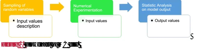
The steps of MC are summarized in Figure 1. In first step, MC generates random variables which are
[image:1.595.116.525.630.729.2]distributed between 0 to 1. The significance of this distribution is that they can be formed into actual val-ues which shape distribution of the purpose. The second step is to estimate the performance. The last step
https://doi.org/10.4236/ns.2017.912039 413 Natural Science is carried out to characterize the output values.
Statistical evaluation is vital method in which to determine the validity of measurements. It also pro-vides meaning of reported numbers and grants scientists senses to draw discussion and conclusion from their obtained numbers and variables. Luckily, most of articles dealing with applied sciences pay more at-tention to statistical methods to enhance statistical validity as proven evidence of their theory. Nowadays, advanced statistical software opens the appetite for more movement towards statistical techniques. Never-theless, inappropriate understanding of these statistical packages can lead to misinterpretation of the re-ported data [5].
Statistical methods developed to carry out statistical analysis can be broken into two categorizes: the first is so-called parametric method and the second one is non-parametric. The parametric methods are based on one assumption which is normal (homogeneous and independent) distribution of the reported
data. However, most of scientific data are violated this assumption [3].
Mood’s test is rarely used in literature for chemical data but is mostly clinical studies. Many non-pa-
rametric tests depend on Mood’s test [4]. The median test is very important quantification of studying
distribution owing to normal skewness. For instance, if variables are shared in their median then their me-dians can be comparable.
Using Mood’s Median Test, the obtained results listed in Table 1 except Fe and Mn were not
in-cluded in the Mood’s test, one can end-up with precise conclusion. Thus, the chemical data calculations were performed to answer whether MC is applicable with other non-parametric tests e.g. Kruskal-Wallis. The MC results are discussed with more emphasized on matching between these performed tests.
2. RESULTS
In Table 2, the mood’s test of the chemical data are listed. Almost half of the test was above the
me-dian and the other half was less than the meme-dian. All the meme-dian values of elements were located within upper and lower confidence intervals. For instance, for chromium the upper median was 28.11 ppm whe-reas the lower median was 18.4 ppm. The median for chromium was 22.11 ppm. Another example, for major element, e.g. iron, not reported here, the median was away from the upper and lower confidence intervals, thus, it was decided to removed from the list because only trace levels were part of this investiga-tion.
In Kruskal-Wallis Test each group of elements was treated as independent unit. It should be noted that the Kruskal-Wallis test merely informs us that the groups differ in some way. In this case, the degree of freedom was above 5, thus we cannot use critical values of Kruskal-Wallis table. It was at 0.05 signific-ance level. We can only use Chi tables. We are going to inspect each group medians to decide precisely
how they differ rather giving two examples and later visualizing them in one figure. In Table 3, it showed
the performance of Kruskal-Wallis Test for the study materials. The lowest score given by Kruskal-Wallis Test was for cadmium with z-values of −3.5 while the highest score was given to vanadium with z-value of 4.8. Thus, the data obviously have big different and the population medians of the chemical data were not all equal. The observations of median values of the study materials can easily recognize the median of easy element located between the lower and upper intervals. For example, let’s take zinc element, the lower lim-it of median was 19 ppm whereas the upper limlim-it of median was 23.7 ppm. Fortunately, all the both-side tailings were near to zero which indicated the distributions were con dent. The test statistic for the Kruskal
Wallis test is denoted H0. The calculated H0 (as Chi-Square) was 162 and medians for all reported elements
were more than H0 indicating the original data can be tested as non-parametric. So, we can conclude that
there is a difference of original data
The Nonparametric Runs Test was performed for the chemical data as listed in Table 4 as supportive
https://doi.org/10.4236/ns.2017.912039 414 Natural Science
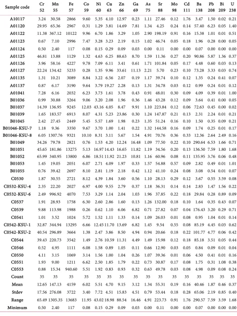
Table 1. Elemental analysis and statistical evaluation for chemical data of the study materials.
Sample code Cr 52 Mn 55 Fe 57 Co 59 Ni 60 Cu 63 Zn 66 Ga 69 As 75 88 Sr Mo 98 111 Cd 138 Ba 208 Pb 209 Bi 238 U
A10117 3.24 30.58 2866 9.60 5.35 4.10 12.97 0.23 1.11 27.46 0.12 1.76 3.47 1.50 0.02 0.21
A01120 29.95 65.36 2967 0.31 1.29 3.81 14.69 7.81 1.34 4.25 0.24 0.14 57.40 6.23 0.05 1.40
A01122 11.38 367.12 10122 9.96 6.70 1.86 3.29 1.05 2.90 198.19 0.91 0.16 15.38 1.01 0.01 0.51
A01123 0.67 7.10 2996 7.47 3.28 3.23 2.19 0.15 1.02 46.74 0.05 0.18 1.96 0.28 0.00 0.05
A01124 0.50 2.40 117 0.08 0.15 0.29 0.09 0.03 0.00 0.11 0.00 0.00 0.07 0.00 0.00 0.00
A01125 46.81 13.88 1129 1.32 4.63 6.25 88.63 8.70 1.59 11.36 0.27 0.20 90.86 5.87 1.36 0.37
A01126 3.96 58.16 4227 9.78 7.09 6.11 3.41 0.61 1.71 101.84 0.05 0.17 4.48 0.60 0.03 0.13
A01127 22.24 134.42 5233 0.28 1.35 9.96 33.61 11.13 2.21 5.70 0.23 0.10 73.28 3.33 0.03 0.74
A01135 1.31 10.21 3089 8.84 3.22 6.56 2.07 0.19 1.17 39.74 0.10 0.12 1.35 0.24 0.41 0.07
A01137 0.87 6.17 3190 9.64 3.79 19.27 2.28 0.13 1.31 34.78 0.03 0.12 0.99 0.24 0.01 0.12
A01041 7.28 6.16 2032 6.23 3.73 1.61 3.78 0.43 0.91 48.01 0.30 0.09 4.09 0.39 0.01 1.00
B01036 0.99 30.88 3264 9.06 3.20 2.08 1.96 0.36 1.46 43.28 0.12 0.09 3.64 0.41 0.00 0.05
B01037 14.39 136.95 9245 12.03 43.16 4.05 8.47 9.91 1.10 223.84 0.12 0.06 72.63 0.45 0.00 0.02
B01039 1.65 183.57 6913 8.07 4.31 5.23 23.86 0.30 1.24 147.87 0.21 0.13 2.31 2.24 0.01 0.21
B01045 2.42 27.45 2449 5.45 5.57 1.69 1.98 0.23 1.35 51.24 0.16 0.10 1.50 0.35 0.09 0.21
B01046-KSU-7 1.18 9.36 3350 9.67 3.70 1.00 1.41 0.22 1.32 144.58 0.16 0.09 1.74 0.25 0.01 0.17
B01046-KSU-8 6.05 1307.76 9321 10.10 8.31 3.11 5.67 1.54 4.91 70.76 0.36 0.33 12.36 2.64 2.49 0.16
B01049 34.26 79.78 2821 0.76 1.53 4.20 12.24 16.48 1.09 77.50 0.22 0.10 290.64 6.53 1.66 0.71
B01051 45.65 181.86 13275 5.13 16.97 14.43 16.65 11.82 1.19 34.56 0.20 0.13 136.50 7.59 1.80 1.68 B01052 65.99 340.95 13800 6.86 18.51 11.92 21.23 10.81 1.16 60.96 0.08 0.11 135.95 3.76 0.06 0.48
B01053 1.45 19.05 2051 6.07 2.71 4.09 1.97 0.33 1.57 54.88 0.57 0.09 2.82 0.49 0.01 1.01
B01055 0.76 39.42 2697 8.10 2.81 1.19 2.18 0.42 1.12 41.10 0.24 0.08 3.08 0.54 0.01 0.07
C0530 1.87 30.55 2721 8.12 4.39 1.84 3.60 0.56 1.10 28.13 0.29 0.12 3.67 0.55 3.59 0.08
C0532-KSU-4 2.35 22.20 2027 6.97 4.00 9.55 2.79 0.37 1.18 36.31 0.14 0.14 2.83 1.47 1.56 0.22
C0532-KSU-6 2.49 996.92 4070 7.53 3.29 1.14 2.04 1.03 1.96 37.85 0.22 0.18 29.84 0.28 0.89 0.09
C0537 1.91 28.93 1758 6.30 2.60 2.86 1.60 0.13 1.26 132.00 0.18 0.10 1.64 0.35 0.43 0.07
C0539 9.88 113.98 1988 0.26 0.62 1.10 6.06 6.82 0.71 27.82 0.07 0.04 176.43 3.20 0.29 0.71
C0541 1.01 3.52 1024 5.72 1.52 1.11 1.33 0.14 1.09 26.03 0.01 0.08 0.95 1.04 0.01 0.14
C0542-KSU-1 32.87 344.94 13295 6.66 12.45 11.70 13.69 6.82 1.45 9.54 0.55 0.08 85.19 4.45 0.03 0.62 C0542-KSU-2 40.54 296.89 3664 1.38 2.47 3.86 8.50 4.94 0.94 20.66 0.18 0.22 101.77 4.77 0.06 0.42
C0544 39.43 220.73 3542 1.49 2.76 10.59 11.31 4.49 1.49 15.98 0.12 0.18 85.18 3.51 0.05 0.44
C0546 0.52 4.95 1111 6.08 1.58 0.89 1.05 0.11 0.66 12.90 0.03 0.05 0.84 0.09 0.01 0.04
C0550 4.11 3.15 1069 3.14 1.56 1.00 1.04 0.26 1.07 39.36 0.01 0.06 4.50 0.41 0.01 0.16
C0551 1.93 9.00 1211 6.62 2.50 1.85 1.79 0.22 0.73 30.87 0.17 0.08 1.75 0.31 1.08 0.38
C0553 0.88 15.34 940.60 5.51 1.92 0.83 0.93 0.32 0.63 49.78 0.03 0.08 4.98 0.09 0.08 0.24
Count 35 35 35 35 35 35 35 35 35 35 35 35 35 35 35 35
Mean 12.65 147.13 4159 6.02 5.51 4.70 9.15 3.12 1.34 55.31 0.19 0.16 40.46 1.87 0.46 0.37
Stdev 17.56 276.08 3722 3.40 7.72 4.51 15.83 4.51 0.79 53.44 0.18 0.28 65.06 2.19 0.85 0.40
Range 65.49 1305.35 13683 11.95 43.02 18.98 88.54 16.46 4.91 223.73 0.91 1.76 290.57 7.59 3.59 1.68
https://doi.org/10.4236/ns.2017.912039 415 Natural Science Continued
25th Percentile
(Q1) 1.18 9.36 1988 3.14 1.92 1.19 1.96 0.22 1.07 26.03 0.07 0.08 1.75 0.31 0.01 0.08
50th Percentile
(Median) 2.49 30.58 2967 6.62 3.28 3.23 3.29 0.42 1.18 39.36 0.16 0.10 4.09 0.55 0.03 0.21
75th Percentile
(Q3) 22.24 181.86 4227 8.84 5.35 6.25 12.24 6.82 1.46 60.96 0.24 0.16 73.28 3.33 0.43 0.51
Maximum 65.99 1307.76 13800 12.03 43.16 19.27 88.63 16.48 4.91 223.84 0.91 1.76 290.64 7.59 3.59 1.68
95.0% CI Mean 6.62 to 18.652.2 to 2,412,880 to 5438 4.8 to 7.2 2.86 to 8.163.15 to 6.23.72 to 14.591.5 to 4.661.07 to 1.6136.9 to 73.70.13 to 0.250.07 to 0.2618.1 to 62.8 1.1 to 2.60.17 to 0.750.23 to 0.51
95.0% CI Sigma 14.2 to 23.0223 to 3,613,010 to 48,772.75 to 4.466.24 to 10.123.64 to 5.912.8 to 20.7 3.6 to 5.90.63 to 1.0343.3 to 70.020.15 to 0.240.23 to 0.3752.62 to 85.21.76 to 2.80.68 to 1.110.32 to 0.53 Anderson-Darling
Normality Test 4.26 5.44 3.190 1.08 5.22 2.26 5.02 4.58 3.04 2.79 1.90 8.10 4.37 3.11 5.59 2.34
P-Value
(A-D Test) 0.00 0.00 0.0000 0.01 0.00 0.00 0.00 0.00 0.00 0.00 0.00 0.00 0.00 0.00 0.00 0.00
Skewness 1.52 3.20 1.574 −0.48 3.83 1.56 4.05 1.43 2.94 1.81 2.23 5.52 2.19 1.26 2.24 1.72
P-Value
(Skewness) 0.00 0.00 0.0007 0.21 0.00 0.00 0.00 0.00 0.00 0.00 0.00 0.00 0.00 0.00 0.00 0.00
Kurtosis 1.36 10.90 1.499 −0.82 17.07 2.17 19.30 1.02 12.37 2.91 6.60 31.73 5.53 0.43 5.03 2.84 P-Value
(Kurtosis) 0.11 0.00 0.0933 0.18 0.00 0.04 0.00 0.19 0.00 0.01 0.00 0.00 0.00 0.45 0.00 0.02
Table 2. Mood’s median test for the study materials. Mood’s Median-Monte Carlo: U 238
Test Information
H0: Median 1 = Median 2 = … = Median k Ha: At least one pair Median i Median j
Results: 51 V Cr 52 Co 59 Ni 60 Cu 63 Zn 66 Ga 69 As 75 Sr 88 Mo 98 111 Cd 130 Te 138 Ba 205 Tl 208 Pb 209 Bi 238 U Count (N ≤ Overall
Median) 0 1 10 1 0 0 8 0 0 11 11 11 0 11 11 8 11
Count (N > Overall
Median) 11 10 1 10 11 11 3 11 11 0 0 0 11 0 0 3 0
Median 69.07 22.10 5.71 14.80 37.57 19.10 8.59 27.56 60.17 5.29 1.04 0.04 45.46 0.04 4.25 0.30 1.60 UC Median (2-sided,
95% approx.) 82.16 28.11 8.13 17.79 51.68 23.76 9.89 37.24 187.31 7.04 1.51 0.06 59.41 0.06 5.46 37.01 1.82 LC Median (2-sided,
95% approx.) 55.71 18.38 4.80 12.29 29.78 15.40 6.97 18.56 35.92 3.77 0.65 0.04 30.55 0.04 3.95 0.16 1.24 Overall Median 9.849
Chi-Square 158.64
DF 16
Monte Carlo P-Value
(2-sided) 0.0000
Monte Carlo P-Value
99% CI Upper 0.0000
Monte Carlo P-Value
https://doi.org/10.4236/ns.2017.912039 418 Natural Science support our hypothesis of difference between the variables.
Matrix correlations were studied for the study chemical using Pearson Methods as listed in Table 5.
Arsenic was almost correlated with all elements.
3. CONCLUSION
As seen in result section, Monte Carlo simulation showed clear difference at significant level of 95%
among the study data. The difference of the reported data makes the non-parametric test valid. The Figure
2, log scale, illustrated the significant difference in the reported data. To support the Monte Carlo
[image:7.595.64.532.222.475.2]simula-tion, Kruskal-Wall test in Figure 3 showed the significant difference among median variables. At 95%
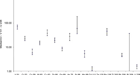
Figure 2. Medians (log scale) of the study materials for mood’s median test.
[image:7.595.63.536.522.711.2]https://doi.org/10.4236/ns.2017.912039 419 Natural Science
Table 5. Correlation calculations between chemical and radiation measurements using pearson me-thods for adhesive materials.
Pearson
Correlations V 51 Cr 52 Co 59 Ni 60 Cu 63 Zn 66 Ga 69 As 75 Sr 88 Mo 98 Cd 111 Ba 138 Pb 208 U 238
V 51 1 0.8760 0.7750 0.8310 0.5657 0.5150 0.5226 0.7542 −0.3594 0.1520 0.2643 0.2938 0.3885 0.6338
Cr 52 1 0.8497 0.9131 0.7277 0.6793 0.7778 0.8411 −0.2014 0.2396 0.3863 0.5029 0.4371 0.4608
Co 59 1 0.6871 0.5913 0.4029 0.7719 0.7406 0.1103 −0.0366 0.0353 0.3864 0.2491 0.3372
Ni 60 1 0.7296 0.6306 0.6703 0.8673 −0.3837 0.3910 0.5516 0.4769 0.3896 0.3355
Cu 63 1 0.5413 0.9020 0.9206 0.1427 0.7565 0.7535 0.5898 0.5024 −0.0918
Zn 66 1 0.6165 0.4656 0.0334 0.4472 0.6353 0.8333 0.8842 0.3295
Ga 69 1 0.8363 0.3635 0.5006 0.5395 0.7060 0.5255 −0.0540
As 75 1 −0.0479 0.5283 0.5985 0.5103 0.3535 0.1042
Sr 88 1 0.0759 −0.0212 0.3956 0.2847 −0.4002
Mo 98 1 0.9293 0.4730 0.5549 −0.3364
Cd 111 1 0.6580 0.6371 −0.1757
Ba 138 1 0.7936 −0.0433
Pb 208 1 0.2459
U 238 1
Pearson
Probabilities V 51 Cr 52 Co 59 Ni 60 Cu 63 Zn 66 Ga 69 As 75 Sr 88 Mo 98 Cd 111 Ba 138 Pb 208 U 238
V 51 0.0004 0.0051 0.0015 0.0697 0.1050 0.0991 0.0073 0.2777 0.6555 0.4322 0.3806 0.2377 0.0363
Cr 52 0.0009 0.0001 0.0111 0.0215 0.0048 0.0012 0.5526 0.4780 0.2406 0.1148 0.1789 0.1538
Co 59 0.0195 0.0554 0.2192 0.0054 0.0091 0.7468 0.9149 0.9179 0.2405 0.4600 0.3105
Ni 60 0.0108 0.0375 0.0240 0.0005 0.2441 0.2345 0.0786 0.1381 0.2362 0.3131
Cu 63 0.0855 0.0001 0.0001 0.6755 0.0070 0.0074 0.0561 0.1153 0.7884
Zn 66 0.0434 0.1490 0.9223 0.1678 0.0357 0.0014 0.0003 0.3225
Ga 69 0.0013 0.2719 0.1168 0.0867 0.0152 0.0969 0.8748
As 75 0.8888 0.0948 0.0517 0.1087 0.2863 0.7605
Sr 88 0.8246 0.9508 0.2285 0.3961 0.2227
Mo 98 0.0000 0.1417 0.0764 0.3118
Cd 111 0.0277 0.0350 0.6054
Ba 138 0.0035 0.8995
Pb 208 0.4662
U 238
significance level, we conclude that the study data were non-identical populations.
REFERENCES
https://doi.org/10.4236/ns.2017.912039 420 Natural Science Building Materials Used in Saudi Arabia. Journal of Fundamental and Applied Sciences, 9, 1341-1348.
2. Landau, D.P. and Binder, K. (2014) A Guide to Monte Carlo Simulations in Statistical Physics. Cambridge Uni-versity Press, Cambridge.
3. Derrac, J., et al. (2011) A Practical Tutorial on the Use of Nonparametric Statistical Tests as a Methodology for Comparing Evolutionary and Swarm Intelligence Algorithms. Swarm and Evolutionary Computation, 1, 3-18. https://doi.org/10.1016/j.swevo.2011.02.002
4. Chen, Z. and Zhang, G. (2016) Comparing Survival Curves Based on Medians. BMC Medical Research Metho-dology, 16, 33. https://doi.org/10.1186/s12874-016-0133-3