Structuring Knowledge for Reference Generation:
A Clustering Algorithm
Albert Gatt
Department of Computing Science
University of Aberdeen
Scotland, United Kingdom
[email protected]
Abstract
This paper discusses two problems that arise in the Generation of Referring Expressions: (a) numeric-valued attributes, such as size or location; (b) perspective-taking in reference. Both problems, it is argued, can be resolved if some structure is imposed on the available knowledge prior to content determination. We describe a clustering algorithm which is suffi-ciently general to be applied to these diverse problems, discuss its application, and evaluate its performance.
1
Introduction
The problem of Generating Referring Expressions (GRE) can be summed up as a search for the prop-erties in a knowledge base (KB) whose combination uniquely distinguishes a set of referents from their dis-tractors. The content determination strategy adopted in such algorithms is usually based on the assump-tion (made explicit in Reiter (1990)) that the space of possible descriptions is partially ordered with respect to some principle(s) which determine their adequacy. Traditionally, these principles have been defined via an interpretation of the Gricean maxims (Dale, 1989; Reiter, 1990; Dale and Reiter, 1995; van Deemter, 2002)1. However, little attention has been paid to con-textual or intentional influences on attribute selection (but cf. Jordan and Walker (2000); Krahmer and The-une (2002)). Furthermore, it is often assumed that all relevant knowledge about domain objects is repre-sented in the database in a format (e.g. attribute-value pairs) that requires no further processing.
This paper is concerned with two scenarios which raise problems for such an approach to GRE:
1. Real-valued attributes, e.g. size or spatial coor-dinates, which represent continuous dimensions. The utility of such attributes depends on whether a set of referents have values that are ‘sufficiently
1
For example, the Gricean Brevity maxim (Grice, 1975) has been interpreted as a directive to find the shortest possible description for a given referent
close’ on the given dimension, and ‘sufficiently distant’ from those of their distractors. We dis-cuss this problem in§2.
2. Perspective-taking The contextual appropriate-ness of a description depends on the perspective being taken in context. For instance, if it is known of a referent that it is ateacher, and asportsman, it is better to talk ofthe teacherin a context where another referent has been introduced as the stu-dent. This is discussed further in§3.
Our aim is to motivate an approach to GRE where these problems are solved by pre-processing the infor-mation in the knowledge base, prior to content deter-mination. To this end,§4 describes a clustering algo-rithm and shows how it can be applied to these different problems to structure the KB prior to GRE.
2
Numeric values: The case of location
Several types of information about domain entities, such as gradable properties (van Deemter, 2000) and physical location, are best captured by real-valued at-tributes. Here, we focus on the example of location as an attribute taking a tuple of values which jointly de-termine the position of an entity.
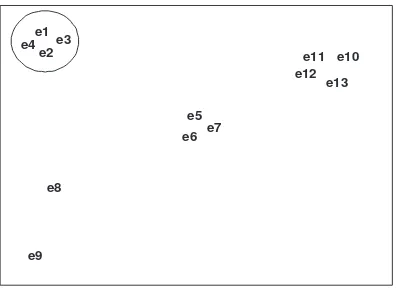
The ability to distinguish groups is a well-established feature of the human perceptual appara-tus (Wertheimer, 1938; Treisman, 1982). Representing salient groups can facilitate the task of excluding dis-tractors in the search for a referent. For instance, the set of referents marked as the intended referential tar-get in Figure 1 is easily distinguishable as a group and warrants the use of a spatial description such asthe ob-jects in the top left corner, possibly with a collective predicate, such as clustered or gathered. In case of reference to a subset of the marked set, although loca-tion would be insufficient to distinguish the targets, it would reduce the distractor set and facilitate reference resolution2.
In GRE, an approach to spatial reference based on grouping has been proposed by Funakoshi et al.
2
e1 e4 e3
e2
e8
e9
e13 e12
e10 e11
[image:2.595.82.281.70.215.2]e6 e7 e5
Figure 1: Spatial Example
(2004). Given a domain and a target referent, a se-quence of groups is constructed, starting from the largest group containing the referent, and recursively narrowing down the group until only the referent is identified. The entire sequence is then rendered lin-guistically. The algorithm used for identifying percep-tual groups is the one proposed by Thorisson (1994), the core of which is a procedure which takes as input a list of pairs of objects, ordered by the distance be-tween the entities in the pairs. The procedure loops through the list, finding the greatest difference in dis-tance between two adjacent pairs. This is determined as a cutoff point for group formation. Two problems are raised by this approach:
P1 Ambiguous clusters A domain entity can be placed in more than one group. If, say, the in-put list is
{a, b},{c, e},{a, f}
and the great-est difference after the first iteration is between
{c, e}and{a, f}, then the first group to be formed will be{a, b, c, e}with{a, f}likely to be placed in a different group after further iterations. This may be confusing from a referential point of view. The problem arises because grouping or cluster-ing takes place on the basis ofpairwise proxim-ity or distance. This problem can be partially cir-cumvented by identifying groups on several per-ceptual dimensions (e.g. spatial distance, colour, and shape) and then seeking to merge identical groups determined on the basis of these differ-ent qualities (see Thorisson (1994)). However, the grouping strategy can still return groups which do not conform to human perceptual principles. A better strategy is to base clustering on the Near-est Neighbour Principle, familiar from computa-tional geometry (Prepaarata and Shamos, 1985), whereby elements are clustered with their nearest neighbours, given a distance function. The solu-tion offered below is based on this principle.
P2 Perceptual proximity Absolute distance is not
sufficient for cluster identification. In Figure 1, for example, the pairs{e1, e2}and{e5, e6}could easily be consecutively ranked, since the distance between e1 and e2 is roughly equal to that be-tweene5ande6. However, they would not natu-rally be clustered together by a human observer, because grouping of objects also needs to take into account the position of the surrounding ele-ments. Thus, whilee1is as far away frome2as
e5is frome6, there are elements which are closer to{e1, e2}than to{e5, e6}.
The proposal in §4 represents a way of getting around these problems, which are expected to arise in any kind of domain where the information given is the pairwise distance between elements. Before turning to the framework, we consider another situation in GRE where the need for clustering could arise.
3
Perspectives and semantic similarity
In real-world discourse, entities can often be talked about from different points of view, with speakers bringing to bear world and domain-specific knowledge to select information that is relevant to the current topic. In order to generate coherent discourse, a gener-ator should ideally keep track of how entities have been referred to, and maintain consistency as far as possible.
type profession nationality
e1 man student englishman
e2 woman teacher italian
e3 man chef greek
Table 1: Semantic Example
Supposee1 in Table 1 has been introduced into the discourse via the descriptionthe student and the next utterance requires a reference toe2. Any one of the three available attributes would suffice to distinguish the latter. However, a description such asthe woman orthe italianwould describe this entity from a different point of view relative toe1. By hypothesis,the teacher is more appropriate, because the property ascribed to
e2is more similar to that ascribed toe1.
[image:2.595.324.502.414.467.2]and the cheffor{e1, e3}is relatively odd compared to the alternativethe englishman and the greek. In both kinds of scenarios, a GRE algorithm that relied on a rigid preference order could not guarantee that a coher-ent description would be generated every time it was available.
The issues raised here have never been systemati-cally addressed in the GRE literature, although support for the underlying intuitions can be found in various quarters. Kronfeld (1989) distinguishes between func-tionallyandconversationallyrelevant descriptions. A description is functionally relevant if it succeeds in dis-tinguishing the intended referent(s), but conversational relevance arises in part from implicatures carried by the use of attributes in context. For example, describ-inge1asthe studentcarries the (Gricean) implicature that the entity’s academic role or profession is some-how relevant to the current discourse. When two enti-ties are described using contrasting properenti-ties, saythe student and the italian, the listener may find it harder to work out the relevance of the contrast. In a related vein, Aloni (2002) formalises the appropriateness of an answer to a question of the formWh x?with reference to the ‘conceptual covers’ or perspectives under which xcan be conceptualised, not all of which are equally relevant given the hearer’s information state and the discourse context.
With respect to plurals, Eschenbachet al.(1989) ar-gue that the generation of a plural anaphor with a split antecedent is more felicitous when the antecedents have something in common, such as their ontological category. This constraint has been shown to hold psy-cholinguistically (Kaup et al., 2002; Koh and Clifton, 2002; Moxey et al., 2004). Gatt and van Deemter (2005a) have shown that people’s perception of the ad-equacy of plural descriptions of the form,theN1and (the) N2 is significantly correlated with the seman-tic similarity of N1 and N2, while singular descrip-tions are more likely to be aggregated into a plural if semantically similar attributes are available (Gatt and Van Deemter, 2005b).
The two kinds of problems discussed here could be resolved by pre-processing the KB in order to iden-tify available perspectives. One way of doing this is to group available properties into clusters of seman-tically similar ones. This requires a well-defined no-tion of ‘similarity’ which determines the ‘distance’ be-tween properties in semantic space. As with spatial clustering, the problem is then of how to get from pairwise distance to well-formed clusters or groups, while respecting the principles underlying human per-ceptual/conceptual organisation. The next section de-scribes an algorithm that aims to achieve this.
4
A framework for clustering
In what follows, we assume the existence of a set of clustersCin a domainSof objects (entities or proper-ties), to be ‘discovered’ by the algorithm. We further assume the existence of a dimension, which is char-acterised by a functionδthat returns the pairwise dis-tanceδ(a, b), whereha, bi ∈S×S. In case an attribute is characterised by more than one dimension, sayhx, yi
coordinates in a 2D plane, as in Figure 1, thenδis de-fined as the Euclidean distance between pairs:
δ=
s X
hx,yi∈D
|xab−yab|2 (1)
whereDis a tuple of dimensions,xab=δ(a, b)on di-mensionx. δsatisfies the axioms ofminimality(2a), symmetry (2b), and the triangle inequality (2c), by which it determines a metric space onS:
δ(a, b)≥0∧ δ(a, b) = 0↔a=b
(2a)
δ(a, b) =δ(b, a) (2b)
δ(a, b) +δ(b, c)≥δ(a, c) (2c)
We now turn to the problems raised in§2. P1 would be avoided by a clustering algorithm that satisfies (3).
\
Ci∈C
=∅ (3)
It was also suggested above that a potential solution to P1 is to cluster using the Nearest Neighbour Princi-ple. Before considering a solution to P2, i.e. the prob-lem of discovering clusters that approximate human intuitions, it is useful to recapitulate the classic prin-ciples of perceptual grouping proposed by Wertheimer (1938), of which the following two are the most rele-vant:
1. Proximity The smaller the distance between ob-jects in the cluster, the more easily perceived it is.
2. Similarity Similar entities will tend to be more easily perceived as a coherent group.
Arguably, once a numeric definition of (semantic) similarity is available, the Similarity Principle boils down to the Proximity principle, where proximity is defined via a semantic distance function. This view is adopted here. How well our interpretation of these principles can be ported to the semantic clustering problem of §3 will be seen in the following subsec-tions.
proximity (resp. distance) of a pairha, biis contingent not only onδ(a, b), but also on the distance ofaand
b from all other elements in S. A first step towards meeting this requirement is to consider, for a given pair of objects, not only the absolute distance (prox-imity) between them, but also the extent to which they are equidistant from other objects inS. Formally, a measure of perceived proximityprox(a, b)can be ap-proximated by the following function. Let the two sets
Pab, Dabbe defined as follows:
Pab=x|x∈S∧δ(x, a)∼δ(x, b)
Dab=
y|y∈S∧δ(y, a)6∼δ(y, b)
Then:
prox(a, b) =F(δ(a, b),|Pab|,|Dab|) (4)
that is,prox(a, b)is a function of the absolute dis-tanceδ(a, b), the number of elements in S − {a, b}
which are roughly equidistant from aandb, and the number of elements which are not equidistant. One way of conceptualising this is to consider, for a given objecta, the list of all other elements ofS, ranked by their distance (proximity) toa. Suppose there exists an objectbwhose ranked list is similar to that ofa, while another objectc’s list is very different. Then, all other things being equal (in particular, the pairwise absolute distance),aclusters closer tobthan doesc.
This takes us from a metric, distance-based concep-tion, to a broader notion of the ‘similarity’ between two objects in a metric space. Our definition is inspired by Tversky’s feature-based Contrast Model (1977), in which the similarity of a, bwith feature setsA, B is a linear function of the features they have in com-mon and the features that pertain only toAorB, i.e.:
sim(a, b) = f(A∩B)−f(A∩B). In (4), the dis-tance ofaandbfrom every other object is the relevant feature.
4.1 Computing perceived proximity
The computation of pairwise perceived proximity
prox(a, b), shown in Algorithm 1, is the first step to-wards finding clusters in the domain.
Following Thorisson (1994), the procedure uses the absolute distanceδto calculate ‘absolute proxim-ity’ (1.7), a value in(0,1), with1 corresponding to
δ(a, b) = 0, i.e. identity (cf. axiom (2a) ). The proce-dure then visits each element of the domain, and com-pares its rank with respect toaandb(1.9–1.13)3, in-crementing a proximity scores(1.10) if the ranks are
3
We simplify the presentation by assuming the function
rank(x, a)that returns the rank ofxwith respect toa. In practice, this is achieved by creating, for each element of the input pair, a totally ordered listLasuch thatLa[r]holds the
set of elements ranked atrwith respect toδ(x, a)
Algorithm 1prox(a,b)
Require: δ(a, b) Require: k(a constant)
1: maxD←maxhx,yi∈S×Sδ(x, y)
2: if a=b then
3: return 1
4: end if
5: s←0
6: d←0
7: p(a, b)←1−maxDδ(a,b)
8: for all x∈S− {a, b} do
9: if |rank(x, a)−rank(x, b)| ≤k then
10: s←s+ 1
11: else
12: d←d+ 1
13: end if
14: end for
15: return p(a, b)×s d
approximately equal, or a distance score dotherwise (1.12). Approximate equality is determined via a con-stantk(1.1), which, based on our experiments is set to a tenth the size ofS. The procedure returns the ratio of proximity and distance scores, weighted by the abso-lute proximityp(a, b)(1.15). Algorithm 1 is called for all pairs inS×S yielding, for each elementa∈S, a list of elements ordered by their perceived proximity to
a. The entity with the highest proximity toais called itsanchor. Note that any domain object has one, and only one anchor.
4.2 Creating clusters
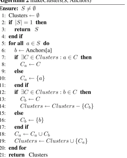
The procedure makeClusters(S, Anchors), shown in its basic form in Algorithm 2, uses the notion of an anchor introduced above. The rationale behind the algorithm is captured by the following declarative principle, whereC ∈ Cis any cluster, and
anchor(a, b)means ‘bis the anchor ofa’:
a∈C∧anchor(a, b)→b∈C (5)
A cluster is defined as the transitive closure of the anchor relation, that is, if it holds that anchor(a, b)
and anchor(b, c), then{a, b, c} will be clustered to-gether. Apart from satisfying (5), the procedure also in-duces a partition onS, satisfying (3). Given these pri-mary aims, no attempt is made, once clusters are gen-erated, to further sub-divide them, although we briefly return to this issue in§5. The algorithm initialises a setClustersto empty (2.1), and iterates through the list of objectsS(2.5). For each objectaand its anchor
Algorithm 2makeClusters(S, Anchors)
Ensure: S6=∅
1: Clusters← ∅
2: if |S|= 1 then
3: return S
4: end if
5: for all a∈S do
6: b←Anchors[a]
7: if ∃C∈Clusters:a∈C then
8: Ca←C
9: else
10: Ca← {a}
11: end if
12: if ∃C∈Clusters:b∈C then
13: Cb←C
14: Clusters←Clusters− {Cb}
15: else
16: Cb← {b}
17: end if
18: Ca←Ca∪Cb
19: Clusters←Clusters∪ {Ca}
20: end for
21: return Clusters
(2.10, 2.16). The procedure simply merges the cluster containingawith that of itsb(2.18), having removed the latter from the cluster set (2.14).
This algorithm is guaranteed to induce a partition, since no element will end up in more than one group. It does not depend on an ordering of pairs `a la Tho-risson. However, problems arise when elements and anchors are clustered n¨aively. For instance, if an el-ement is very distant from every other elel-ement in the domain,prox(a, b)will still find an anchor for it, and
makeClusters(S, Anchors)will place it in the same cluster as its anchor, although it is an outlier. Before describing how this problem is rectified, we introduce the notion of afamily(F) of elements. Informally, this is a set of elements ofSthat have the same anchor, that is:
∀a, b∈F:anchor(a, x)∧anchor(b, y)↔x=y
(6) The solution to the outlier problem is to calculate a centroid valuefor each family found afterprox(a, b). This is the average proximity between the common an-chor and all members of its family, minus one stan-dard deviation. Prior to merging, at line (2.18), the algorithm now checks whether the proximity value be-tween an element and its anchor falls below the cen-troid value. If it does, the the cluster containing an object and that containing its anchor are not merged.
4.3 Two applications
The algorithm was applied to the two scenarios de-scribed in §2 and §3. In the spatial domain, the al-gorithm returns groups or clusters of entities, based on their spatial proximity. This was tested on domains like Figure 1 in which the input is a set of entities whose position is defined as a pair of x/y coordinates. Fig-ure 1 illustrates a potential problem with the proce-dure. In that figure, it holds thatanchor(e8, e9)and
anchor(e9, e8), makinge8 ande9 a reciprocal pair. In such cases, the algorithm inevitably groups the two elements, whatever their proximity/distance. This may be problematic when elements of a reciprocal pair are very distant from eachother, in which case they are un-likely to be perceived as a group. We return to this problem briefly in§5.
The second domain of application is the cluster-ing of properties into ‘perspectives’. Here, we use the information-theoretic definition of similarity de-veloped by Lin (1998) and applied to corpus data by Kilgarriff and Tugwell (Kilgarriff and Tugwell, 2001). This measure defines the similarity of two words as a function of the likelihood of their occurring in the same grammatical environments in a corpus. This measure was shown experimentally to correlate highly with hu-man acceptability judgments of disjunctive plural de-scriptions (Gatt and van Deemter, 2005a), when com-pared with a number of measures that calculate the similarity of word senses in WordNet. Using this as the measure of semantic distance between words, the algorithm returns clusters such as those in Figure 2.
input: {waiter, essay, footballer, article, servant, cricketer, novel, cook, book, maid, player, striker, goalkeeper}
output:
1 {essay, article, novel, book}
2 {footballer, cricketer}
3 {waiter, cook, servant, maid}
[image:5.595.74.293.78.349.2]4 {player, goalkeeper, striker}
Figure 2: Output on a Semantic Domain
spatial semantic
1 0.94 0.58
2 0.86 0.36
3 0.62 0.76
4 0.93 0.52
[image:6.595.116.246.69.148.2]mean 0.84 0.64
Table 2: Proportion of agreement among participants
in GRE are not words but ‘properties’ (e.g. values of attributes) which can be realised in a number of differ-ent ways (if, for instance, there are a number of syn-onyms corresponding roughly to the same intension). This could be remedied by defining similarity as ‘dis-tance in an ontology’; conversely, properties could be viewed as a set of potential (word) realisations.
5
Evaluation
The evaluation of the algorithm was based on a com-parison of its output against the output of human beings in a similar task.
Thirteen native or fluent speakers of English volun-teered to participate in the study. The materials con-sisted of 8 domains, 4 of which were graphical repre-sentations of a 2D spatial layout containing 13 points. The pictures were generated by plotting numerical x/y coordinates (the same values are used as input to the algorithm). The other four domains consisted of a set of 13 arbitrarily chosen nouns. Participants were presented with an eight-page booklet with spatial and semantic domains on alternate pages. They were in-structed to draw circles around the best clusters in the pictures, or write down the words in groups that were related according to their intuitions. Clusters could be of arbitrary size, but each element had to be placed in exactly one cluster.
5.1 Participant agreement
Participant agreement on each domain was measured using kappa. Since the task did not involve predefined clusters, the set ofuniquegroups (denotedG) gener-ated by participants in every domain was identified, representing the set of ‘categories’ available post hoc. For each domain element, the number of times it oc-curred in each group served as the basis to calculate the proportion of agreement among participants for the element. The total agreementP(A)and the agreement expected by chance,P(E)were then used in the stan-dard formula
k= P(A)−P(E) 1−P(E)
Table 2 shows a remarkable difference between the two domain types, with very high agreement on spa-tial domains and lower values on the semantic task.
The difference was significant (t = 2.54,p < 0.05). Disagreement on spatial domains was mostly due to the problem of reciprocal pairs, where participants dis-agreed on whether entities such ase8ande9in Figure 1 gave rise to a well-formed cluster or not. However, all the participants were consistent with the version of the Nearest Neighbour Principle given in (5). If an element was grouped, it was always grouped with its anchor.
The disagreement in the semantic domains seemed to turn on two cases4:
1. Sub-clusters Whereas some proposals included clusters such as{man, woman, boy, girl, infant, toddler, baby, child} , others chose to group{
infant, toddler, baby,child} separately.
2. Polysemy For example,liver was in some cases clustered with { steak, pizza } , while others grouped it with items like{heart, lung}.
Insofar as an algorithm should capture the whole range of phenomena observed, (1) above could be accounted for by making repeated calls to the Algorithm to sub-divide clusters. One problem is that, in case only one cluster is found in the original domain, the same cluster will be returned after further attempts at sub-clustering. A possible solution to this is to redefine the parameter
kin Algorithm (1), making the condition for proximity more strict. As for the second observation, the desider-atum expressed in (3) may be too strong in the semantic domain, since words can be polysemous. As suggested above, one way to resolve this would be to measure distance between word senses, as opposed to words.
5.2 Algorithm performance
The performance of the algorithm (hereafter thetarget) against the human output was compared to two base-line algorithms. In the spatial domains, we used an implementation of the Thorisson algorithm (Thorisson, 1994) described in§2. In our implementation, the pro-cedure was called iteratively until all domain objects had been clustered in at least one group.
For the semantic domains, the baseline was a simple procedure which calculated the powerset of each do-mainS. For each subset inpow(S)− {∅, S}, the pro-cedure calculates the mean pairwise similarity between words, returning an ordered list of subsets. This partial order is then traversed, choosing subsets until all ele-ments had been grouped. This seemed to be a reason-able baseline, because it corresponds to the intuition that the ‘best cluster’ from a semantic point of view is the one with the highest pairwise similarity among its elements.
4
The output of the target and baseline algorithms was compared to human output in the following ways:
1. By item In each of the eight test domains, an agreement score was calculated for each domain elemente(i.e. 13 scores in each domain). Let
Usbe the set of distinct groups containinge pro-posed by the experimental participants, and letUa be the set of unique groups containingeproposed by the algorithm (|Ua| = 1in case of the target algorithm, but not necessarily for the baselines, since they do not impose a partition). For each pairhUai, Usjiof algorithm-human clusters, the agreement score was defined as
|Uai∩Usj|
|Uai∩Usj|+|Uai∩Usi|
,
i.e. the ratio of the number of elements on which the human/algorithm agree, and the number of el-ements on which they do not agree. This returns a number in(0,1)with1indicating perfect agree-ment. The maximal such score for each entity was selected. This controlled for the possible advan-tage that the target algorithm might have, given that it, like the human participants, partitions the domain.
2. By participantAn overall mean agreement score was computed for each participant using the above formula for the target and baseline algo-rithms in each domain.
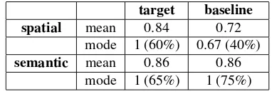
Results by itemTable 3 shows the mean and modal agreement scores obtained for both target and base-line in each domain type. At a glance, the target algo-rithm performed better than the baseline on the spatial domains, with a modal score of 1, indicating perfect agreement on 60% of the objects. The situation is dif-ferent in the semantic domains, where target and base-line performed roughly equally well; in fact, the modal score of 1 accounts for 75% baseline scores.
target baseline
spatial mean 0.84 0.72
mode 1 (60%) 0.67 (40%)
semantic mean 0.86 0.86
[image:7.595.84.275.568.634.2]mode 1 (65%) 1 (75%)
Table 3: Mean and modal agreement scores
Unsurprisingly, the difference between target and baseline algorithms was reliable on the spatial domains (t= 2.865,p < .01), but not on the semantic domains (t <1, ns). This was confirmed by a one-way Analysis of Variance (ANOVA), testing the effect of algorithm (target/baseline) and domain type (spatial/semantic) on
agreement results. There was a significant main ef-fect of domain type (F = 6.399, p = .01), while the main effect of algorithm was marginally significant (F = 3.542,p=.06). However, there was a reliable type×algorithm interaction (F = 3.624,p = .05), confirming the finding that the agreement between tar-get and human output differed between domain types. Given the relative lack of agreement between partic-ipants in the semantic clustering task, this is unsur-prising. Although the analysis focused on maximal scores obtained per entity, if participants do not agree on groupings, then the means which are statistically compared are likely to mask a significant amount of variance. We now turn to the analysis by participants.
Results by participantThe difference between tar-get and baselines in agreement across participants was significant both for spatial (t = 16.6, p < .01) and semantic (t = 5.759, t < .01) domain types. This corroborates the earlier conclusion: once par-ticipant variation is controlled for by including it in the statistical model, the differences between target and baseline show up as reliable across the board. A univariate ANOVA corroborates the results, showing no significant main effect of domain type (F < 1, ns), but a highly significant main effect of algorithm (F = 233.5, p < .01) and a significant interaction (F = 44.3,p < .01).
SummaryThe results of the evaluation are encour-aging, showing high agreement between the output of the algorithm and the output that was judged by hu-mans as most appropriate. They also suggest frame-work of§4 corresponds to human intuitions better than the baselines tested here. However, these results should be interpreted with caution in the case of semantic clus-tering, where there was significant variability in human agreement. With respect to spatial clustering, one out-standing problem is that of reciprocal pairs which are too distant from eachother to form a perceptually well-formed cluster. We are extending the empirical study to new domains involving such cases, in order to infer from the human data a threshold on pairwise distance between entities, beyond which they are not clustered.
6
Conclusions and future work
This paper attempted to achieve a dual goal. First, we highlighted a number of scenarios in which the perfor-mance of a GRE algorithm can be enhanced by an ini-tial step which identifies clusters of entities or proper-ties. Second, we described an algorithm which takes as input a set of objects and returns a set of clusters based on a calculation of theirperceived proximity. The def-inition of perceived proximity seeks to take into ac-count some of the principles of human perceptual and conceptual organisation.
two problems in GRE, namely, the generation of spatial references involving collective predicates (e.g. gath-ered), and the identification of the available perspec-tives or conceptual covers, under which referents may be described.
References
M. Aloni. 2002. Questions under cover. In D. Barker-Plummer, D. Beaver, J. van Benthem, and P. Scotto de Luzio, editors, Words, Proofs, and Diagrams. CSLI.
Anja Arts. 2004. Overspecification in Instructive Texts. Ph.D. thesis, Univiersity of Tilburg.
Robert Dale and Ehud Reiter. 1995. Computational interpretation of the Gricean maxims in the gener-ation of referring expressions. Cognitive Science, 19(8):233–263.
Robert Dale. 1989. Cooking up referring expressions. InProceedings of the 27th Annual Meeting of the Association for Computational Linguistics, ACL-89.
C. Eschenbach, C. Habel, M. Herweg, and K. Rehkam-per. 1989. Remarks on plural anaphora. In Pro-ceedings of the 4th Conference of the European Chapter of the Association for Computational Lin-guistics, EACL-89.
K. Funakoshi, S. Watanabe, N. Kuriyama, and T. Toku-naga. 2004. Generating referring expressions using perceptual groups. InProceedings of the 3rd Inter-national Conference on Natural Language Genera-tion, INLG-04.
A. Gatt and K. van Deemter. 2005a. Semantic simi-larity and the generation of referring expressions: A first report. InProceedings of the 6th International Workshop on Computational Semantics, IWCS-6.
A. Gatt and K. Van Deemter. 2005b. Towards a psycholinguistically-motivated algorithm for refer-ring to sets: The role of semantic similarity. Techni-cal report, TUNA Project, University of Aberdeen.
H.P. Grice. 1975. Logic and conversation. In P. Cole and J.L. Morgan, editors, Syntax and Semantics: Speech Acts., volume III. Academic Press.
P. Jordan and M. Walker. 2000. Learning attribute selections for non-pronominal expressions. In Pro-ceedings of the 38th Annual Meeting of the Associa-tion for ComputaAssocia-tional Linguistics, ACL-00.
B. Kaup, S. Kelter, and C. Habel. 2002. Represent-ing referents of plural expressions and resolvRepresent-ing plu-ral anaphors. Language and Cognitive Processes, 17(4):405–450.
A. Kilgarriff and D. Tugwell. 2001. Word sketch: Ex-traction and display of significant collocations for lexicography. In Proceedings of the Collocations Workshop in Association with ACL-2001.
S. Koh and C. Clifton. 2002. Resolution of the an-tecedent of a plural pronoun: Ontological categories and predicate symmetry. Journal of Memory and Language, 46:830–844.
E. Krahmer and M. Theune. 2002. Efficient context-sensitive generation of referring expressions. In Kees van Deemter and Rodger Kibble, editors, In-formation Sharing: Reference and Presupposition in Language Generation and Interpretation.Stanford: CSLI.
A. Kronfeld. 1989. Conversationally relevant descrip-tions. InProceedings of the 27th Annual Meeting of the Association for Computational Linguistics, ACL89.
D. Lin. 1998. An information-theoretic definition of similarity. InProceedings of the International Con-ference on Machine Learning.
L. Moxey, A. J. Sanford, P. Sturt, and L. I Morrow. 2004. Constraints on the formation of plural refer-ence objects: The influrefer-ence of role, conjunction and type of description. Journal of Memory and Lan-guage, 51:346–364.
F. P. Prepaarata and M. A. Shamos. 1985. Computa-tional Geometry. Springer.
E. Reiter. 1990. The computational complexity of avoiding conversational implicatures. In Proceed-ings of the 28th Annual Meeting of the Association for Computational Linguistics, ACL-90.
K. R. Thorisson. 1994. Simulated perceptual group-ing: An application to human-computer interaction. InProceedings of the 16th Annual Conference of the Cognitive Science Society.
A. Treisman. 1982. Perceptual grouping and attention in visual search for features and objects. Journal of Experimental Psychology: Human Perception and Performance, 8(2):194–214.
A. Tversky. 1977. Features of similarity. Psychologi-cal Review, 84(4):327–352.
K. van Deemter. 2000. Generating vague descriptions. InProceedings of the First International Conference on Natural Language Generation, INLG-00.
Kees van Deemter. 2002. Generating referring expres-sions: Boolean extensions of the incremental algo-rithm. Computational Linguistics, 28(1):37–52.