Mistake Driven Learning in Text Categorization

(1)

Mistake-Driven Learning in Text Categorization

I d o D a g a n * Dept. of Math. & CS

Bar Ilan University Ramat Gan 52900, Israel

d a g a n @ c s .biu. ac. il

Y a e l K a r o v Dept. of Appl. Math. & CS Weizmann Institute of Science

Rehovot 76100, Israel y a e l k @ w i s d o m , we £zmann. ac. il

D a n R o t h t Dept. of Appl. Math. & CS Weizmann Institute of Science

Rehovot 76100, Israel d a n r Q w i s d o m , w e i z m a l m , ac. il

A b s t r a c t

Learning problems in the text processing domain often map the text to a space whose dimensions are the measured features of the text, e.g., its words. Three characteristic properties of this domain are (a) very high dimensionality, (b) both the learned concepts and the instances reside very sparsely in the feature space, and (c) a high variation in the number of active features in an instance. In this work we study three mistake-driven learning algorithms for a typical task of this nature - text categorization.

We argue that these a l g o r i t h m s - which categorize documents bY learning a linear separator in the feature space - have a few properties that make them ideal for this domain. We then show that a quantum leap in performance is achieved when we further modify the algorithms to better address some of the specific characteristics of the domain. In particular, we demonstrate (1) how variation in document length can be tolerated by either normalizing feature weights or by using negative weights, (2) the positive effect of applying a threshold range in training, (3) alternatives in considering feature frequency, and (4) the benefits of discarding features while training. Overall, we present an algorithm, a variation of Littlestone's Winnow, which performs significantly better than any other algorithm tested on this task using a similar feature set.

*Partly supported by a grant no. 8560195 from the Israeh Ministry of Science.

tPartly supported by a grant from the Israeli Ministry of Science. Part of this work was done while visiting at Harvard University, supported by ONR grant N00014- 96-1-0550.

1 I n t r o d u c t i o n

Learning problems in the natural language and text processing domains are often studied by mapping the text to a space whose dimensions are the measured features of the text, e.g., the words appearing in a document. Three characteristic propertie s of this domain are (a) very high dimensionality, (b) both the learned concepts and the instances reside very sparsely in the feature space and, consequently, (c) there is a high variation in the number of active features in an instance.

Multiplicative weight-updating algorithms such as Winnow (Littlestone, 1988) have been studied extensively in the theoretical learning literature. Theoret- ical analysis has shown that they have exceptionally good behavior in domains with these characteristics, and in particular in the presence of irrelevant attributes, noise, and even a target function changing in time (Littlestone, 1988; Littlestone and War- muth, 1994; Herbster and Warmuth, 1995), but only recently have people started to use them in applications (Golding and Roth, 1996; Lewis et al., 1996; Cohen and Singer, 1996). We address these claims empirically in an important application domain for machine learning - text categorization. In particular, we study mistake-driven learning algorithms that are based on the Winnow family/, and investigate ways to apply them in domains with the above characteristics.

T h e learning algorithms studied here offer a large space of choices to be made and, correspondingly, m a y vary widely in performance when applied in specific domains. We concentrate here on the text processing domain, with the characteristics mentioned above, and explore this space of choices in it.

(2)

positive weights and by the way they update their weights during the training phase.

We find that while a vanilla version of these algorithms performs rather well, a quantum leap in performance is achieved when we modify the algorithms to better address some of the specific characteristics we identify in textual domains. In particular, we address problems such as wide variations in document sizes, word repetitions and the need to rank documents rather than just decide whether they belong to a category or not. In some cases we adopt so- lutions t h a t are well known in the IR literature to the class of algorithms we use; in others we modify known algorithms to better suit the characteristics of the domain. We motivate the modifications to the basic algorithms and justify them experimentally by exhibiting their contribution to improvement in performance. Overall, the best variation we investigate, performs significantly better than any known algorithm tested on this task, using a similar set of features.

The rest of the paper is organized as follows: T h e next section describes the task of text categorization, how we model it as a classification task, and some related work. T h e family of algorithms we use is introduced in Section 3 and the extensions to the basic algorithms, along with their experimental eval- uations, is presented in Section 4. In Section 5 we present our final experimental results and compare them to previous works in the literature.

2 T e x t C a t e g o r i z a t i o n

In text categorization, given a text document and a collection of potential classes, the algorithm decides which classes it belongs to, or how strongly it belongs to each class. For example, possible classes (categories) may be

{bond}, {loan}, {interest}, {acquisition}.

Docu- ments that have been categorized by humans are usually used as training d a t a for a text categorization system; later on, the trained system is used to categorize new documents. Algorithms used to train text categorization systems in information retrieval (IR) are often ad-hoc and poorly understood. In particular, very little is known about their generalization performance, that is, their behavior on documents outside the training data. Only recently, some machine learning techniques for training linear classifiers have been used and shown to be effec- tive in this domain (Lewis et al., 1996; Cohen and Singer, 1996). These techniques have the advantage that they are better understood from a theoretical standpoint, leading to performance guarantees and guidance in parameter settings. Continuing this line of research we present different algorithms and fo- cus on adjusting them to the unique characteristics of the domain, yielding good performance on the categorization task.

2.1 T r a i n i n g T e x t C l a s s i f i e r s

Text classifiers represent a document as a set of features d =

{fl,f2,...fm},

where m is the number of

active

features in the document, that is, features that occur in the document. A feature

fi

m a y typically represent a word w, a set

wl,... Wk

of words (Cohen and Singer, 1996) or a phrasal structure (Lewis, 1992; Tzeras and Hartmann, 1993). T h e

strength

of the feature f in the document d is denoted by

s(f, d).

The strength is usually a function of the n u m b e r of times f appears in d (denoted by

n(f, d)).

T h e strength may be used only to indicate the presence or absence of f in the document, in which case it takes on only the values 0 or 1, it m a y be equal to

n(f,

d), or it can take other values to reflect also the size of the document.

In order to rank documents, for each category, a text categorization system keeps a function Fc which, when evaluated on d, produces a score

Fc(d).

A decision is then made by assigning to the category c only those documents that exceed some threshold, or just by placing at the top of the ranking documents with the highest such score.

A linear

text classifier represents a category as a weight vector wc = ( w ( f l , c),

w(f2, c),.., w(fn, c))

(wl, w 2 , . . .

Wn),

where n is the total number of features in the domain and

w(f, c)

is the weight of the feature f for this category. It evaluates the score of the document by computing the dot product:

F (a) =

siS,

w(S, e).

$ed

T h e problem is modeled as a supervised learning problem. The algorithms use the training data, where each document is labeled by zero or more categories, to learn a classifier which classifies new texts. A document is considered as a positive example for all categories with which it is labeled, and as a negative example to all others.

T h e task of a training algorithm for a linear text classifier is to find a weight vector which best classifies new text documents. While a linear text classifier is a linear separator in the space defined by the features, it m a y not be linear with respect to the document, if one chooses to use complex features such as conjunctions of simple features. In addition, a training algorithm may give also advice on the issue of feature selection, by reducing the weight of n o n - i m p o r t a n t features and thus effectively discarding them.

2.2 R e l a t e d W o r k

(3)

the weight vector and the document vector features values. State of the art IR systems determine the strength of a term based on three values: (1) the frequency of the feature in the document (t]), (2) an inverse measure of the frequency of the feature throughout the d a t a set

(id]),

and (3) a normalization factor that takes into account the length of the document. In Sections 4.1 and 4.3 we discuss how we incorporate those ideas in our setting.

Most relevant to our work are non-parametric methods, which seem to yield better results than parametric techniques. Rocchio's algorithm (Roc- chio, 1971), one of the most commonly used techniques, is a batch m e t h o d that works in a relevance feedback context. Typically, classifiers produced by the Rocchio algorithm are restricted to having non- negative weights. An important distinction between most of the classical non-parametric methods and the learning techniques we study here is that in the former case, there was no theoretical work that addressed the generalization ability of the learned clas- sifter, that is, how it behaves on new data.

The methods that are most similar to our techniques are the on-line algorithms used in (Lewis et al., 1996) and (Cohen and Singer, 1996). In the first, two algorithms, a multiplicative update and additive update algorithms suggested in (Kivinen and War- muth, 1995a) are evaluated in the text categorization domain, and are shown to perform somewhat better than Rocchio's algorithm. While both these works make use of multiplicative update algorithms, as we do, there are two major differences between those studies and the current one. First, there are some important technical differences between the algorithms used. Second, the algorithms we study here are mistake-driven; they update the weight vector only when a mistake is made, and not after every example seen. T h e Experts algorithm studied in (Cohen and Singer, 1996) is very similar to a basic version of the BalancedWinnow algorithm which we study here. T h e way we treat the negative weights is different, though, and significantly more efficient, especially in sparse domains (see Section 3.1). Cohen and Singer experiment also, using the same algorithm, with more complex features (sparse n-grams) and show that, as expected, it yields better results. Our additive u p d a t e algorithm, Perceptron, is somewhat similar to what is used in (Wiener, Peder- sen, and Weigend, 1995). They use a more complex representation, a multi-layer network, but this additional expressiveness seems to make training more complicated, without contributing to better results. 2.3 M e t h o d o l o g y

We evaluate our algorithms on the the Reuters- 22173 text collection (Lewis, 1992), one of the most commonly used benchmarks in the literature.

For the experiments reported In Sections 3.2 we explore and compare different variations of the al-

gorithms; we evaluate those on two disjoint pairs of a training set and a test set, both subsets of the Reuters collection. Each pair consists of 2000 training documents and 1000 test documents, and was used to train and test the classifier on a s a m p l e of 10 topical categories. T h e figures reported are the average results on the two test sets.

In addition, we have tested our final version of the classifier on two common partitions of the complete Reuters collection, and compare the results with those of other works. T h e two partitions used are those of Lewis (Lewis, 1992) (14704 documents for training, 6746 for testing) and Apte (Apte, Dam- erau, and Weiss, 1994) (10645 training, 3672 testing, omitting documents with no topical category).

To evaluate performance, the usual measures of recall and precision were used. Specifically, we measured the effectiveness of the classification by keep- ing track of the following four numbers:

• Pl = number of correctly classified class members

• P2 = number of mis-classified class members • nl = number of correctly classified non-class

members

• n2 = number of mis-classified ion-class members

In those terms, the

recall

measure is defines as

Pl/Pl+P2,

and the

precision

is defined as

pl/pl÷n2.

Performance was further summarized by a

break-

even point

- a hypothetical point, obtained by in- terpolation, in which precision equals recall.

3 O n - L i n e l e a r n i n g a l g o r i t h m s

In this section we present the basic versions of the learning algorithms we use. T h e algorithms are used to learn a classifier Fc for each category c. These algorithms use the training data, where each document is labeled by zero or more categories, to learn a weight vector which is used later on, in the test phase, to classify new text documents. A document is considered as a positive example for all categories with which it is labeled, and as a negative example to all others• The algorithms are on-line and mistake-driven. In the on-line learning model, learning takes place in a sequence of trials. On each trial, the learner first makes a prediction and then receives feedback which may be used to update the current hypothesis (the vector of weights). A mistake-driven algorithm updates its hypothesis only when a mistake is made. In the training phase, given a collection of examples, we may repeat this process a few times, by iterating on the data. In the testing phase, the same process is repeated on the test collection, only that the hypothesis is not updated.

(4)

by d = ( s i l , s i ~ , . . . s i , , ) , where sij stands for the strength of the ij feature. The label of the document is denoted by y; y takes the value 1 if the document is relevant to the category and 0 otherwise. Notice, that we care only about the active features in the domain, following (Blum, 1992). The algorithms have three parameters: a threshold/9, and two update parameters, a promotion parameter o~ and a demotion parameter ft.

P o s i t i v e W i n n o w ( L i t t l e s t o n e , 1988):

The algorithm keeps an n-dimensional weight vector w = ( w l , w 2 , . . . W n ) , wi being the weight of the ith feature, which it updates whenever a mistake is made. Initially, the weight vector is typically set to assign equal positive weight to all features. (We use the value/9/d, where d is the average number of active features in a document; in this way initial scores are close to/9.) T h e promotion parameter is a > 1 and the demotion is 0 < ~ < 1.

For a given instance

(Sil,Sia... , 8ira)

the algorithm predicts 1 iff

m

~ Wijaij ~ O,

j = l

where wit is the weight corresponding to the active feature indexed by ij. T h e algorithm updates its hypothesis only when a mistake is made, as follows: (1) If the algorithm predicts 0 and the label is 1 (positive example) then the weights of all the active features are promoted - - the weight wit is multiplied by o~. (2) If the algorithm predicts 1 and the received label is 0 (negative example) then the weights of all the active features are demoted - - the weight wit is multiplied by ft. In both cases, weights of inactive features maintain the same value.

P e r c e p t r o n ( R o s e n b l a t t , 1 9 5 8 )

As in PositiveWinnow, in Perceptron we also keep an n-dimensional weight vector w = (wl, w 2 , . . , wn) whose entries correspond to the set of potential features, which is u p d a t e d whenever a mistake is made. As above, the initial weight vector is typically set to assign equal weight to all features. T h e only difference between the algorithms is that in this case the weights are u p d a t e d in an additive fashion. A single update parameter c~ > 0 is used, and a weight is promoted by adding c~ to its previous value, and is demoted by subtracting o~ from it. In both cases, all other weights maintain the same value.

B a l a n c e d W i n n o w ( L i t t l e s t o n e , 1 9 8 8 ) :

In this case, the algorithm keeps two weights, w +, w - , for each feature. T h e overall weight of a feature is the difference between these two weights, thus allowing for negative weights. For a given instance (si~, sis . . . , si~) the algorithm predicts 1 iff

m

- > / 9 , ( 1 )

j = l

where w~, wi- ~ correspond to the active feature indexed by ij. In our implementation, the weights w + are initialized to 20/d and the weights w - are set to 0/d, where d is the average number of active features in a document in the collection.

T h e algorithm updates the weights of active features only when a mistake is made, as follows: (1) In the promotion step, following a mistake on a positive example, the positive part of the weight is promoted, w~ ~ a • w~ while the negative part of the weight is demoted, wi~ ~-- ft. wij. Overall, the coefficient of sij in Eq. 1 increases after a promotion. (2) In the demotion step, following a mistake on a negative example, the coefficient o f s i j in Eq. 1 is decreased: the positive part of the weight is demoted, w~ ~ j3. w~ while the negative part of the weight is promoted,

m

wij *- a . w~. In both cases, all other weights maintain the same value.

In this algorithm (see in Eq. 1) the coefficient of the ith feature can take negative values, unlike the representation used in PositiveWinnow. There are other versions of the Winnow algorithm that allow the use of negative features: (1) Littlestone, when introducing the Balanced version, introduced also a simpler version - a version of PositiveWinnow with a duplication of the number of features. (2) A version of the Winnow algorithm with negative features is used in (Cohen and Singer, 1996). In both cases, however, whenever there is a need to update the weights, all the weights are being updated (actually, n out of the 2n). In the version we use, only weights of active features are being updated; this gives a significant computational advantage when working in a sparse high dimensional space.

3.1 P r o p e r t i e s o f t h e A l g o r i t h m s

Winnow and its variations were introduced in Little- stone's seminal paper (Littlestone, 1988); the theoretical behavior of multiplicative weight-updating algorithms for learning linear functions has been studied since then extensively. In particular, Win- now has been shown to learn efficiently any linear threshold function (Littlestone, 1988). These are functions F : {0, 1} n ---~ {0, 1} for which there ex- ist real weights w l , . . . , w n and a real threshold /9 such that F ( s l , . . . , s n ) = 1 iff ~i"=1 wisi > /9. In particular, these functions include Boolean disjunc- tions and conjunctions on k _< n variables and r-of-k threshold functions (1 < r < k _< n). While Win- now is guaranteed to find a perfect separator if one exists, it also appears to be fairly successful when there is no perfect separator. T h e algorithm makes no independence or ~tny other assumptions on the features, in contrast to other parametric estimation techniques (typically, Bayesian predictors) which are commonly used in statistical NLP.

(5)

irrelevant features, noise, and even a target function changing in time (Littlestone, 1988; Littlestone, 1991; Littlestone and Warmuth, 1994; Herbster and Warmuth, 1995), and there is already some empirical support for these claims (Littlestone, 1995; Gold- ing and Roth, 1996; Blum, 1995). T h e key feature of Winnow is that its mistake bound grows linearly with the number of relevant features and only log- arithmically with the total number of features. A second important property is being mistake driven. Intuitively, this makes the algorithm more sensitive to the relationships among the features - - relationships that may go unnoticed by an algorithm that is based on counts accumulated separately for each attribute. This is crucial in the analysis of the algorithm as well as empirically (Littlestone, 1995; Gold- ing and Roth, 1996).

The discussion above holds for both versions of Winnow studied here, PositiveWinnow and Bal- ancedWinnow. T h e theoretical results differ only slightly in the mistake bounds, but have the same flavor. However, the major difference between the two algorithms, one using only positive weights and the other allowing also negative weights, plays a significant role when applied in the current domain, as discussed in Section 4.

Winnow is closely related, and has served as the motivation for a collection of recent works on combining the "advice" of different "experts"(Littlestone and Warmuth, 1994; Cesa- Bianchi et al., 1995; Cesa-Bianchi et al., 1994). T h e features used are the "experts" and the learning algorithm can be viewed as an algorithm that learns how to combine the classifications of the different experts in an optimal way.

The additive-update algorithm that we evaluate here, the Perceptron, goes back to (Rosenblatt, 1958). While this algorithm is also known to learn the target linear function when it exists, the bounds given by the Perceptron convergence theorem (Duda and Hart, 1973) may be exponential in the optimal mistake bound, even for fairly simple functions (Kivinen and Warmuth, 1995b). We refer to (Kivi- nen and Warmuth, 1995a) for a thorough analysis of multiplicative update algorithms versus additive update algorithms. In particular, it is shown that the number of mistakes the additive and multiplicative update algorithms make, depend differently on the domain characteristics. Informally speaking, it is shown that the multiplicative update algorithms have advantages in high dimensional problems (i.e., when the number of features is large) and when the target weight vector is sparse (i.e., contain m a n y weights that are close to 0). This explains the recent success in using these methods on high dimensional problems (Golding and Roth, 1996) and suggests that multiplicative-update algorithms might do well on IR applications, provided that a good set of features is selected. On the other hand, it is

shown that additive-update algorithms have advantages when the examples are sparse in the feature space, another typical characteristics of the IR domain, which motivates us to study experimentally an additive-update algorithm as well.

3.2 E v a l u a t i n g t h e Basic V e r s i o n s

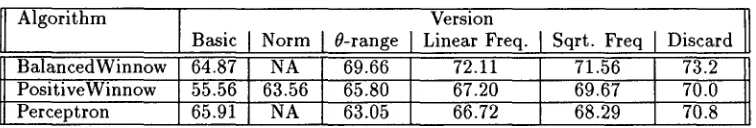
We started by evaluating the basic versions of the three algorithms. T h e features we use throughout the experiments are single words, at the lemma level, for nouns and verbs only, with minimal frequency of 3 occurrences in the corpus. In the basic versions the strength of the feature is taken to indicate only the presence or absence of f in the document, that is, it is either 1 or 0. T h e training algorithm was run iteratively on the training set, until no mistakes were made on the training collection or until some upper bound (50) on the number of iterations was reached. The results for the basic versions are shown in the first column of Table 1.

4 E x t e n s i o n s t o t h e B a s i c a l g o r i t h m s 4.1 L e n g t h V a r i a t i o n a n d N e g a t i v e features Text documents vary widely in their length and a text classifier needs to tolerate this variation. This issue is a potential problem for a linear classifier which scores a document by summing the weights of all its active features: a long document may have a better chance of exceeding the threshold merely by its length.

This problem has been identified earlier on and attracted a lot of work in the classical work on IR (Salton and Buckley, 1983), as we have indicated in Section 2.2. T h e treatment described there ad- dresses at the same time at least two different con- cerns: length variation of documents and feature repetition. In this section we consider the first of those, and discuss how it applies to the algorithms we investigate. T h e second concern is discussed in Section 4.3.

Algorithms that allow the use of negative features, such as BalancedWinnow and Perceptron, tolerate variation in the documents length naturally, and thus have a significant advantage in this respect. In these cases, it can be expected that the cumulative contribution of the weights and, in particular, those that are not indicative to the current category, does not count towards exceeding the threshold, but rather averages out to 0. Indeed, as we found out, no special normalization is required when using these algorithms. Their significant advantage over the unnormalized version of PositiveWinnow is readily seen in Table 1.

(6)

Algorithm Version Basic Norm 0-range Linear Freq.

BalancedWinnow 64.87 NA 69.66 72.11

PositiveWinnow 55.56 63.56 65.80 67.20

Perceptron 65.91 NA 63.05 66.72

Sqrt. Freq Discard

71.56 73.2

69.67 70.0

68.29 70.8

Table 1: Recall/precision break-even point (in percentages) for different versions of the algorithm. Each figure is an average result for two pairs of training and testing sets, each containing 2000 training documents and 1000 test documents.

only rarely occurs in text categorization and thus the main use of the negative features is to tolerate the length variation of the documents.

When using PositiveWinnow, which uses only positive weights, we no longer have this advantage and we seek a modification that tolerates the variation in length. As in the standard IR solution, we suggest to modify

s(f, d),

the strength of the feature f in d, by using a quantity that is normalized with respect to the document size.

Formally, we replace the strength

s(f,d)

(which may be determined in several ways according to feature frequency, as explained below) by a

normalized

strenglh,

s(f, d)

sn(f, d)

= E fEd

s(f, d)"

In this case (which applies, as discussed above, only for PositiveWinnow), we also change the initial weight vector and initialize all the weights to 0.

Using normalization gives an effect that is similar to the use of negative weights, but to a lesser degree. The reason is that it is used uniformly; in long documents, the number of indicative features does not increase significantly, but their strength, neverthe- less, is reduced proportionally to the total number of features in the document. In the long version of the paper we present a more thorough analysis of this issue.

T h e results presented in Table 1 (second column) show the significant improvements achieved in Pos- itiveWinnow performance, when normalization is used. In all the results presented from this point on, positive winnow is normalized.

4.2 U s i n g T h r e s h o l d r a n g e

Training a linear text classifier is a search for a weight vector in the feature space. The search is for a linear separator that best separates documents t h a t are relevant to the category from those that are not. In general, there is no guarantee that a weight vector of this sort exists, even in the training data, but a good selection of features make this more likely. While the basic versions of our algorithms search for linear separators, we have modified those so that our search for a linear classifier is biased to look for "thick" classifiers. To understand this, consider, for

the moment, the case in which all the data is per- fectly linearly separable. Then there will generally be many linear classifiers that separate the training d a t a we actually see. A m o n g these, it seems plausible that we have a better chance of doing well on the unseen test data if we choose a linear separator that separates the positive and negative training examples as "widely" as possible. T h e idea of having a wide separation is less clear when there is no perfect separator, but we can still appeal to the basic intuition.

Using a "thick" separator is even more important when documents are ranked rather than sim- ply classified; that is, when the actual score produced by the classifier is used in the decision process. T h e reason is that if

Fc(d)

is the score produced by the classifier

Fc

when evaluated on the document d then, under some assumptions on the dependencies among the features, the probability that the document d is relevant to the category c is given by

Prob(d E c) _ l+e=~;r~7

This function, known as the

sigmoid

function, "flattens" the decision region in a way that only scores that are far apart from the threshold value indicate t h a t the decision is made with significant probability.

Formally, among those weight vectors we would like to choose the hyper-plane with the largest "separating parameter", where the separating parameter r is defined as the largest value for which there exists a classifier F¢ (defined by a weight vector w) such that for all positive examples

d, F¢(d) > 0 + r/2

and for all negative d,

Fc(d) < 0 - r/2.

[image:6.612.125.503.69.133.2]

(7)

The results presented in the third column of Ta- ble 1 show the improvements obtained when the threshold range is used. In all the results presented from this point on, all the algorithms use the threshold range modification.

4.3 F e a t u r e R e p e t i t i o n

Due to the bursty nature of term occurrence in documents, as well as the variation in document length, a feature may occur in a document more than once. It is therefore important to consider the frequency of a feature when determining its strength. On one hand, there are cases where a feature is more indicative to the relevance of the document to a category when it appears several times in a document. On the other hand, in any long document, there may be some random feature that is not significantly indicative to the current category although it repeats many times. While the weight of f in the weight vector of the category,

w(f,

c), may be fairly small, its cumulative contribution might be too large if we increase its strength,

s(f, d),

in proportion to its frequency in the document.

As mentioned in Section 2.2, the classical IR literature has addressed this problem using the i f and

idf

factors. We note that the standard treatment in IR suggests a solution to this problem that suits batch algorithms - algorithms that determine the weight of a feature after seeing all the examples. We, on the other hand, seek a solution that can be used in an on-line algorithm. Thus, the frequency of a feature throughout the data set, for example, cannot be taken into account and we take into account only the if term. We have experimented with three alterna- tive ways of adjusting the value of

s(f, d)

according to the frequency of the feature in the document: (1) Our default is to let the strength indicate only the activity of the feature. T h a t is,

s(f, d) =

1, if the feature is present in the document (active feature) and

s(f,

d) = 0 otherwise. (2)

s(f,d) = n(f,d),

where

n(f, d)

is the number of occurrences of f in d; and (3)

s(f, d) = ~

d)

(as in (Wiener, Pedersen, and Weigend, 1995)). These three alternatives examine the tradeoff between the positive and negative im- pacts of assigning a strength in proportion to feature frequency. In most of our experiments, on different data sets, the choice of using

~/n(f, d)

performed best. The results of the comparative evaluation appear in columns 3, 4, and 5 of Table 1, corresponding to the three alternatives above.

4.4 D i s c a r d i n g f e a t u r e s

Multiplicative update algorithm are known to tolerate a very large number of features. However, it seems plausible that most categories depend only on fairly small subsets of indicative features and not on all the features that occur in documents that belong to this class. Efficiency reasons, as well as the occa- sional need to generate comprehensible explanations

to the classifications, suggest t h a t discarding irrelevant features is a desirable goal in IR applications. If done correctly, discarding irrelevant features may also improve the accuracy of the classifier, since irrelevant features contribute noise to the classification score.

An important property of the algorithms investi- gated here is that they do not require a feature selection pre-processing stage. Instead, they can run in the presence of a large number of features, and allow for discarding features "on the fly", based on their contribution to an accurate classification. This property is especially i m p o r t a n t if one is considering enriching the set of features, as is done in (Golding and Roth, 1996; Cohen and Singer, 1996); in these cases it is important to allow the algorithm to decide for itself which of the features contribute to the accuracy of the classification.

We filter features that are irrelevant for the category based on the weights they were assigned in the first few training rounds.

The algorithm is given as input a range of weight value which we call the

filtering range.

First, the training algorithm is run for several iterations, until the number of mistakes on the training data drops below a certain threshold. After this initial training, we filter out all the features whose weight lie in this filtering range. Training then continues as usual.

There are various ways to determine the filtering range. T h e obvious one may be to filter out all features whose weight is very close to 0, but there are a few subtle issues involved due to the normalization done in the PositiveWinnow algorithm. In the results presented here we have used, instead, a different filtering range: Our filtering range is centered around the initial value assigned to the weights (as specified earlier for each algorithm), and is bounded above and below by the values obtained after one promotion or demotion step relative to the initial value. Thus, with high likelihood, we discard features which have not contributed to many mistakes - those that were promoted or demoted at most once (possibly, with additional promotions and demotions which canceled each other, though).

T h e results of classification with feature filtering appear in the last column of Table 1. We hypothe- size that the improved results are due to reduction in the noise introduced by irrelevant features. Fur- ther investigation of this issue will be presented in the long version of this paper. Typically, about two thirds of the features were filtered for each category, significantly reducing the o u t p u t representation size.

(8)

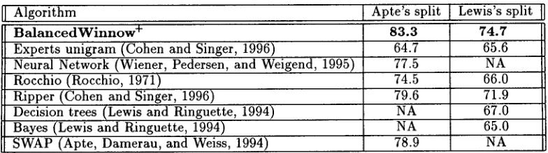
Algorithm

B a l a n c e d W i n n o w +

Experts unigram (Cohen and Singer, 1996)

Neural Network (Wiener, Pedersen, and Weigend, 1995) Rocchio (Rocchio, 1971)

Ripper (Cohen and Singer, 1996)

Decision trees (Lewis and Ringuette, 1994) Bayes (Lewis and Ringuette, 1994)

SWAP (Apte, Damerau, and Weiss, 1994)

Apte's split 8 3 . 3

64.7

Lewis's split 74.7

65.6

77.5 NA

74.5 66.0

79.6 71.9

NA 67.0

NA 78.9

65.0 NA

Table 2: Break-even points comparison. The data is split into training set and test set based on Lewis's split - (Lewis, 1992), 14704 documents for training, 6746 for testing, and Apte's split - (Apte, Damerau, and Weiss, 1994), 10645 training, 3672 testing, omitting documents with no topical category.

now algorithm, which incorporates the 0-range modification, a square-root of occurrences as the feature strength and the discard features modification (BalancedWinnow + in Table 2).

We have compared this version with a few other algorithms which have appeared in the literature on the complete Reuters corpus. Table 2 presents break-even points for BalancedWinnow + and the other algorithms, as defined in Section 2.3.

The results are reported for two splits of the complete Reuters corpus as explained in Section 2.3. The algorithm was run with iterations, threshold range, feature filtering, and frequency-square-root feature strength.

The first two rows in Table 2 compare the performance of BalancedWinnow + with the two algorithms that most resemble our approach, the Ex- perts algorithm from (Cohen and Singer, 1996) and a neural network approach presented in (Wiener, Ped- ersen, and Weigend, 1995). (see Section 2.2).

Rocchio's algorithm is one of the classical algorithms for this tasks, and it still performs very good compared to newly developed techniques (e.g, (Lewis et al., 1996)). We also compared with the Ripper algorithm presented in(Cohen and Singer, 1996) (we present the best results for this task, with negative tests), a simple decision tree learning system and a Bayesian classifier. The last two figure are taken from (Lewis and Ringuette, 1994) where they were evaluated only on Lewis's split. The last comparison is with the learning system used by (Apte, Damerau, and Weiss, 1994), SWAP, which was evaluated only on Apte's split.

Our results significantly outperform (by at least 2- 4%) all results which appear in t h a t table and use the same set of features (based on single words). Of the results we know of in the literature, only a version of the Experts algorithm of (Cohen and Singer, 1996) which uses a richer feature set - sparse word trigrams - outperforms our result on the Lewis split, with a break-even point of 75.3%, compared with 74.6% for the unigram-based BalancedWinnow + . However,

this version achieves only 75.9% on the Apte split (compared with 83.3% of BalancedWinnow+). In the long version of this paper we plan to present the results of our algorithm on a richer feature set as well.

6 C o n c l u s i o n s

Theoretical analyses of the Winnow family of algorithms have predicted an exceptional ability to deal with large numbers of features and to adapt to new trends not seen during training. Until recently, these properties have remained largely undemonstrated.

We have shown that while these algorithms have m a n y advantages there is still a lot of room to explore when applying them to a real-world problem. In particular, we have demonstrated (1) how variation in document length can be tolerated through either normalization or negative weights, (2) the positive effect of applying a threshold range in training, (3) alternatives in considering feature frequency, and (4) the benefits of discarding irrelevant features as part of the training algorithm. The main contribution of this work, however, is that we have presented an algorithm, BalancedWinnow +, which performs significantly better than any other algorithm tested on these tasks using unigram features.

[image:8.612.117.509.69.179.2]

(9)

n e e d e d on policies o f d i s c a r d i n g f e a t u r e s a n d a v o i d - ance o f o v e r - f i t t i n g . In c o n c l u s i o n , we suggest t h a t t h e d e m o n s t r a t e d a d v a n t a g e s o f t h e W i n n o w - f a m i l y o f a l g o r i t h m s m a k e it a n a p p e a l i n g c a n d i d a t e for fur- t h e r use in t h i s d o m a i n .

A c k n o w l e d g m e n t s

T h a n k t o M i c h a l L a n d a u for her h e l p in r u n n i n g t h e e x p e r i m e n t s .

R e f e r e n c e s

Apte, C., F. Damerau, and S. Weiss. 1994. Towards language independent automated learning of text categorization models. In Proceedings of ACM-SIGIR Con- ference on Information Retrieval.

Blum, A. 1992. Learning boolean functions in an infi- nite a t t r i b u t e space. Machine Learning, 9(4):373-386, October.

Blum, A. 1995. Empirical support for Winnow and weighted-majority based algorithms: results on a cal- endar scheduling domain. In Proc. 12th International Conference on Machine Learning, pages 64-72. Mor- gan Kaufmann.

Cesa-Bianchi, N., Y. Freund, D. P. Helmbold, D. Haus- sler, and R. E. Schapire a n d M. K. Warmuth. 1995. How to use expert advice, pages 382-391.

Cesa-Bianchi, N., Y. Freund, D. P. Helmbold, and M. Warmuth. 1994. On-line prediction and conver- sion strategies. In Computational Learning Theory: Eurocolt '93, volume New Series Number 53 of The Institute of Mathematics arid its Applications Confer- ence Series, pages 205-216, Oxford. Oxford University Press.

Cohen, W. W. and Y. Singer. 1996. Context-sensitive learning methods for text categorization. In Proc. of the 19th Annual Int. ACM Conference on Research and Development in Information Retrieval.

Cortes, Corinna and Vladimir Vapnik. 1995. Support- vector networks. Machine Learning, 20(3):273-297.

Duda, R. O. and P. E. Hart. 1973. Pattern Classification and Scene Analysis. Wiley.

Golding, A. R. and D. Roth. 1996. Applying winnow to context-sensitive spelling correction. In Proc. of the International Conference on Machine Learning.

Herbster, M. a n d M. Warmuth. 1995. Tracking the best expert. In Proc. 12th International Conference on Machine Learning, pages 286-294. Morgan Kanf- mann.

Kivinen, J. and M. K. Warmuth. 1995a. Exponentiated gradient versus gradient descent for linear predictors. In Proc. of STOC. Tech Report UCSC-CRL-94-16.

Kivinen, J. and M. K. Warmuth. 1995b. The perceptron algorithm vs. Winnow: linear vs. logarithmic mistake bounds when few input variables are relevant. In Proc. 8th Annu. Conf. on Comput. Learning Theory, pages 289-296. ACM Press, New York, NY.

Lewis, D. 1992. An evaluation of phrasal and clustered representations on a text categorization problem. In

Proc. of the 15th Int. ACM-SIGIR Conference on In- formation Retrieval.

Lewis, D. and M. Ringuette. 1994. A comparison of two learning algorithms for text categorization. In Proc. of Symposium on Document Analysis and Information Retrieval.

Lewis, D., R. E. Schapire, J. P. Callan, and R. Papka. 1996. Training algorithms for linear text classifiers. In SIGIR '96: Proc. of the 19th Int. Conference on Research and Development in Information Retrieval, 1996.

Littlestone, N. 1988. Learning quickly when irrelevant a t t r i b u t e s abound: A new finear-threshold algorithm.

Machine Learning, 2:285-318.

Littlestone, N. 1991. Redundant noisy attributes, attribute errors, and linear threshold learning using Winnow. In Proc. $th Annu. Workshop on Corn- put. Learning Theory, pages 147-156, San Mateo, CA. Morgan Kanfmann.

Littlestone, N. 1995. Comparing severallinear-threshold learning algorithms on tasks involving superfluous attributes. In Proc. 12th International Conference on Machine Learning, pages 353-361. Morgan Kauf-

m a n n .

Littlestone, N. and M. K. Warmuth. 1994. The weighted m a j o r i t y algorithm. Information and Computation,

108(2):212-261.

Rocchio, 3. 1971. Relevance feedback information retrieval. In G. Salton, editor, The S M A R T retrieval system - experiments in automatic document process- ing. Prentice-Hall, pages 313-323.

Rosenblatt, F. 1958. The perceptron: A probabilistic model for information storage and organization in the brain. Psychological Review, 65:386-407. (Reprinted in Neurocomputing (MIT Press, 1988).).

Salton, G. and C. Buckley. 1983. Introduction to Modern Information Retrieval. McGraw-Hill.

Tzeras, K. and S. Hartmann. 1993. A u t o m a t i c index- ing based on bayesian inference networks. In Proc. of 16th Int. ACM SIGIR Conference on Research and Development in Information Retrieval.